Dead Reckoning for Trajectory Estimation of Underwater Drifters under Water Currents - MDPI
←
→
Page content transcription
If your browser does not render page correctly, please read the page content below
Journal of
           Marine Science
           and Engineering

Article
Dead Reckoning for Trajectory Estimation of
Underwater Drifters under Water Currents †
Itzik Klein ∗,‡      and Roee Diamant ‡
 Department of Marine Technologies, University of Haifa, Haifa 3498838, Israel; roee.d@univ.haifa.ac.il
 * Correspondence: kitzik@univ.haifa.ac.il
 † This work was partly funded by the MOST-BMBF German-Israeli Cooperation in Marine Sciences 2018–2020.
 ‡ These authors contributed equally to this work.

 Received: 21 January 2020; Accepted: 13 March 2020; Published: 16 March 2020

 Abstract: Between external position updates, the most useful technique for trajectory estimation of
 a submerged drifter is dead reckoning (DR). These devices drift with the water current to measure
 the current’s velocity or to observe physical phenomena. We focus on the specific but important case
 of when the drifter, due to its size and shape, experiences acceleration by the water current, an effect
 that must be taken into account during the DR. The force induced by the water current over the
 drifter is translated into a shift in the heading direction, thus creating a horizontal (sideslip) and
 a vertical (angle of attack) directional angles between the drifter’s moving direction and its body
 frame. In this paper, we extend and modify techniques used for pedestrian DR and propose PCA-DR:
 a principle component analysis-based DR algorithm to estimate the directional angles. Used for cases
 where the water current is significant such that its force induces acceleration over the drifter and used
 only for short time periods of a few seconds between navigation fixes, PCA-DR uses acceleration
 measurements only and does not assume knowledge of the drifter’s dynamics. Instead, as part of the
 DR process, PCA-DR estimates the directional angles induced by the water current. Compared to the
 traditional DR approach, our results demonstrate good navigation performance. A designated sea
 experiment demonstrates the applicability of PCA-DR in a realistic sea environment.

 Keywords: principal component analysis (PCA); underwater navigation; subsea drifter; dead reckoning;
 sideslip angle; angle of attack

1. Introduction
      Subsea drifters (drift with the water current) are used for a variety of applications, including the
gathering of scientific data and climate monitoring, to name a few [1,2]. In all applications, the device
has no positioning aided solutions while being submerged, so the navigation system is critical, enabling
the user to infer the drifter’s measurements with its geographic location. The role of the navigation
system is to determine the position, velocity, and attitude of the device while being submerged
and while drifting or maneuvering. We consider freely drifting devices that are not connected to,
e.g., a surface buoy. Due to the water conductivity, GPS signals are not received by these drifters,
so GPS positioning is not available. In such situations, the main underwater navigation techniques fall
into one of the following three categories [3]:

1.    Inertial Navigation Systems (INSs): An INS uses accelerometers and gyroscopes and requires
      initial conditions to calculate the device state through dead reckoning (DR). Although the full state
      can be determined by the INS, it suffers from an inherent drift. This is because the INS-measured
      quantities contain noises and biases that are integrated to obtain the device state [4]. Therefore,
      INSs are usually fused with external sensors [5] or information about the environment [6,7] to
      compensate for this drift.

J. Mar. Sci. Eng. 2020, 8, 205; doi:10.3390/jmse8030205                         www.mdpi.com/journal/jmse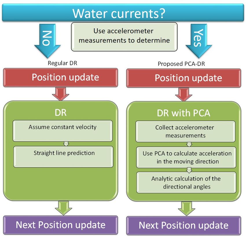
J. Mar. Sci. Eng. 2020, 8, 205                                                                               2 of 22

2.     Acoustic Localization: Acoustic localization provides the navigation system with position fixes
       by measuring the device’s range to nodes of known positions, referred to as anchors. Acoustic
       ranging is based on measuring the time-of-flight (TOF), the time-difference-of-flight (TDOF),
       or the signal strength of an acoustic signal from the anchor to the submerged device. Ranging
       can be carried out passively or actively, but in either case requires the existence of at least one
       anchor in the acoustic range [8,9].
3.     Geophysical Navigation: In geophysical navigation, features from the environment are used as
       navigation reference points, usually employing cameras [10] or different types of sonar [11] for
       terrain-based tracking [12] or simultaneous localization and mapping [13].

      In addition, underwater navigation is often performed by means of sensor fusion. For example,
frameworks for the navigation of autonomous underwater vehicles (AUVs) based on, e.g., an extended
Kalman filter or an Unscented Kalman filter combine data from inertial measurements, acoustic
beacons, Doppler velocity loggers, and others, and obtain high performance. Yet, multimodal
navigation aid sensors are often scarce in low-cost systems such as drifters. Out of the three categories,
the INS is the most popular since it does not require specific knowledge of the environment or
uses external sources of information. Consequently, the context of this work is a DR navigation of
a subsea drifter using only the device’s self-measured accelerometers. In this context, a DR approach
for the self-navigation of submerged drifting nodes is a cost-effective solution with several advantages.
First, it is a standalone system that uses only an inertial navigation unit and does not require any
information/transmissions from external sources. Second, different from filtering techniques, DR does
not require information about the mobility pattern of the tracked device or on the hydrodynamics of the
device. As such, DR is a cost-effective robust navigation solution that best fits low-cost systems such
as submerged drifters. Moreover, DR navigation is needed for short time periods between external
position updates such as long baseline systems (LBLs) or from global navigation satellite systems
(GNSSs). Trajectory estimation using DR does not require the modeling of the drifter’s dynamics,
nor does it require a prior assumption about the motion type of the drifter. Instead, it updates the
dynamic state on the fly based on the INS measurements.

1.1. Scope of Work
     DR assumes that the underwater platform nominally follows a dynamic model between two
successive position updates; yet, as a result of water currents, in practice, the device is subject to
an unknown moving direction, whose estimation is crucial to the success of the DR process. Since the
drifter’s motion is affected only by the motion of the water current, which, due to the non-negligible
size and shape of the drifter, is an acceleration-driving force [14], this uncertainty in the moving
direction occurs when the induced force operates at certain horizontal and vertical angles with respect
to the body frame of the drifter. As illustrated in Figure 1a,b, the angles considered are γh and γv .
We refer to these angles as the directional angles, and consider the case where directional angles are
formed by the water current.

                                       (a)                                  (b)

      Figure 1. Illustration of the acceleration triangle experienced by a subsea device. The force induced
      by the water current over the drifter is translated into a shift in the heading direction, thus creating
      an horizontal and/or vertical directional angles between the drifter’s moving direction and its body
      frame. (a) Horizontal plane; (b) vertical plane.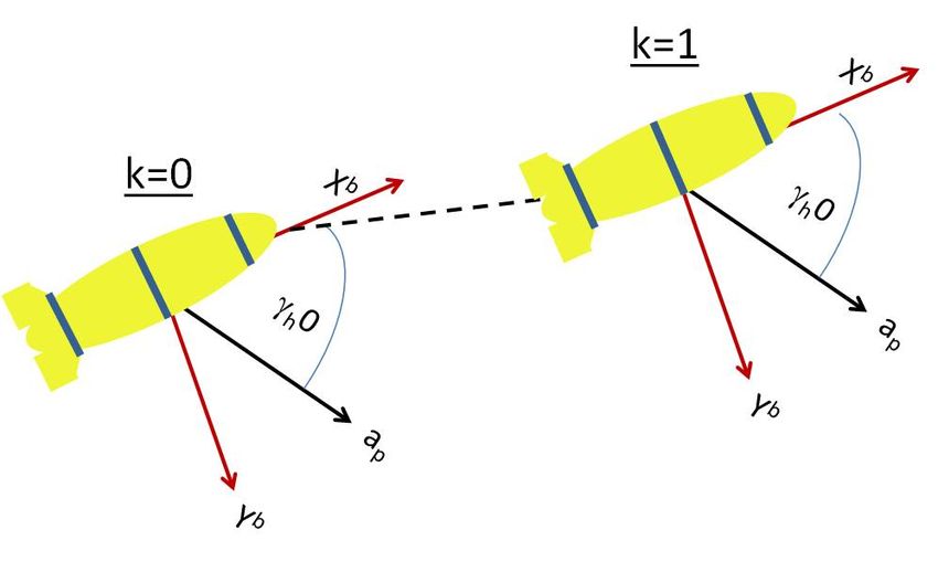
J. Mar. Sci. Eng. 2020, 8, 205                                                                                   3 of 22

     Performing DR directly on the acceleration measurements without compensating for the
directional angles would result in large errors. This is evident by the velocity triangle illustrated
in Figure 2a,b. In the horizontal plane, the directional angles result in a sideslip angle, denoted by β in
Figure 2a, which is the angle between the drifter’s horizontal velocity with respect to the water and its
horizontal velocity in the body frame. In the vertical plane, the directional angles render an angle of
attack, denoted by α in Figure 2b, which is the angle between the drifter’s vertical velocity with respect
to the water and its vertical velocity in the body frame. The result of the existence of both a sideslip
angle and an angle of attack is a shift in the drifter’s moving direction, which must be compensated
for in the DR process. More specifically, since both the horizontal and vertical directional angles
affect the acceleration measurements that are measured in the body frame, without estimating the
current’s acceleration, a p , or the values of γh and γv from Figure 1a,b, respectively, DR is not possible.
To further support this claim, in Figure 3, we show the results of the DR position error as a function
of the directional angle on the horizontal plane, γh , when this angle is not compensated (results are
obtained using the simulation setup reported in Section 5). As expected, the results show that DR
performance greatly deteriorates with the increase of γh . Besides the need to estimate the directional
angles for DR navigation, evaluating their value has the practical implementation of path planning in
case the drifter can control its depth (e.g., [2]).

                                 (a)                                                 (b)

          Figure 2. Illustration of the projected velocity triangle. (a) Horizontal plane; (b) vertical plane.

      Figure 3. Dead reckoning (DR) position error when the horizontal directional angle is not compensated.

     The effect of the directional angles on the drifter’s motion is very similar to the effect an aircraft
experiences, due to the wind factor. However, unlike in aircrafts, where the wind speed and direction
can be measured directly using the pitot tube [15], direct measurement of the water current is
challenging and is generally performed by maneuvering. This, of course, is not possible in the
case of drifters. Traditionally, the sideslip angle can be estimated by gyroscopes, by magnetometers,
J. Mar. Sci. Eng. 2020, 8, 205                                                                      4 of 22

or by GNSSs, as will be elaborated in Section 2.2. Yet, while the drifter is submerged, the GNSS is
not available, and the magnetometer measurements are subject to varying interferences from the
surrounding environment. Additionally, high precision gyroscopes are very expensive, and simple
submerged floaters use low grade gyroscopes whose noise cannot be filtered easily, due to the rapidly
changing marine environment that include thermoclines and turbulances. As a result, it is challenging
to accurately measure the directional angles. Considering the problem of obtaining cost-effective
gyroscopes and magnetometers, we propose a method that estimates the directional angles between
two successive position updates based only on acceleration measurements and performs DR based on
this type of estimation. Our method becomes effective for drifters with low-to-moderate gyroscope
sensors in the common scenario when the device’s motion is set by the water currents. Our work is
limited to the cases where an acceleration force operates on submerged drifters, such that DR can
be performed.

1.2. Contribution
      Our contribution is in the trajectory estimate for submerged drifters between two known locations,
while taking into account the effect of the water current on the drifter’s velocity. Due to the limitation
of the acceleration-only DR approach, the time period considered for performing the DR is on the order
of a few seconds. This is applicable in cases where periodic location fixes are received. For example,
the work in [2] presents an application for a flock of submerged drifters aiming to estimate ocean
currents and to track migration patterns of biofauna. These drifters include an acoustic recorder to
receive signals from a set of on-surface anchored acoustic beacons. These beacons generate periodic
acoustic emissions every few seconds such that, using long baseline acoustic positioning, the drifters
can be localized offline. Between such acoustic-based fixes, there is a need to estimate the trajectory of
the drifters.
      Our approach does not require the estimation or prediction of the water current, nor does it
need the information of the drifter’s dimensions, thereby achieving robustness to the shape of the
drifter in use and to the sea conditions. We offer this capability based on low-cost accelerometers only,
which is important since long deployment drifters do not allow for the insertion of energy-hungry and
expensive instruments such as acoustic Doppler current profiling (ADCP). Consequently, when the
water current is substantial, to the best of our knowledge, ours is the only approach that allows subsea
positioning for drifters.
      Our method, referred to as PCA-DR, makes use of the principle component analysis (PCA)
method to estimate the moving direction of the drifter. Once the moving direction is determined,
we derive the DR algorithm and its closed form expressions to evaluate its performance as a function
of the involved parameters. PCA-DR is inspired by the successful application of DR-based pedestrian
navigation in [16], where PCA is used to estimate the walking direction regardless of the smartphone
direction. Yet, while most of the time a pedestrian is moving horizontally and thus only the horizontal
angle needs to be determined, an underwater platform can also move in a vertical direction. Hence,
the vertical directional angle should also be considered to determine the moving direction. Moreover,
while pedestrian navigation can be aided by reference points at times when the foot touches the ground
and the velocity is zero, the motion of a submerged floater is continuous. Considering these challenges,
we derive a modification to the PCA approach, which enables the estimation of the angles affecting the
submerged device’s moving direction based on accelerometer readings. When the platform applies
no acceleration but undergoes accelerations due to water currents, the proposed approach can also
estimate the angles between the moving direction of the platform and its x-axis in the body frame.
Like all DR approaches, PCA-DR is limited to short time intervals, usually on the order of a few seconds,
before the navigation solution drifts. However, different from common DR, PCA-DR also provides
a navigation solution in the presence of a water current’s force. This also means that PCA-DR is
applicable only in the presence of an observable acceleration-induced force over the submerged drifter.
J. Mar. Sci. Eng. 2020, 8, 205                                                                        5 of 22

     While both DR and PCA are well explored techniques, ours is the first method to combine the
two for the task of location-tracking drifters in the presence of a water current. For drifters, the effect
of the water current has not been explored, although, as we show in our analysis, navigation fails if
this effect is neglected. Moreover, while previous approaches have used PCA and DR sequentially,
ours is the first work to use PCA as part of the DR process. The result is an iterative estimation of
water-current-induced directional angles. This task is performed using only acceleration measurements.
This is mostly appealing for drifters whose cost and energy limitations are substantial and thus cannot
support maneuvering or Doppler shift measurements.
     Our list of contributions is threefold:

•      a compensation for the directional angles when DR navigation is required;
•      the estimation of directional angles using acceleration measurements only for short time periods
       of a few seconds between two successive position updates;
•      a simplified DR approach for submerged floaters under the effect of directional angles for
       online/offline trajectory estimation.

     We evaluate the performance of the proposed approach in the presence of a water current in both
numerical and experimental investigations including a drifting buoy with a self-made INS. The results
show a great improvement over benchmark DR solutions.
     The remainder of this paper is organized as follows: In Section 2, we describe current approaches
for sideslip angle estimation and for transformation, to coordinate between the navigation frames
used in the paper. In Section 3, our proposed approach for estimating directional angles is described,
and in Section 4 the DR algorithm and its derivations are presented. Section 5 shows the analysis and
numerical and experimental results. Conclusions are presented in Section 6.

2. Preliminaries
      Different from filtering-based navigation techniques that require modeling of the dynamics of the
submerged platform, DR does not follow a specific model. As a result, DR is robust to the navigating
platform and does not require knowledge of its hydro-dynamic profile. For this reason, DR is accepted
as the most practical solution for subsea navigation. In basic terms, DR is the process whereby the
current position of a tracked platform is calculated based on its last known position. With no dynamic
model to follow, the tracking is based on measurements of speed and direction. One of the most
common implementations of DR is inertial navigation. Here, inertial sensors (accelerometers and
gyroscopes) provide measurements of rotational and translational motion of the tracked platform,
and additional information in the form of external sensors or movement type can be added (see our
analysis in [17]). Our PCA-DR is a DR process that takes into account the effect of the water current.
In PCA-DR, we consider DR between two successive position measurements using only accelerometers.
      In the following, we describe current works for pedestrian navigation using the PCA method,
and briefly review two related subjects used in the derivation of the methodology presented herein:
(1) the transformation of coordinate frames, and (2) principle component analysis. We then present our
system’s model.

2.1. Approaches for Underwater Dead Reckoning
     While the challenge of geo-locating a drifter is not fully addressed, a large body of literature offers
solutions for the location tracking of autonomous underwater vehicles (AUVs). In [18], a few filtering
approaches are compared for the location estimate of an AUV. The methods assume a motion model
whose parameters are updated by filtering techniques, and the work in [19] uses the motion model
to identify faulty sensory information. Considering the challenge in determining a motion model,
the methods in [20,21] use unconventional filtering techniques with the aim of being robust to various
dynamics and noise distribution types. Instead, the works in [22–24] use the known dimensions of the
AUV to form a hydrodynamic model, which, in turn is used in the filtering scheme to obtain a better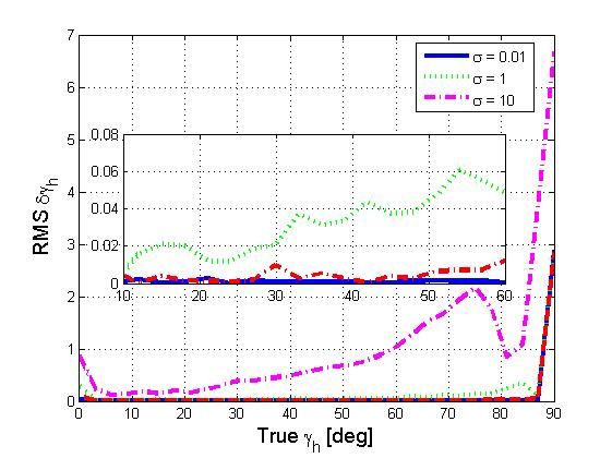
J. Mar. Sci. Eng. 2020, 8, 205                                                                      6 of 22

dynamic model. Results from sea experiments show good performance. However, we suspect these
are performed in low water currents, as almost no consideration is given to the water current that
introduces an external force, and can significantly affect small devices such as drifters.
     While in PCA-DR we do not assume knowledge of the water current, some approaches have
been suggested to compensate for a given or directly measured water current. The work in [25] takes
into account the water current along the water column during the DR operation. The solution offered
directly measures the water current using a Doppler velocity logger or an acoustic Doppler current
profiler positioned on an AUV, and integrates this data in the filtering scheme. However, such systems
are energy- and cost-expensive and may not fit the case of low-cost drifters such as Argo floats, cf. [1].
External forces are also considered in [26], where a full-scaled inertial measurement unit is employed
to combine acceleration measurements, gyrocompasses, and magnetometers in a filtering scheme.
Experiments show results when an external magnetic force is present. Yet, here too, a motion model is
employed, and directional angles induced by the water current are ignored. The need for data about
the water current is acknowledged in [27], where a group of AUVs cooperates by sharing information
about mismatches found from a water current forecast. Similarly, in [28], we tracked the location
of a submerged node also using drifting information from nearby beacons. However, the success
of these approaches largely depends on the spatial stability of the water current, and requires prior
knowledge of the environment, e.g., bathymetry, temperature, and tied fluctuations, which are often
hard to obtain.

2.2. Common Approaches for Sideslip Angle Estimation
     For land vehicles, the sideslip angle must be evaluated to guarantee the vehicle’s stability.
Considering the problematic fact that the drifter’s sideslip angle cannot be measured directly, several
approaches have been suggested to estimate the sideslip angle [29] or, equivalently, to evaluate
the lateral velocity [30,31]. These approaches rely on modeling the device’s dynamics, and require
measurements from sensors such as gyroscopes, accelerometers, magnetometers and GPS. Similar to
underwater navigation, in the pedestrian navigation context, obtaining such measurements requires
high-precision and expensive sensors. Therefore, different approaches have been suggested for the
same problem of estimating the walking direction.
     We find that the most promising methods for estimating directional angles are the PCA
method [16,32], Forward and Lateral Accelerations modeling (FLAM) [33], and the Frequency analysis
of Inertial Signals (FIS), as indicated in [34]. The PCA approach is further elaborated in Section 2.4;
however, we emphasize here that the PCA approach requires only accelerometer data and thus is
most suitable for underwater navigation, which bears a low cost and is short on energy and on
accurate sensors. In FLAM, the approach models the forward and lateral accelerations by the sum of
sinusoids. The angle pointing towards the heading direction is found to be the one that maximizes
the correlation of the estimated acceleration and the pre-determined model. As in the PCA approach,
only accelerometer data are required from the sensors, but, in addition, walking pattern modeling is
also needed. This may result in model mismatch for underwater maneuvering, which is affected by
non-linear complex phenomena such as water currents, turbulence, and sea waves. In the FIS approach,
both accelerometer and gyroscope outputs are used. The main idea is to find the direction that
maximizes the spectral density of the accelerometer and gyroscope signals’ energy for the step/stride
frequency [35,36].
     The sideslip angle estimation for underwater navigation is thus far handled in the context
of path-following controller design [37]. In this case, the sideslip angle is treated as an unknown,
small, and constant parameter during straight line paths. The switching between the segments appears
as steps in the parameter update law. For vehicles traversing a non-circular path, the method utilizes
the fact that the sideslip angle varies much more slowly than the control bandwidth to estimate the
varying sideslip using a nonlinear adaptation law. Other works use a zero sideslip angle assumption
supported by sea experiments to carry out controller design analysis [38] or parameter identification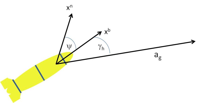
J. Mar. Sci. Eng. 2020, 8, 205 7 of 22
for a nonlinear simulation [39]. However, as we show in our analysis, neglecting the sideslip and the
directional angles may result in large navigation errors.
2.3. Coordinate Frames and Transformations
To manage directional angle estimations, we need to coordinate the body reference frame (b-frame)
with the stability frame (s-frame) and the current reference frame (c-frame). While the acceleration
measurements are given in the b-frame, for navigation purposes they should be translated onto the
s-frame. This transformation should take into account the effect of the water current, which resides in
the c-frame. Referring to Figure 2a,b, the b-frame is the drifter’s fixed coordinate system. The origin
of the coordinates is located at a convenient position in relation to the device, usually the center of
buoyancy. The x b axis points towards the front of the drifter, the yb axis points towards the right
of the drifter (starboard), and the zb axis completes the right-handed orthogonal frame pointing to
the bottom (the keel). The s-frame is fixed to the drifter at the same origin as the b-frame. The x s
axis points along the speed vector projection onto the x b -zb plane, the ys axis coincides with the yb
axis, and the zs axis completes the right-handed coordinate system. The c-frame, like the b-frame and
s-frame, has its origin fixed. The x c axis is aligned with the current’s speed vector, zc coincides with zs ,
and yc completes the right-handed coordinate system.
To transfer between these three coordinate frames, we use two angles: the angle of attack, denoted
by α, and the sideslip angle, denoted by β. The angle of attack is shown in the vertical plane (Figure 2b),
together with the pitch angle θ. The sideslip angle is shown in the horizontal plane (Figure 2a) with
the heading angle, ψ. The angle of attack is defined as being positive for a right-handed rotation from
the stability frame’s x s axis to the body frame’s x b axis. Hence, a left-handed rotation is needed for the
transformation between the b- and s-frames such that
cos(α) 0 sin(α)
Tbs (α) = 0 1 0 . (1)
− sin(α) 0 cos(α)
The sideslip angle is the angle between the water current speed vector and the x b -zb plane. The
sideslip is used to define the transformation between the s- and w-frames through
cos( β) sin( β) 0
s,c
T ( β) = − sin( β) cos( β) 0 . (2)
0 0 1
Finally, the transformation between the b-frame and the c-frame is obtained by multiplying matrix
Tbs from Equation (1) with matrix T s,c from Equation (2). Denoting cos(α) = cα , sin(α) = sα , cos( β) =
c β and sin( β) = s β , this multiplication yields the transformation
cα c β sβ sα c β
T c,b (α, β) = −cα s β cβ −sα s β . (3)
−sα 0 cα
The inertial forces experienced by the underwater platform are dependent on the velocities and
accelerations, relative to the inertial frame. On the contrary, the hydrodynamic forces depend on the
velocity of the frame, relative to the surrounding water. When a water current is not present, these
velocities coincide. However, this is not the case in the presence of a water current. Particularly with
small platforms, such as drifters, the speed difference may be significant. Considering this difference,
we distinguish between the current speed, represented by the velocity with respect to the surrounding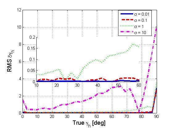
J. Mar. Sci. Eng. 2020, 8, 205 8 of 22
water,v a , and the ground speed, v g , represented by the velocity with respect to the inertial frame. The
velocity triangle is given by
v a = v g − vc , (4)
where vc is the velocity of the water current. The velocity triangle in Equation (4), projected into both
vertical and horizontal planes, is presented in Figure 2a,b.
The connection between the velocity vector expressed in the b-frame and the velocity vector
expressed in the c-frame is vc = T c,b · vb , or
vc cα c β sβ sα c β vbx
0 = −cα s β cβ −sα s β vby . (5)
0 −sα 0 cα vbz
From Equation (5), we can express the angle of attack with the body velocity vector components as
α = arctan(vbz /vbx ) , (6)
as well as the sideslip angle with both the body and water current velocity components,
β = arcsin(vby /vc )0 . (7)
2.4. Principle Component Analysis (PCA)
The method of PCA is mostly used to dilute the number of dimensions within a given set of
observations while still maintaining most of the information. The dimension reduction is possible if
the rank of the observations’ covariance matrix can be reduced. Geometrically, the PCA rotates the axis
of the original coordinate system into a new orthogonal axes, such that the new axes correspond to the
direction of maximal variability of the observations. This is performed statistically by an orthogonal
transformation to convert a set of observations of possibly correlated variables (which hence can be
diluted) onto a set of linearly uncorrelated variables called principal components. This transformation
is defined in such a way that the first principal component has the largest possible variance and that
each succeeding component, in turn, has the highest variance possible, under the constraint that it is
orthogonal to the preceding components. The resulting vectors form a set of uncorrelated orthogonal
bases. In other words, the principal components are eigenvectors of the symmetric covariance matrix,
and are thus orthogonal.
Applying the PCA to the accelerometer outputs from the inertial measurement unit, we find the
acceleration in the moving direction, thereby estimating the vertical directional angle. We perform
PCA through eigenvalue decomposition of a data covariance as follows. Let A be a matrix consisting
of acceleration measurements for a defined time span ∆t, such that each row i, Ai = a x (i ) ay (i ) az (i ) ,
of A is the measured acceleration vector at the ith time epoch. The covariance of A is defined by
PA = E[( Ai − E[ Ai ]) ( Ai − E[ Ai ])T ]. (8)
Given the data covariance, the corresponding eigenvectors, VA , can be calculated from the
eigenvalue problem
PA VA = VA PΛ , (9)
where each column is an eigenvector of PA . Finally, the PCA matrix is obtained by projecting A using
VA such that
APCA = VA · A . (10)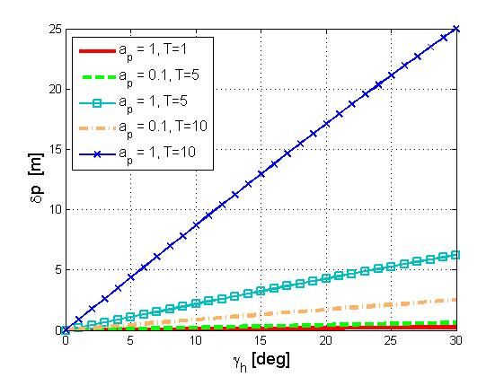
J. Mar. Sci. Eng. 2020, 8, 205 9 of 22
3. Applying the PCA Approach for Underwater Navigation
In this section, we describe our PCA-DR method to estimate the directional angles, γh and γh
from Figure 1a,b, respectively, by applying the PCA method using only accelerometer measurements.
The main concept of PCA-DR is that, instead of forming the velocity triangle to estimate the sideslip
angle and/or the angle of attack, we employ the same principles on an acceleration triangle.
3.1. System Model
Our considered system is comprised of one small submerged drifter, which is affected by
an acceleration force operating in a vertical and/or vertical angles with respect to the b-frame. This
force is related to a water current. We assume that both the drifter’s motion direction and the above
acceleration force are constant throughout the time the DR is performed; that is, for short time
periods between two successive position updates, the acceleration force experienced by the drifter is
time-invariant. We justify this assumption by the fact that, in most cases, the water current is a slow
varying phenomena. Still, since turbulence that causes rapid changes in the water current may occur,
we limit our approach to short term position tracking between successive position fixes, on the order
of a few seconds. We argue that, even in places such as coves where turbulence exists, these remain
time-invariant for such a short duration. This goes inline with the DR calculation, which is always
performed over short time intervals. We further assume that the drifter is moving in a straight line in
its body-frame such that the angular velocity experienced by the platform is negligible. The drifter is
equipped with accelerometers whose output is a timely three-dimensional specific force measurement
vector. The accelerometers frame is assumed fixed with respect to the b-frame, and the angle of the
accelerometer’s coordinate system with respect to the b-frame is assumed known. The drifter may be
equipped with a gyrocompass or a magnetometer, but we assume that these are of low accuracy and
cannot be used to measure the directional angles. Since DR simply integrates acceleration readings
accumulated over a time window, to operate our system we do not require the initialization of both
acceleration and velocity, and the operation is completely blind to the scenario’s setup.
Our aim is to perform DR in order to estimate the drifter’s position after a certain number of
acceleration measurements has been collected. While this period may induce some delay, it is only
an initial delay, and the DR can be performed over a sliding window. We measure the performance of
PCA-DR as a function of the estimation error,
ρ γh = |γh − γ̂h | (11)
ρ γv = |γv − γ̂v | , (12)
and the position error, q
2
ρp = ( p x (t) − p̂ x (t))2 + py (t) − p̂y (t) , (13)
where γ̂h and γ̂v are the estimation of the directional angles, and p(t) and p̂(t) are the drifter’s position
at time t and its estimate, respectively.
3.2. Estimating the Directional Angles
The transformation from the acceleration vector in the body frame ab = [ abx aby abz ] T onto the
acceleration of the PCA output, a PCA = [ a p 0 0] T , is established according to Equation (5), such that
ap c γv c γ h s γh s γv c γ h abx
0 = − c γv s γ h c γh −sγv sγh aby . (14)
0 − s γv 0 c γv abz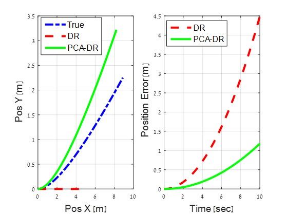
J. Mar. Sci. Eng. 2020, 8, 205 10 of 22
Note that, since we assume that, for the short time period that DR is performed, the angular
velocity that the platform experiences can be neglected, the Euler, Coriolis, and centrifugal accelerations
are not addressed in Equation (14).
The three axes’ accelerometer provides the specific force vector, fb = [ f x f y f z ] T , which is defined
as the acceleration vector a subtracted by the gravity vector g. If the submerged device’s pitch, θ,
and roll φ angles are known (i.e., the angles between the body and navigation frames), then the gravity
vector in the navigation frame gn = [0 0 g] T can be expressed in the body frame by
x x − sin(θ )
gb = x cos(θ ) sin(φ) gn
x
x cos(θ ) cos(φ)
x
− sin(θ ) gbx
= cos(θ ) sin(φ) g = gyb . (15)
cos(θ ) cos(φ) gzb
Given the gravity vector expressed in the body frame (from Equation (15)) and accelerometer
readings in the body frame fb = [ f x f y f z ] T , we have (recall that we assume negligible
angular velocities)
ab = fb + gb (16)
Substituting Equation (16) into Equation (14), we can calculate the values of γv and γh such that
!
f z + gzb
γv = arctan , (17)
f x + gbx
and
f y + gyb
γh = arcsin( ). (18)
ap
In this work, we consider the case that the drifter’s motion is mostly affected by the water current,
i.e., further from the influence of surface waves. In turn, except in rare cases, e.g., in the presence of
internal waves or hot water cooling fast, the water current mostly affects the drifter in the horizontal
plane. Thus, practically, the drifter’s motion is stable with negligible pitch and roll angles. Then, from
Equation (15), we conclude that the gravity vector expressed in the body frame is equal to the one
expressed in the navigation frame gbx = gyb = 0. Hence, Equation (16) can be further expressed as
fx
ab = fb + gb = fy , (19)
fz + g
and Equation (14) is modified to
ap c γv c γ h s γh s γv c γ h fx
0 = − c γv s γ h c γh − s γv s γ h f y . (20)
0 − s γv 0 c γv fz + g
From the last equation in Equation (20), we have
0 = − sin(γv ) f x + cos(γv )( f z + g) . (21)
In simpler terms,
fz + g
γv = arctan . (22)
fxJ. Mar. Sci. Eng. 2020, 8, 205 11 of 22
Since gyb = 0, Equation (18) reduces to
γh = arcsin( f y /a p ). (23)
Notice that the purpose of estimating the directional angles, γh and γv , is to perform DR relative
to an initial point. In order to implement this approach, theoretically, the pitch and roll angles must be
known to compensate for the accelerometer outputs regarding the gravity. Yet, if the platform’s roll
and pitch are small (a small angle approximation, say below 1 degree), then gbx and gyb can be neglected
in Equation (17) and Equation (18), and the calculation of γv and γh , respectively, can be performed
using only the platform accelerometers. Indeed, this is the case of drifters submerged below the reach
of surface waves. In the following, we derive the DR solution. To simplify the analysis, we consider
only horizontal DR using the estimation of γh . If needed, the same steps can then be taken to also
perform vertical DR using the estimation of γv .
4. PCA-DR Navigation
In this section, we present our derivation for our PCA-DR solution in the horizontal plane and
analyze the effect of errors in the estimation of γh . PCA-DR navigation is applied relative to an initial
point. Recall that we assume the underwater platform does not change its x b axis direction. That is,
during a determined time period TN for the DR calculation, â p and γh are considered constant. After
time TN , both â p and γh are recalculated and a new DR is performed. This process is illustrated in
Figure 4.
Figure 4. Illustration of the DR navigation process in the horizontal plane.
4.1. The DR Solution
Given the estimated acceleration in the moving direction, â p , and the directional angle, γh ,
the body accelerations are given by
ax = â p cos(γh ) ,
ay = â p sin(γh ) . (24)
Integrating Equation (24) yields the body velocity,
v x ( k + 1) = v x (k) + â p cos(γh )∆t ,
v y ( k + 1) = vy (k) + â p sin(γh )∆t , (25)J. Mar. Sci. Eng. 2020, 8, 205 12 of 22
and the drifter’s position is determined by
p x ( k + 1) = p x (k ) + v x (k )∆t ,
p y ( k + 1) = py (k) + vy (k)∆t . (26)
Recall that PCA-DR assumes an external acceleration-induced water current force. As a result,
PCA-DR should be operated when such force is identified. This can be done relatively easily
by observing the variability of the acceleration measurements. In particular, without an external
acceleration force, the output of the drifter’s accelerometers will be simply the gravity vector. In fact,
regardless of the drifter’s orientation, the magnitude of the gravity vector is fixed. When an external
acceleration force is present (i.e., a water current), the magnitude of the specific force, as measured by
the accelerometers, will have a different value than the gravity magnitude. Thus, the presence of the
water current can be determined by observing the differences between the measured acceleration and
the expected gravity vector.
4.2. Summary of PCA-DR Approach
The proposed PCA-DR approach flow chart is presented on the right side of Figure 5. The collected
accelerometer measurements (this is the raw data) are processed to produce Equation (13). Using the
PCA approach in Equation (9), we find the estimated acceleration in the moving direction a PCA .
Plugging this into Equation (13), we calculate the directional angles using Equations (16)–(18). Finally,
the PCA acceleration and directional angles are substituted into Equations (24)–(26) to obtain the
platform position.
Figure 5. Flow chart illustrating the differences between PCA-DR and traditional DR.
Figure 5 also highlights the key differences between our PCA-DR and the traditional DR. While
the latter performs DR based on an assumption of a straight line of another dynamic models, PCA-DR
uses the PCA technique over the acceleration measurements to estimate the directional angles and
to determine the moving direction. Note that PCA-DR should be operated when a water current
acceleration-induced force exists. As we explain later on, to identify such a force, the variability of
the acceleration measurements can be used. The moving direction largely depends on the magnitude
and direction of the water current and on the mass and shape of the drifter. Yet, in PCA-DR, we doJ. Mar. Sci. Eng. 2020, 8, 205 13 of 22
not calculate or directly measure the velocity of the water current, nor do we claim to calculate the
expected effect of the water current on the drifter. Instead, PCA-DR estimates the actual directional
angles formed by the water current. Further, avoiding the use of an assumed dynamic model that
otherwise may limit the application, PCA-DR integrates actual accelerometer measurements—after
compensation for the water current-induced directional angles.
4.3. Impact of Errors in Estimating the Directional Angles
The PCA-DR process described above depends on the estimation of both a p and γh . We now
present an analysis for the effect of estimation errors on the accuracy of the DR solution. Let us first
rewrite Equations (24)–(26) in state-space continuous form, such that
px 0 1 0 0 px 0
d vx 0 0 0 0 vx a p cos(γh )
= + . (27)
dt py 0 0 1 0 py 0
vy 0 0 0 0 vy a p sin(γh )
We assume that, during the DR period, a p and γh are constants. Hence, for the estimation errors
δa p for a p and δγh for γh , a linearization of v x in Equation (27) yields an estimation error,
δv̇ x = δa p cos(γh ) − a p sin(γh )δγh = C1 δa p − C2 δγh , (28)
where the constants are C1 = cos(γh ) and C2 = a p sin(γh ). Similarly, the estimation error of vy in
Equation (27) can be expressed by
δv̇y = δa p sin(γh ) + a p cos(γh )δγh = C3 δa p + C4 δγh (29)
where C3 = sin(γh ) and C4 = a p cos(γh ). Observing Equation (28) and Equation (29), we define the
error state model with the position and velocity states and augment it with the errors in the acceleration
and directional angle as
δp x 0 0 1 0 0 0 δp x
δpy
0 0 0 1 0 0
δpy
d δv x 0 0 0 0 C1 C2 δv x
= . (30)
dt 0 0 0 0 C3 C4
δvy δvy
δa p 0 0 0 0 0 0 δa p
δγh 0 0 0 0 0 0 δγh
Solving Equation (30) gives
∆t2 C1 ∆t2 C2
∆t
δp x 1 0 0 2 2 δp x0
∆t2 C3 ∆t2 C4
∆t
δpy 0 1 0 δpy0
2 2
∆tC1 ∆tC2
δv x
= 0 0 1 0 δv x0
.
(31)
∆tC3 ∆tC4
δvy
0 0 0 1 δvy0
δa p 0 0 0 0 1 0 δa p0
δγh 0 0 0 0 0 1 δγh0
Observing Equation (31), we see that the position errors diverge over time, due to the DR
nature of the problem, and their magnitudes depend on the initial conditions of the position, velocity,
and performance of the proposed approach, in terms of the initial acceleration and horizontal heading
directional angles.J. Mar. Sci. Eng. 2020, 8, 205 14 of 22
5. Analysis and Results
In this section, we report results from numerical and field work performance investigation. In all
cases, due to the limitation of DR to perform navigation over long periods of time, we consider only
short time intervals of a few seconds from the last navigation update. Further, since the water current
on the vertical axis is usually weak (accept in the rare cases of being affected by an internal wave or
in areas where hot water is cooling down) and since our PCA-DR approach is suitable for cases of
significant water currents, in our investigation we consider the private case of a water current acting
on the submerged platform in the horizontal plane such that γv = 0 while γh is non-zero.
5.1. Numerical Investigation
We now show a simulative investigation of the performance of PCA-DR. We employ a 1000
Monte-Carlo runs in which γh is uniformly randomized over a range of [0, π/2]. Unless mentioned
otherwise, in each simulation, γh , p x , and py are estimated over a navigation period of TN during
which 50 acceleration measurements are obtained. The acceleration noise for the three dimensions,
â p , is randomized according to a zero-mean i.i.d. Gaussian distribution with a fixed variance, σ,
that is characteristic of the inertial sensor. The roll and pitch angles are assumed known and constant
throughout the DR period, so the gravity vector can be expressed in the body frame. For this case,
we use Equation (18) for the calculation of γh . According to the procedure described in Section 3, using
the acceleration matrix A, a p is calculated based on Equations (8)–(10).
The performance of estimating a p is given in Figure 6, where we show the average of the RMS
of the estimation error δa p at each time step for a given value γh with perfect initial conditions,
i.e., δγh = 0. As expected, we observe that δa p does not depend on γh . That is, for a δγh = 0,
the projection of the acceleration measurements in the body frame, only the stability-frame is error free.
Figure 6. Average of the RMS of δa p as a function of γh . Curves represent different accelerometers’
p
noise variance σ in units of µg/ (Hr). The inner plot zooms in an area of interest in the figure.
In Figure 7, we show the error δγh = γ̂h − γh in estimating the directional angle using
Equation (18). Here, we assume δa p = 0. We observe that, while δa p does not depend on γh , for large
values of the noise variance σ, error δγh does change with γh . This is because the estimation of γh in
Equation (18) depends not only on the acceleration measurements, but also on gyb . Nevertheless, for
p
reasonable values σ = 1 µg/ (Hr) [40], the change of δγh with γh is not significant, and an error of
less than 0.5deg is observed for up to γh = 70 degrees. To comment on the impact of the navigation
period TN on performance, in Figure 8, we change TN to obtain 150 acceleration measurements and
show the error δγh as a function of γh . An improvement of more than 50% for most values of γh
is observed.J. Mar. Sci. Eng. 2020, 8, 205 15 of 22
Figure 7. RMS of δγh as a function of γh . Curves represent different accelerometer variance values σ in
p
units of µg/ (Hr).
Figure 8. RMS of δγh as a function of γh . Use of 150 acceleration measurements. Curves represent
p
different accelerometer variance values σ in units of µg/ ( Hr ).
Next, we evaluate the performance of PCA-DR
q using the closed form expressions in Equation (31).
Numerical values for the position error δp = δp2x + δp2y are shown in Figure 9. Results are shown as
a function of the two error terms of the PCA-DR approach, namely, δa p and δγh . We examine a scenario
with true values of γh = 30 deg and a p = 0.09 m/s2 and for a navigation period TN . We collect 1000
acceleration measurements for data analysis. In Figure 9, the initial position and velocity errors were
nullified. Figure 9 also includes (solid line with marker) the performance of the traditional DR, that
is, when the directional angles are neglected. The results show that, without compensating for the
directional angles, the DR error is roughly 4.5 m. This positioning error depends only on the actual
water current acting on the drifter and, clearly, is not sensitive to the two error sources of PCA-DR.
This is the reason why the positioning error of the traditional DR remains constant in Figure 9. We also
observe the strong dependency between the positioning error of the traditional DR and the error in
estimating the directional angles. This result motivates the need for an accurate estimation of the latter.J. Mar. Sci. Eng. 2020, 8, 205 16 of 22
Figure 9. Numerical positioning error of the DR procedure.
To further illustrate the difference between PCA-DR and other DR approaches, we examine
the navigation performance for a single data point from Figure 9. We consider the case where
δa p = 0.001 m/s2 and δγh = 15deg and a scenario of 10s between two position updates. In the
DR implementation, we assume perfect knowledge of the initial position and velocity of the drifter.
The comparison between the navigation performance over time of the DR and the PCA-DR approaches
for this scenario is shown in Figure 10. On the left panel, we show the estimated position of the drifter
using the two approaches relative to the true position. Notice that, using the DR approach, the position
remains in a straight line. This is excepted due to the assumption of no water current. Differently,
the performance of the PCA-DR approach depends on the values of δa p and δγh . On the right panel
of Figure 10, we show the position error of the two approaches. We observe that PCA-DR offers
a significant improvement of the position error by more than 70% compared to that of the traditional
DR approach.
Figure 10. Comparison between traditional DR and PCA-DR. Left panel: actual position of the two
approaches relative to the true position. Right panel: position error of the two approaches.
Based on the above discussion, we claim that, when a water current exists, the traditional DR
approach fails, while PCA-DR retains good DR performance. We also observe that, due to overfitting,
when no water current exists, the performance of PCA-DR is inferior to that of the traditional DR.
However, the performance degradation is not substantial.J. Mar. Sci. Eng. 2020, 8, 205 17 of 22
The results of the comparison between PCA-DR and the traditional DR also highlight the
robustness of the former. This is because exploring different directional angles corresponds to either
different water current forces or different drifter designs.
5.2. Experimental Investigation
In our simulations, we assumed that γv = 0 and that the water current induces an acceleration
force that results only in a non-zero γh . To test the validity of these assumptions, and to demonstrate
the performance of PCA-DR in a realistic scenario, we performed a designated sea experiment.
The experiment was conducted on December 2018 across the shoreline of Haifa. The water depth was
roughly 12 [m]. The sea conditions can be characterized as Beaufort force Level 1, and a significant
water current of roughly 1 knot was present. Together with the north–south direction of the Eastern
Mediterranean sea current, the area of the experiment is affected by two main local water current
sources originating from the nearby Haifa harbor and from the estuary of the nearby Kishon river.
The experiment involved in a single submerged water-proof tube including an industrial-graded
VectorNav vn-300 INS. The specifications of the INS includes a 5◦ per hour gyro in-run bias and a 0.04
mg accelerometer in-run bias. Only the VectorNav accelerometers are used for the experiments. Those
are indeed better than the ones found, for example, in our smartphones. Further, we did not calibrate
for sensor biases nor filter out the noises; rather, only the raw measurements were used. For the
examined time period (1–10 s), this is almost identical to taking low-cost sensors after bias calibration.
We used the INS at a rate of 10 [Hz], and recorded its data for offline processing. The tube was
lowered by scuba divers to the middle of the water current, and was then released to freely drift.
To have the tube maintain its depth, weights were carefully added to the drifter by the scuba divers.
Ground truth information about the location of the drifter was obtained by having the divers follow
the tube (without effecting its motion) while dragging a buoy with a GPS logger. As the direction and
magnitude of the water current in the tested area highly varied in space, this procedure was performed
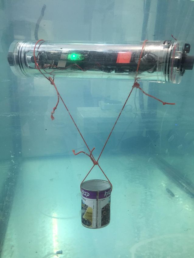
a few times to test the performance of PCA-DR for different water current conditions. A picture of the
deployed tube is shown in Figure 11.
Due to the limitation of the acceleration-only DR approach to perform tracking until the navigation
error drifters, we conducted sea experiments for very short time periods of a few seconds. Specifically,
we consider eight trajectories for our evaluation, with a minimum time duration of 3 s and a maximum
of 10 s. First, we examine the directional angle accuracy followed by DR analysis. To calculate the actual
direction of the tube, we used the GPS start and end points measured position, while the estimated
direction is obtained from the PCA analysis. Results are summarized in Table 1. For a short time
duration, an error of 0.02◦ was obtained, and for the 10 [s] trajectory, an error of 2.55◦ was obtained.
This result emphasizes the strength of the PCA-DR approach since, in regular DR, the direction cannot
be estimated.
Further, in Figure 12, we show the trajectory estimate of the drifter using our PCA-DR approach,
and compare it to the performance of the traditional DR approach that does not take into account
the water current. We note that, in both approaches, only acceleration data is used. Two trajectories
are shown for 3 s (Figure 12a,b) intervals, and the ground truth start and end positions are marked.
The ground truth was determined using the GPS receiver onboard the buoy. For both trajectories,
we observe that the traditional DR completely fails to follow the path of the drifter, and highly drifts
both in terms of the heading angle and in terms of the traveled distance. Due to the significant water
current, this drift starts already from the beginning of the motion. Contrarily, we observe that PCA-DR
successfully follows the path of the drifter, and manages to accurately calculate its heading angle.
This result supports the analysis shown in Figure 10. Notice that the GPS receiver used for ground
truth has a 5 m error; thus, the starting point of the trajectory is expected to have this range of error. Yet,
what is important is the behavior of the two approaches: the DR solution shows a traveled distance
of tens of meters (which of course was not the case), while our PCA-DR approach shows a traveledJ. Mar. Sci. Eng. 2020, 8, 205 18 of 22
distance of a few meters. Our point is that, while ground thruthing was not accurate, given the
outcome, we argue that our approach well outperforms classical DR.
(a) (b)
Figure 11. Pictures of the deployed drifter with the self-made INS in the test tank (a)) and at sea (b)).
Table 1. Directional angles recorded from the sea experiments.
Time [s] 3 4 5 6 7 8 10
True angle [deg] 0 2.03 2.04 2.35 2.34 2.81 2.89
PCA angle [deg] 0.02 1.57 1.59 1.60 1.57 1.64 0.34
Error [deg] 0.02 0.46 0.45 0.75 0.77 1.16 2.55
5 80
DR
70 PCA-DR
4 DR Start
PCA-DR 60 End
3 Start
End 50
2 40
Y[m]
Y[m]
1 30
20
0
10
-1
0
-2 -10
-0.01 0 0.01 0.02 0.03 0.04 -5 -4 -3 -2 -1 0 1
X[m] X[m]
(a) (b)
Figure 12. Results from the sea experiment comparing PCA-DR with the traditional DR approach.
(a) Trajectory A. Data collected for 3 s. (b) Trajectory B. Data collected for 10 s.J. Mar. Sci. Eng. 2020, 8, 205 19 of 22
In addition, using Equation (13), we calculated the position error at the end of the trajectories for
both regular DR and PCA-DR. The results are plotted in Figure 13. As expected, the DR solution error
drifts with time much more quickly than the PCR-DR approach. For the 10 s trajectory, the DR has
a position error of 76.6 m, while the PCA-DR has an error of 5.8 m. While this error may seem high,
we note that DR is performed over short periods of time before obtaining location fixes. Still, the focus
of our work is on considering induced acceleration force on the drifter, so the results should be
considered with respect to performing DR without such consideration. Here, the performance in
Figure 13 shows a huge improvement.
Figure 13. Position error results from the sea experiment comparing PCA-DR with the traditional DR
approach.
5.3. Discussion
Without a water current acting on the drifter, DR methods will give a satisfactory performance
between two successive position updates. Yet, as we show by the results of Figures 9 and 12,
for scenarios including an acceleration-induced water current force, even for short periods of time of
a few seconds, traditional DR approaches will result in large position errors. These errors dramatically
grow as a function of the time between position updates and the magnitude of the water current
acceleration force. In this respect, whenever the water current is substantial, it must be considered
in the DR process. Indeed, as we showed in numerical simulations and as we demonstrated in our
sea experiment, in such cases, PCA-DR performance far exceeds that of the traditional DR approach.
However, relying only on acceleration measurements, PCA-DR is limited to short time periods of
a few seconds. It should therefore be used within navigation fixes as an aid to either evaluate the
water current, or gap time instances without navigation assistance from, e.g., DVL. The accuracy of
PCA-DR depends on the accelerometer grade, the number of measurements used in the process of PCA
evaluation, and the value of the actual directional angle. In that context, the performance improvement
of PCA-DR might be obtained by analyzing the optimal number of acceleration measurements required
for the PCA evaluation. Further, PCA-DR can be extended for situations where the drifter also
experiences a vertical directional angle.
6. Conclusions
In this paper, we considered the problem of DR navigation for submerged drifters. These devices
drift with the water current to measure the current’s velocity or to observe certain phenomena. Hence,
they are not connected to, e.g., a surface buoy, but rather drift freely in the water column. Due to
their non-negligible size and shape, they are under the influence of an acceleration-driving force by
the water current. The water current affects the horizontal and vertical angles between the x-bodyYou can also read