Transition radiation based transverse beam diagnostics for non relativistic ion beams
←
→
Page content transcription
If your browser does not render page correctly, please read the page content below
Transition radiation based transverse beam
                                                           diagnostics for non relativistic ion beams
arXiv:2104.08487v1 [physics.ins-det] 17 Apr 2021

                                                               R. Singh∗1 , T. Reichert1 and B. Walasek-Hoehne1
                                                          1
                                                            GSI Helmholtzzentrum für Schwerionenforschung GmbH,
                                                                               Darmstadt, Germany
                                                                                      April 20, 2021

                                                                                          Abstract
                                                              The usage of optical transition radiation for profile monitoring of rel-
                                                          ativistic electron beams is well known. This report presents the case
                                                          for beam diagnostic application of optical transition radiation for non-
                                                          relativistic ion beams. The angular distribution of the transition radiation
                                                          emitted from few target materials for ion beam irradiation is shown. In
                                                          addition to expected linearly polarized transition radiation in the plane of
                                                          observation, a large amount (≈ ×20) of unpolarized radiation is observed
                                                          increasing towards grazing angles. The unpolarized radiation has the
                                                          characteristics of transition radiation and is understood as the transition
                                                          radiation generated from a ”strongly” rough target surface. This increase
                                                          in amount of radiation towards the detector can be used advantageously
                                                          towards transverse profile measurements and potentially other beam pa-
                                                          rameters. Further systematic effects such as the dependence of light yield
                                                          on beam current, comparison of the measured transverse profiles with Sec-
                                                          ondary electron emission based grid (SEM grid), target heating etc. are
                                                          also shown.

                                                   1      Introduction
                                                   Transition radiation is generated over a wide frequency range when a charged
                                                   particle traverses two different media. The existence of transition radiation
                                                   was first predicted by Ginzburg and Frank [1] where the expressions for the
                                                   radiated spectral intensity with the far field angular distribution were derived.
                                                   The radiation intensity is typically evaluated between two homogeneous media
                                                   with different permittivities such as the vacuum-metal boundary which is often
                                                   the case for most practical realizations.
                                                      A common picture for visualizing transition radiation for the case of a planar
                                                   vacuum-metal interface is the following. As the charged particle approaches the
                                                       ∗ r.singh@gsi.de

                                                                                               1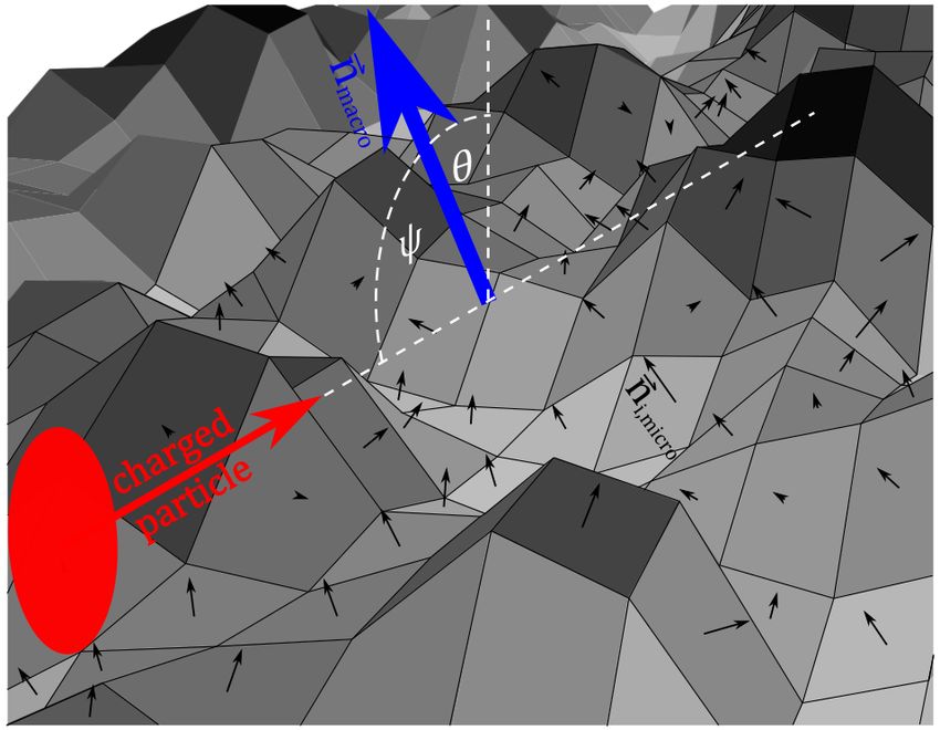
interface from the vacuum side, the coulomb fields associated with the charge
are terminated on the metal such that the boundary conditions are satisfied by
the induced polarization. However, when the charge hits the metal vacuum-
metal interface, the boundary conditions can only be satisfied with addition of
radiating electromagnetic fields which is referred to as transition radiation [2]. A
similar process happens on appearance of the charged particle through the metal
sheet on the other side at the metal-vacuum interface. The emitted radiation
is often separated as backward transition radiation (BTR) when the emission
is in the first medium and forward transition radiation (FTR) when it is in the
second medium. For non-relativistic ion beams, the beam is typically deposited
into the first few micrometers of the target and there is no forward transition ra-
diation expected unless very thin foils are used. One has to note, that although
simple descriptions for transition radiation are given for vacuum-metal inter-
face, transition radiation occurs at every material interface or by traversing an
inhomogeneous medium and is purely a surface phenomenon. With respect to
particle bunches another distinction commonly used in the jargon of transition
radiation is the coherent against incoherent transition radiation. The radiation
is referred to as coherent if the observed frequency range of the radiation is
contained in the frequency range of the source charge distribution. Coherent
transition radiation for optical frequencies would only occur for bunches with
temporal lengths in the order of few femto seconds (fs).

1.1    Optical transition radiation from smooth target.

                                            CCD
                                         ~ndet
                                ~kBT R

                      ~n
                                    θ                   ẑ
                                ψ
                           ~
                           βc
                                                             x̂

                Vacuum                       Radiator

        Figure 1: Charged particle beam impinging on a metal target

   Figure 1 shows the schematic of the particle trajectory, target or radiator
and the detector along with the relevant symbols. The co-ordinate system is
chosen in line with [3], i.e. the OTR target plane is defined as the x − y plane
and the target normal is towards the z axis. The plane of incidence consists of
                                             ~
                                             β
target normal ~n and beam incidence vector |β|  and the angle between them (ψ)

                                            2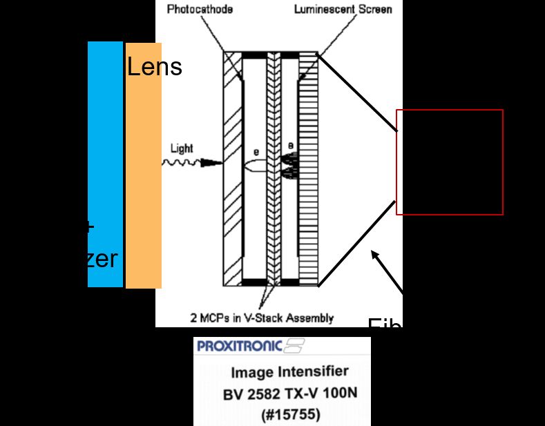
is referred to as the irradiation angle. The plane of incidence, in the shown case
co-incides with the x−z plane. The plane of radiation consists of ~n and radiation
wavevector kBT ~ R while the plane of observation contains beam incidence vector
β~ and the detector position n~det .
    In our designed experimental set-up with a smooth target, the beam inci-
dence vector, the target normal and detector position vector are in the same
plane, i.e. the plane of incidence and plane of observation co-incide. Further,
since only the radiation in the plane of observation is detected due to a small
                                       ~ R
acceptance of the detector (i.e. |kkBTBT R |
                                             ≈ n~det ), the relevant radiation vector
also lies in the same plane as incidence and observation plane.
    If an ion beam with a charge state Z is traversing from medium 1 with
1 = 1 into a medium 2 with arbitrary relative permittivity 2 =  at an irradi-
ation angle ψ, the angular distribution of the far field spectral radiant intensity
with a polarization parallel to plane of radiation (p polarized) as a function of
irradiation angle and emission angle θ is given as [3],

           dIk (n, ω, θ, φ, ψ)             Z 2 e2 βz2 cot2 θ| − 1|2
                               =                                           kA||2        (1)
                 dΩdω            4π 3 0 c[(1 − βx cos θx )2 − βz2 cos θ]2
where,
                   p                                                      p
         (1 + βz       − sin2 θ − βz2 − βx cos θx ) sin2 θ − βx βz cos θx  − sin2 θ
  A=                          p                                  p
                   ( cos θ +  − sin2 θ)(1 − βx cos θx + βz  − sin2 θ)
                                                                                (2)
and, βx = β sin ψ, βz = β cos ψ and cos θx = sin θ cos φ.
    There is also a component polarized perpendicular to the plane of radiation
(s-polarized) I⊥ , however I⊥ ≈ Ik · β 4 It is thus expected to be negligible in
comparison to parallel component for lower energies relevant for our studies
β < 0.5. For smooth targets oriented as shown in Fig. 1, we expect the radiation
detected by the camera to be linearly polarized since the target normal (~n) lies in
the plane of observation. For rough targets, the situation can change drastically
since the target normal varies across the whole target depending on the specifics
of the target surface structure and the polarization of the emitted radiation will
change correspondingly. This also has consequences for the angular distribution
as discussed in next subsection. Fig 2(a) shows a polar diagram representing
the angular distribution given by Eq. 1 for a unit charge with velocity β =
0.15 incident normally on perfect electrical conductor (PEC) and a realistic
conductor i.e. Iron (Fe). Fig 2(b) shows the angular distribution for various
irradiation angles. Here the relative permittivity of Iron at 500 nm was used
which can be found in [6]. The peak of the radiation for an iron target is at
θ ≈ 60◦ irrespective of the angle of irradiation ψ while for PEC, it is ψ = 90◦ .
The cumulative spectral intensity is highest for normal incidence onto the target.
    With this smooth surface assumption, optical transition radiation from low
electron beams have been already been observed [10, 11]. For low energy hadron
beams, usage of OTR for diagnostic purposes was proposed in 2008 [12]. Fol-
lowing which some pilot measurements were done, which confirmed the charge

                                              3
PEC
Iron
·10−40
ψ = 0◦
4.0 ψ = 30◦
ψ = 60◦
Beam 3.0
dIk (n,ω)
dΩdω
2.0
1.0
0.0
−90 −60 −30 0 30 60 90
Observation angle θ [◦ ]
(a) (b)
Figure 2: (a) Polar plot showing the angular distribution of transition radiation
emission from an Iron target in comparison to perfect electric conductor (PEC)
when irradiated by a singly charged particle with velocity β = 0.15 at ψ = 0. (b)
The angular distribution of spectral intensity for an Iron target when irradiated
at different angles.
state dependency of light yield. Spectroscopic investigations showed a broad-
band radiation indicating the presence of OTR were reported [13]. Polarization,
angular dependence and light yield were not studied in detail. Since the charge
state dependency also exists for other light producing mechanisms like beam
induced fluorescence (BIF), the data did not definitively confirm the measured
radiation as OTR in those pilot studies. This work tries to build upon that
experience.
1.2 Optical transition radiation from a rough target
An important concept for transition radiation generation is the ”effective source
size” ref f which for a certain radiation wavelength λ for a beam corresponding
to β is given as βγλ [9]. It is clear that for lower betas β < 0.5 and the radia-
tion emitted in optical regime, it is smaller than a naturally unprocessed surface
roughness. The targets used in this study were not controlled for surface rough-
ness and thus expected to have an rms roughness of ≥ 500 nm. This means
that each structure on the rough surface has the possibility to act as an individ-
ual radiator for transition and diffraction radiation with its own target normal
which might not co-incide with plane of observation. Another related √ concept
λβ 0
is the so called formation zone [3] and is given by, Lf ormation = 2π(1−β 0 cos θ)
√
4where 0 is given as (1 +2 )/2. Formation zone is comparable to the wavelength
and should not play a role in optical regime for smooth targets with low energy
beams. However, for rough targets, it can come into play where radiation can
be different from shallow and deep grooves and could play a role for diffraction
radiation. The proportion of the polarized light measured in the plane of ob-
Figure 3: Schematic representation of a target with a rough surface hit by a
charged particle under shallow incidence. Given the depicted piecewise pla-
nar micro-surfaces (with individual normals ~ni,micro ) are bigger than the eff.
transversal extent of the incident electric field (reff = βγλ in vacuum) they can
be thought as individual TR sources
servation will thus be given by the relative distribution of microscopic target
normals ~nmicro of individual radiators with respect to the macroscopic target
normal ~nmacro which was earlier simply denoted as ~n (see Fig. 1). Figure 3
shows a schematic of a rough target surface. We assume that the target nor-
mals for individual micro-radiators are randomly distributed in the 2D angular
space with respect to nmacro~ and have no preferred direction, i.e. ~nmicro is
a random variable with respect to θ, φ with E[~nmicro ] = ~nmacro where E[] is
the expectation operator. However, only the subset of micro-radiators normals
(~nmicro,OT R ) matter for OTR generation, i.e. the ones which can be irradiated
by the beam and E[~nmicro,OT R ] = ~nmacro +α. The value of α will depend on the
exact nature of the surface structure, if we assume a simple step or groove type
of structures on the surface, α ≈ π/2. The red blob shows the field distribution
of the charged particle and depicts the effective source size.
5A further complexity for transition radiation produced by low beta beams
is the scattering of OTR light off the target surface and its diffraction at the
edges of micro-radiators since a large part of the radiation is directed close
to the target surface (see Fig. 2). Scattering of light from a rough surface
has been a subject of intensive study for many decades since all surfaces are
rough to some extent. The studies have mainly been performed either from
the material surface characterization perspective [14] or were efforts towards
building perfect mirrors [15, 16]. Broadly speaking, rough surfaces are typically
characterized as ”weak” or ”strong” rough surfaces based on the ”rms” rough-
ness and characteristic length (correlation length) with respect to the incident
light wavelength [16]. Strongly rough surfaces have characteristic lengths and
rms roughness larger than the wavelength of interest. Further details on sur-
face roughness and scattering can be found in these references and references
therein [15, 16, 17]. Together, the surface scattering and randomly distributed
radiator angles especially for strong surface roughness can be of major conse-
quence for the degree of polarization in the plane of observation as well as the
angular distribution.
There has been early theoretical [18] and experimental [19] work showing
differences in optical transition radiation photon yield and polarization for low
energy electron beams. These studies were mainly concerned with very shallow
angles ψ > 80◦ and assigned the increase in radiation at shallow angles to
diffraction radiation. Further, it is known from literature that scattering via
surface electromagnetic waves or surface polaritons is not expected to play a
major role for strongly rough targets [16]. Nevertheless, we have also considered
a non-metallic OTR radiator to ascertain the contribution of surface plasmons
for the detected radiation. It is also important to note that, for β < 0.5 it is
hardly possible to control target roughness on the scale of micro-radiator size
βγλ for optical wavelengths under heavy ion irradiation. Already by energy
deposition the ion bombardment will degrade the surface in this regime even
after a short period of time. Based on the considerations above, the angular
distribution, light yield and polarization of transition radiation as seen in the
plane of observation from the rough target are expected to deviate from that of
a smooth target.
2 Optical transition radiation and transverse di-
agnostics
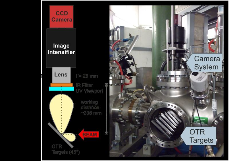
The experimental set-up is shown in Fig. 4. The metal targets used were 35 mm
wide and 100 mm high. Three metals were used, aluminium, stainless steel and
gold, where the former two were solid material of 2 mm thickness and the latter
was in form of a 1 µm thick layer sputtered on a 2 mm thick stainless steel
holder. Another target was a 5 mm thick disc (of diameter 110 mm ) made of
glassy carbon. All of them were attached to a target ladder with a stepper motor
based translation stage. A rotational stage was added to the ladder during the
6Figure 4: A set-up with a movable ladder with several OTR targets [13].
experiments, and therefore the absolute angle of the rotational element could not
be precisely calibrated. On the acquisition side, a 10 mm objective with 35 mm
focal length was placed roughly 36 ± 3cm above the target outside the vacuum
using a custom holder marked as ”camera system” in Fig. 4. Thus it covers a
solid angle ∆Ω ≈ 6 · 10−4 Sr. A linear polarizer was mounted directly in front
of the objective. The objective is followed by an image intensifier (Proxitronic,
Image intensifier BV 2582 TX-V 100 N), which was fiber coupled to a BASLER
CCD camera. The pressure in the vacuum chamber was measured to be about
5 · 10−7 mbar.
2.1 Expected number of photons in optical acceptance
from a smooth target and rough targets
First we estimate the total number of photons expected from backward tran-
sition radiation process in the backward half space. For a particle with given
charge state Z and velocity β, the total energy radiated in the frequency range
of interest ∆ω = ω2 − ω1 and half unit sphere on one side of the target can be
obtained be integrating the radiation intensity given in Eq. 1.
Z π Z 2π Z ω2
2 d2 Ik (n, ω)
Erad = · sin θdθdφdω (3)
0 0 ω1 dΩdω
Assuming a constant permittivity (see the validity of the assumption in Ap-
7·106
Photons generated from a smooth target
Photons generated from a smooth target
4 Eq. 3
2000 PEC
cos2 ψ
Iron
3 Gold
1500 Aluminium
Glassy Carbon
2
1000
1 500
0 0
0 20 40 60 80 0 20 40 60 80
Target normal with respect to beam axis (ψ) Target angle with respect to beam axis (ψ)
(a) (b)
Figure 5: (a)Total number of photons generated in ∆λ = 300 nm with center at
500 nm in the half sphere as a function of ψ for 5 · 109 Ca10+ ions. (b)Expected
number of photons in 6 · 10−4 sr from various target materials as a function of
beam incidence with respect to normal (ψ) at the observation angle θ = 90◦ −ψ.
pendix 5.3) over the frequency range and using the photon energy Eph = h̄ω
the number of photons per particle is approximated by
Z π
2
Z 2π Z 2
ω2 d Ik (n,ω)
dΩdω
Nph,t = sin θdθdφdω
0 0 ω1 Eph
ln ω2 Z π Z 2π
ω1 2 d2 Ik (n, ω)
= sin θdθdφ (4)
h̄ 0 0 dΩdω
Let us consider an example case of Ca10+ beam with energy corresponding
to β = 0.11 and an average current of 40 µA with 200 µs macropulse length
which in turn corresponds to Nion = 5 · 109 ions. As the spatial pulse length
is much bigger than the detected wavelenghts we scale Eq. 3 linearly with Nion
(incoherent sum) to find the total number of OTR photons generated by the
described macropulse normally incident on a steel target as ≈ 4 · 106 photons.
Due to unavailability of steel permittivity values, Iron permittivity is used for
the calculation and it is assumed that the wavelength range of acceptance of the
optical system is centered at 500 nm wavelength with ∆λ = 300 nm. Fig. 5(a)
shows the total photons generated as a function of beam incidence. A rough
estimate for total number of photons as a function of incident ion number Nions ,
energy and charge state impinging at an angle ψ with respect to normal on a
steel target can be given as,
Nph,t ≈ 7 · 10−4 · β 2 Z 2 cos2 ψNions (5)
8·104
35
Vertical Positon [mm]
Vertical Positon [mm]
30 1.5
25
20 1
15
10 0.5
5
(a) (b) (c)
0
0 5 10 15 20 25 0 5 10 15 20 25 0 5 10 15 20 25
Horizontal Positon [mm] Horizontal Positon [mm] Horizontal Positon [mm]
Figure 6: Transverse profile for Aluminum (top), Steel (middle) and Glassy
carbon (bottom) targets for same beam conditions corresponding to ψ = 50
degrees for 5 · 109 Ca10+ ions per macropulse. The plot is an average of 250
macropulses in stable low intensity machine conditions.
The actual number of photons which will make into the optical system with a
solid angle ∆Ω = 0.0006 Sr as a function of beam incidence is shown in Fig. 5(b).
Nion ∆Ω ω2 d2 Ik (n, ω)
Nph ≈ ln (6)
h̄ ω1 dΩdω
For a discussion on the number of photons required to form a transverse
profile image, see Appendix 5.5.
The conversion from well defined transition radiation generation process with
a given polarization and angular distribution to an isotropic and apparently
unpolarized source is governed by the surface roughness property and its in-
terplay with the angle of incidence ψ. To give some qualitative arguments on
the nature of this dependency, let us consider a simple rod based model for
the surface roughness. The amount of photons generated by this rod shaped
micro-radiator should have a similar scaling as smooth target, although shifted
by α which represents the difference between < ~nmicro,OT R > and ~nmacro in
the θ axis. α represents the slope of the rods with respect to target normal
resulting in a dependence of cos2 (ψ + α). These photons will be seen as un-
polarized in observation plane (φ = 0) since the ”rod” normal can be aligned
to any φ ∈ [−π/2, π/2]. Generally,the dependency of light yield from an actual
rough surface will differ from the qualitative picture discussed above and will
depend on the shape of individual radiators as well as their distribution and
separation. An accurate analysis requires a careful surface characterization and
is well outside the scope of this work. We will evaluate the dependency em-
pirically in the experimental data section. Further, one can expect that only a
certain proportion of generated photons from the micro-radiators will make into
the optical system due to scattering due to surrounding structures and an addi-
tional sin ψ dependence can be expected. This is similar to the optical system
9property ”Etendue” arising due to relative angle between the source and de-
tector. Apart from the aforementioned ”geometrical” factors; another potential
mechanism for dependence of the light yield as a function of irradiation angle
is the diffraction radiation and its role can become increasingly dominant as
ψ → π/2 as mentioned in [19]. If the charge travels close to the rough surface
without actually hitting it, a significant enhancement in the observed radiation
for grazing angles is possible. In case of periodic structures on the surface, a
peak in spectra corresponding to periodicity due to constructive interference of
the radiation can also be expected.
·108
1.2 Aluminum
Steel (V2A)
1.0 Glassy Carbon
CCD counts
0.8
0.6
0.4
0.2
0.0
0 10 20 30
Position [mm]
Figure 7: Beam profile in horizontal plane for Aluminum, Steel and Glassy
carbon targets for ψ = 50 degrees for 5 · 109 Ca10+ ions.
Figure 6 shows the two dimensional beam images from the transition ra-
diation for three target materials, Aluminum, Steel (V2A) and Glassy carbon
under the same beam and acquisition conditions. 5 · 109 Ca10+ ions was irra-
diated on the targets at an irradiation angle of ψ = 40 degrees. An average
over 250 images was performed to obtain the two dimensional images where
the colorbars are fixed to same values for all of the three images. The photon
count scaling trend for different target materials is similar to Fig. 5 (but not
the same) and is also visible in the profile heights of the horizontal projection
plotted in Fig. 7. The discrepancy is mainly for Steel target where we have used
permittivity values for Iron. The measured profile width is roughly the same
for all targets. We also see, that there is a saturated region on the Aluminum
target at the co-ordinates (20 mm, 20mm) (Fig. 6), and could be related to
macroscopic surface structure on the target. Similar less pronounced spots are
seen at (10mm, 22mm) and (25mm, 17mm) on the steel target. Another obser-
vation is that the background is proportional to the peak height, which hints
that the background might be primarily composed to scattered OTR photons.
The CCD count itself is a strongly non-linear function of intensifier volt-
age and cannot be directly correlated with the number of photons (discussed
in Appendix 5.1). However, for multiple measurements under the same beam
conditions, the CCD count fluctuation can provide an estimate of the aver-
10age number of photons generated. This would however be only true for lower
photon yields where the CCD count fluctuation is dominated by the statistical
fluctuation in the photon counts. This is discussed further in the Appendix 5.2.
2.2 CCD counts vs beam current
A systematic study to observe the relation between average beam current against
number of counts for the same intensifier and CCD settings. This study was
incidentally performed with a Gold target (Au) with Bismuth Bi26+ beam.
Figure 8 shows a single image for 200 µA beam current at ψ = 70 deg. The
background counts are subtracted by using the average pixel value from outside
the beam irradiation. This background region (BG) and region of interest (ROI)
ares annotated. An average beam current to CCD count dependence is shown
BG
50
Vertical Positon [mm]
40
30 ROI
20
10
0
0 10 20 30 40 50 60 70
Horizontal Positon [mm]
Figure 8: Individual image taken with a 80 µs gate for 200 µA Bi26+ beam
current. The rectangle marked on top left is used to subtract the background
counts per pixel.
in Fig. 9 (a). Each data point corresponds to a current transformer reading
and the corresponding image counts in the region of interest (ROI) for the
given macropulse. There is clear linear dependence between beam current and
CCD counts. Figure 9 (b) shows temporal correlation of the beam transformer
current and scaled CCD counts for ROI in the image for the same data as in
Fig 9. The conversion from photons entering the intensifier input to CCD counts
is discussed in the Appendix.
11Average Current [µA] and scaled counts [a.u]
·109
Integrated counts in ROI on ICCD Current Transformer
600 Scaled Counts
Data
Fit
1
400
0.5
200
0
0
0 100 200 300 400 500 600 0 5 10 15 20 25
Average pulse current [µA] Image Number
(a) (b)
Figure 9: (a) Macropulse average current vs integrated count per image in
the region of interest. A linear behavior from 40µA to 600µA (b) Current
transformer reading vs integrated counts on consecutive images for the four
current settings.
2.3 Polarization study
The dominant component of transition radiation due to a smooth target for
low beta beams is linearly polarized in the plane of radiation. This is one of
the signatures of transition radiation in comparison to other photon inducing
charged particle interactions like beam induced fluorescence (BIF) or material
luminescence. We measured images for different polarizer settings with respect
to plane of observation for a macropulse containing 5 · 109 Ca10+ ion beam
with velocity β = 0.11 irradiated on three target materials (Aluminum, Steel
and Glassy Carbon). One image was captured per macropulse. The MCP gain
was set to 1.726 V. Figures 10 and 11 shows 2D transverse profiles for ψ = 20
deg at six consecutive polarizer angles from a steel and glassy carbon target
respectively. The polarizer angle = 120◦ is when the polarizer axis is parallel
to plane to observation. These images were obtained by averaging 250 images.
The number of CCD counts are generally factor ≈ 2 higher for Steel target in
comparison to Glassy carbon target. There is a component which is polarized
in the plane of observation for both steel and glassy carbon target. Observing
linearly polarized radiation from both metallic and dielectric targets can be
considered as the evidence of OTR being a dominant radiation mechanism in
vacuum for the given beam conditions. It is also worth noticing that, in the
case when polarizer angle is perpendicular to the plane of observation (30◦ ),
there is still a significant amount of radiation left and the image corresponds
well to the beam profiles with other polarizer settings. This can be understood
as a consequence of the aforementioned surface roughness where the planes
of radiation of micro-radiators do generally not coincide with the one of the
macroscopic target. Therefore micro-radiators will effectively contribute to the
12·104
1.2
Vertical Positon [mm] 7.5
1
0.8
5
0.6
2.5 0.4
0.2
(a) (b) (c)
0
7.5
Vertical Positon [mm]
5
2.5
(d) (e) (f)
0
0 5 10 15 0 5 10 15 0 5 10 15
Horizontal Positon [mm] Horizontal Positon [mm] Horizontal Positon [mm]
Figure 10: Image with a steel (V2A) target at 20 degrees with respect to normal
at the polarization angle of (a) 0 (b) 30 (c) 60 (d) 90 (e) 120 and (c)150 deg.
photon yield which is unpolarized with respect to the plane of observation.
Figure 12(a) shows the average CCD counts for 250 images as a function of
polarization for an irradiation angle of ψ = 30◦ on an Aluminum target. The
polarizer angle was incremented in 30◦ steps at for each set of measurements
and covers the full 360 degrees. For N image measurements under the same
beam conditions, √ the error bar on the mean value of CCD counts is gives by
δcounts = σcounts / N . The polarization angles 120◦ and 300◦ correspond to the
plane of observation. The counts are accumulated for three different regions of
interest (ROIs). ROI 1 corresponds to the full image shown in Fig. 12(b). The
counts from ROI 1 are reduced by factor 10 for better visualization. ROI 2 and
3 are marked in the figure. They were chosen to avoid the ”hotspots” on the
image. These hotspots occur the at same location on the target irrespective of
beam movement, and therefore we suspect that they occur due to surface non-
uniformity forming some sort of a photon concentrator. There is no dependence
on the relative contributions of polarized to unpolarized light with the choice of
ROI. However, it is also worth noticing that in this specific case of Aluminum
for ψ = 30◦ , there is roughly a factor ≈ 8 more unpolarized radiation (since half
of unpolarized photons are blocked by the polarizer). The number of photons
from Aluminum target for steep angles ψ < 30◦ was saturating the CCD images
since most of the photons were hitting the few pixels exposed in the vertical
plane. Further, the Aluminum target has these hotspots exactly on the location
where beam was hitting as shown in Fig. 6. We have therefore not considered
the data from the Aluminum target for target rotation and angular distribution
studies discussed in the following section.
138,000
Vertical Positon [mm] 7.5
6,000
5
4,000
2.5
2,000
(a) (b) (c)
0
7.5
Vertical Positon [mm]
5
2.5
(d) (e) (f)
0
0 5 10 15 0 5 10 15 0 5 10 15
Horizontal Positon [mm] Horizontal Positon [mm] Horizontal Positon [mm]
Figure 11: Image with a Glassy carbon target at 20 degrees with respect to
normal at the polarization angle of (a) 0, (b) 30, (c) 60 (d) 90 (e) 120 and (f)
150 deg.
2.4 Light yield and angular distribution
Figures 10 and 11 showed the polarization for a fixed irradiation angle ψ =
20◦ . In the next step, we measured the radiation from several target angles
in the range ψ = 10 − 70◦ along with a systematic variation in the polarizer
settings covering 180 degree rotation in six steps. For a fixed polarizer angle,
Fig. 13 shows the beam image on a steel target as a function of ψ. The vertical
projection of the beam increases expectedly when the irradiation angle becomes
larger moving towards the grazing angle. Since the target was rotated, the
observation angle θ is correlated with irradiation angle θ = 90 − ψ and thus not
an independent parameter.
Figure 14 shows the fit separating polarized CCD counts and unpolarized
CCD counts vs polarization angle for several irradiation angles for Steel and
glassy carbon targets. In spite of the large error bars, the polarized components
could be fitted with the typical polarization curve and the peak at most irradia-
tion angles is seen at the polarizer angle of 120◦ when the polarizer axis coincides
with the plane of observation. A peculiar observation is that, at ψ > 60◦ , we
see a shift in polarization direction and an emergence of polarized photons per-
pendicular to the plane of observation. This observation suggests that the mean
of microscopic normal distribution < ~nmicro,OT R > varies as function of irradi-
ation angle and becomes perpendicular to the plane of observation for ψ > 60◦
resulting into a change of net polarization.
In Fig. 15, we have summarized the linearly polarized and unpolarized radi-
ation with respect to plane of observation as a function of irradiation angles for
steel and Glassy Carbon from the data shown in Fig. 14. The linearly polar-
14CCD Counts in the ROI normalized to beam current ·105
4 ROI 1 ·104
ROI 2
5
Vertical position [mm]
ROI 3
3.5 Fit
20 3
4
3 15
3
2.5 10
2
2
2 5
1
1.5 0
0 50 100 150 200 250 300 350 0 5 10 15 20 25
Polarization Angle Horizontal position [mm]
Figure 12: OTR light output from an Aluminum target as a function of polarizer
angle. 120 and 300 degrees on the polarizer corresponds to plane of incidence.
The different regions of interest for calculated counts are shown in the left figure.
ROI 1 corresponds to the shown full image while ROI 2 and ROI 3 are smaller
sections which are marked.
ized light in observation plane is compared with the scaled theoretical estimate
of photons shown in 5 as a function of ψ. The plots for the estimates are
normalized to match the measured sample for glassy carbon at ψ = 10. The
polarized light is seen when the charges hit the surfaces whose normal vectors
~nmicro,OT R lie in the plane of observation as expected from the macro normal
~nmacro . There is a rather good agreement for Glassy carbon data. For the
Steel target, the trend against ψ is correctly reproduced but the absolute es-
timate value has a notable discrepancy at ψ = 20◦ . As mentioned previously
the permittivity values for Iron were used to estimate the theoretical light yield
over irradiation angle to be compared to the Steel target. Even for Iron the
permittivity values given in literature have a rather large variation [4, 6, ?]. As
already discussed earlier, above ψ > 60, there are more micro-radiator surfaces
perpendicular to the plane of observation than the ones parallel to it giving a
net linearly polarized contribution in that direction.
The unpolarized component of radiation shown in Fig. 14(b) increases with
ψ and could be fit satisfactorily with the lowest order dependence of sin4 ψ.
Similar observations were also made for Gold and Aluminum targets. The
measured dependency is atleast an order higher than qualitatively argued i.e.
cos2 (ψ + α) sin ψ discussed in section 2.1. The increase in photon counts at
shallower angles (as ψ → π/2) can be a cumulative effect of many distinct
effects.
• The cos2 (ψ + α) dependence of generation process with the irradiation
angle.
• Lower scattering for the photons generated by micro-radiators at grazing
15·104
1.2
Vertical Position [mm]
25 1
20 0.8
15 0.6
10 0.4
5
0.2
(a) (b) (c)
0
Horizontal Positon [mm] Horizontal Positon [mm] Horizontal Positon [mm]
Vertical Position [mm]
25
20
15
10
5
(d) (e) (f)
0
0 5 10 15 0 5 10 15 0 5 10 15
Horizontal Positon [mm] Horizontal Positon [mm] Horizontal Positon [mm]
Figure 13: Image with a steel (V2A) target at (a) 10 (b) 20 (c) 40 and (d) 50
(e) 60 and (f) 70 degrees. with respect to normal at the polarization angle of
120 deg.
angles because the probability of shielding of photons by the generating
structure as well as rough neighborhood is reduced.
• An increase in the diffraction radiation is likely at grazing angles. This is
supported by another experimental observation, where we have observed
a large amount of radiation when the edge of targets were irradiated.
With diffraction playing a large role for shallow angle irradiation, a bound
dependency like sin4 ψ will most likely break down.
• Significant radiation at grazing angles is directed towards the target sur-
face which can be specularly reflected or scattered towards the detector,
resulting is further increase in light yield.
Given the data at hand, it is difficult to distinguish the dominant component
which results into the increased unpolarized radiation among all the effects
discussed above. Further, we have observed that under heavy ion irradiation, the
polarized components of radiation reduces further while unpolarized component
is unaffected. Faster surface deformation due to heavy ion irradiation might
reduce the polarized contributions arising from ~nmacro part of the target.
However the aforementioned observations support our working hypothesis;
i.e. a vast majority of the detected radiation on the CCD is indeed the optical
transition or diffraction radiation due to the target surface roughness. The
hypothesis is further strengthened by the measurements from the Glassy Carbon
which is a radiation-hard dielectric material. The material properties of Glassy
carbon allows no other generation mechanism like surface plasmons or metallic
16·106 ·106
2 ψ=70 ◦ ◦
60 ◦
50 40 ◦
20 ◦ ◦
10 1.2 ψ = 70◦ 60◦ 50◦ 40◦ 20◦ 10◦
CCD Counts in the ROI
CCD Counts in the ROI
1
1.5
0.8
0.6
1
0.4
0.5 0.2
0 20 40 60 80 100 120 140 0 20 40 60 80 100 120 140
Polarization Angle Polarization Angle
Figure 14: CCD counts as a function of incidence angle and polarization angle
for steel target (left) and Glassy carbon target (right).
oxide fluorescence. The yield for polarized, unpolarized and background light
scales expectedly with the permittivities of different target materials and hints
strongly that all the radiation (including background) is primarily transition
or diffraction radiation. From the transverse profile measurement perspective,
there are only two relevant questions; 1) Is the observed un-polarized radiation
a result of transition or diffraction radiation processes? 2) Does it represent the
exact transverse profile of the beam. Based on the data available, the answer
to both the questions is affirmative.
2.5 Comparison of OTR profile with SEM-Grid
A comparison between secondary electron emission monitor grid (SEM-Grid)
and OTR image which are longitudinally separated by 1 m is shown in Fig. 16
(a). This measurement was performed with 8.6 MeV/u 95 µA Ar18+ beam
irradiated on a steel target. The SEM-Grid wires are 2.1 mm apart and and in-
terpolation between the wires is performed by the SEM grid software. Generally
a good agreement between OTR images and SEM-Grid profiles is seen.
2.6 Counts a function of MCP gate delay
As part of the initial studies to rule out fluorescence and any other slow pro-
cesses, MCP gate was set to a fixed width (100 µs) and the measurement was
triggered at different delays with respect to beam macropulse arrival. This mea-
surement was performed with 11.4 MeV/u 20 µA F e25+ beam with a macropulse
length of 1 ms. The coarsely sampled pulse shape was reconstructed with this
measurement in 13 delay steps as shown in 16 (b).
17Estimate for Iron
4 25 Unpolarized Steel
Estimate Glassy Carbon
Relative Counts/Intensity
Unpolarized Glassy Carbon
Relative Counts/Intensity
Polarized Steel
Polarized Glassy Carbon 20 sin4 ψ fit
3
15
2
10
1
5
0 0
0 20 40 60 80 0 20 40 60 80
Target normal with respect to beam axis Target normal with respect to beam axis
(a) (b)
Figure 15: (a) Detected polarized photons from steel (V2A) and Glassy carbon
target as a function of polarizer and target angle. (b) Unpolarized photons from
steel (V2A) and Glassy carbon target as a function of polarizer and target angle.
2.7 Target heating and thermal photons
The number of OTR photons per image are in the order of 20-1000 for low
intensity beams discussed in this report. Therefore profile imaging using OTR
is sensitive to any thermal photons resulting from target heating. An estimate
of thermal photons per unit frequency f and solid angle Ω as a function of target
temperature can be obtained by Planck’s law,
dIT (n, f ) 2hf 3 1
= 2 · hf /K T (7)
dΩdf c e B −1
Fig. 17 shows the dependence of the number of photons generated as a function
of target temperature for radiation centered in different parts of the spectra
within 200 nm spectral width. One can see a threshold like behavior; i.e. when
the temperature of target crosses a certain threshold, thermal photons with
longest wavelengths allowed by the optical system will start to interfere with
the measured profile image. As can be seen that already at 700 K temperature,
photons centered at 500 nm photons can overwhelm the OTR based profile
image. This behavior was observed with a 400 uA current Bi26+ beam as shown
in Fig 18(a). There was no optical filter applied for this specific measurement.
Using a ICCD gating period of 70 us, the beam profile is not distorted while
with a gate of 100 us, the central part of the image is dominated by thermal
photons. This concludes that the center of the target with beam crosses the
temperature threshold in about 70 us from the start the of macropulse. Target
heating can be counter-acted by depositing the beam energy of a larger surface
area of the target as shown in Fig. 18(b), where under exactly the same beam
conditions as Fig. 18(a), no heating is observed. Since a larger area of the target
was under irradiation, the target did not cross the temperature threshold to
generate enough thermal photons. Thermal photons can be reduced by utilizing
18·105
1.2 OTR from Steel target 1.5
Counts in 0.1 ms time intervals
SEM Grid
1
Normalized Counts
0.8
1
0.6
0.4 0.5
0.2
0 0
−15 −10 −5 0 5 10 15 0 0.2 0.4 0.6 0.8 1.0 1.2
Position [mm] Time [ms]
Figure 16: (a) Comparison of a horizontal profile from secondary electron
emission grid (SEM-Grid) and OTR light for a Ar18+ beam with 95 µA and
100 µs pulse length. (b) The mean count for F e25+ beam with 20 µA average
current in a 1 ms macropulse for 100 µs MCP gate width with a varing delay
marked on the x-axis. The error bars are calculated from count fluctuations
over 100 macropulses.
either shorter macropulses, shallower target angles, infrared filters or active
target cooling. As shown in Fig. 17, application of optical filters which cut out
photons above 300 nm can allow the target temperature to increase upto 1100-
1200K without any significant thermal photon disturbance. For most practical
measurements in our current range of upto few mA, target heating should not be
an issue if marcopulse length is controlled or an optical filter is applied. However,
target heating always needs to be considered in an OTR based diagnostics for
low energy hadron beams.
3 Summary and applications
We have shown that the OTR for ion beams provides enough photons for the
measurement of a beam profile covering the typical range of intensities in accel-
erator operations. The light yield and polarization differs significantly between
an ideal smooth target and the rough targets as observed experimentally. Rough
targets has enhanced radiation at grazing angles, which can lower the intensity
and energy thresholds for usability of the OTR process in hadron beam di-
agnostics. It also opens up possibilities for optimization of camera angles for
beam imaging, non-destructive profile monitoring and energy deposition on a
larger surface area to avoid target heating. There are few immediate applica-
tions, the first is the construction of a SEM-Grid like profiler that will allow
SEM-Grid like diagnostics especially since the light emissions from the edges
of the wires (grazing incidence) can be quite high. It could be advantageous
for transversally small high intensity beams, since construction of SEM-Grids is
19103
102
Thermal photon counts
101
100
10−1
300 nm
10−2 400 nm
500 nm
10−3
400 600 800 1000 1200
Target temperature [K]
Figure 17: Thermal Photons.
particularly challenging in those cases. The second use case is the modeling of
non destructive devices like ionization profile monitors (IPM) and beam induced
fluorescence (BIF) monitors under high beam intensity. The IPM and BIF mon-
itors are known to be affected by direct beam fields (space charge) and OTR
can provide an in-situ non space charge affected profile for correction and mod-
eling. Eventually, with the usage of very thin foils (< 0.5 µm) such that beam
traverses without significant energy deposition, transverse profile measurements
can be combined with bunch length measurements using recently demonstrated
GHz transition radiation based bunch length monitor [21] to obtain a fast, non-
destructive and compact full 6D emittance measurement set-up. Finally, OTR
with thin radiation hard materials like Silicon carbide (SiC), Glassy Carbon,
Carbon stripper foils (already used at GSI [23]), Zinc Oxide (ZnO) in high en-
ergy beam transport opens up a possibility for an almost non-destructive profile
monitoring especially for fully stripped particles. The light yield after the syn-
chrotrons should be high enough to be observed on a normal CCD directly.
Although the results presented in this paper are promising in context of
typical transverse profile measurement, there is still work to do towards theo-
retical modeling (in line with [18]) at least for simpler surface structures [20],
and experimental verification of the results as a function of surface roughness
and irradiation angle on light yield. An evaluation of the precision of the profiles
measured with unpolarized component of the transition radiation in context of
scattering from rough surfaces and changes in surface due to effect of heavy ion
bombardment is also required. This is relevant for detailed beam profile mea-
surements for high intensity beams such as halo measurements or measurements
of very narrow beams (< 1 mm). There are other potential applications e.g.
if rough surfaces and multiple radiators could produce more than one photon
per ion for high energy beams; non destructive OTR based particle counters for
high energy beams can be foreseen.
2050 50
Vertical Positon [mm]
Vertical Positon [mm]
40 40
30 30
20 20
10 10
0 0
Horizontal Positon [mm] Horizontal Positon [mm]
50 50
Vertical Positon [mm]
Vertical Positon [mm]
40 40
30 30
20 20
10 10
0 0
0 10 20 30 40 50 60 70 0 10 20 30 40 50 60 70
Horizontal Positon [mm] Horizontal Positon [mm]
Figure 18: Image with a 70 us gate (top) and 100 us (bottom) from the beginning
of the macropulse for 400 uA current for target incidence ψ = 25 deg.Image with
a 70 us gate (top) and 100 us (bottom) from the beginning of the macropulse
for 400 uA current for target incidence of ψ = 65 deg.
4 Acknowledgment
C. Andre, A. Ahmed, P. Forck, M. Mueller and S. Udrea are acknowledged
for multiple discussions and help in mechanical set-up. GSI Target laboratory
colleagues for providing the stripper foils and GSI Material science department
colleagues for providing Glassy carbon target for these experiments are also
gratefully acknowledged. Finally, we thank the UNILAC operations crew for
their support during the experiments.
References
[1] V. L. Ginzburg and I. M. Frank, “Transition radiation,” Zh. Eksp. Teor.
Fiz. 16, 15–22 (1946).
[2] V. L. Ginzburg and V. N. Tsytovich, Transition Radiation and Transition
Scattering (Adam Hilger, New York, 1990).
[3] M. Ter-Mikaelian, High Energy Electromagnetic Processes in Condensed
Media (Wiley/Interscience, New York, 1972).
21[4] M. A. Ordal, L. L. Long, R. J. Bell, S. E. Bell, R. R. Bell, R. W. Alexander,
Jr., and C. A. Ward, Optical properties of the metals Al, Co, Cu, Au, Fe,
Pb, Ni, Pd, Pt, Ag, Ti, and W in the infrared and far infrared. APPLIED
OPTICS / Vol. 22, No.7 / 1 April 1983.
[5] F. Cheng, P.-H. Su, J. Choi, S. Gwo, X. Li, C.-K. Shih. Epitaxial growth of
atomically smooth aluminum on silicon and its intrinsic optical properties,
ACS Nano 10, 9852-9860 (2016)
[6] P. B. Johnson and R. W. Christy, Optical constants of transition metals:
Ti, V, Cr, Mn, Fe, Co, Ni, and Pd, Phys. Rev. B 9, 5056-5070 (1974)
[7] M.W. Williams and E.T. Arakawa, Optical properties of glassy car-
bon from 0 to 82 eV, Journal of Applied Physics 43, 3460 (1972);
https://doi.org/10.1063/1.1661738.
[8] G. M. Garibyan, ”Transition radiation effects in particle energy ”, J. Exptl.
Theoret. Phys. (U.S.S.R.) 37, 527-533 (August, 1959)
[9] V. Verzilov, Transition radiation in the pre-wave zone, Phys. Lett. A 273,
135 (2000).
[10] C. Bal , E. Bravin, E. Chevallay, T. Lefevre and G. Suberlucq, OTR from
non-relativistic electrons, Part of Beam diagnostics and instrumentation for
particle accelerators. Proceedings, 6th European Workshop, DIPAC 2003,
Mainz, Germany, May 5-7, 2003
[11] R. B. Fiorito, D. Feldman, A. G. Shkvarunets, S. Casey, B. L. Beaudoin, B.
Quinn, and P. G. O’Shea, “OTR measurements of the 10 kev electron beam
at the University of Maryland electron ring (UMER),” in Proceedings of
Particle Accelerator Conference (IEEE, 2007), pp. 4006–4008.
[12] A. Lumpkin, Feasibility of OTR imaging of non-relativisitc ions at GSI.
Scintillator screen workshop, GSI.
[13] B. Walasek-Höhne, C. Andre, F. Becker, P. Forck, A. Reiter, M. Schwickert,
and A. Lumpkin, Optical transition radiation for non-relativistic ion beams,
in Proceedings of the High-Intensity and High-Brightness Hadron Beams,
Beijing, China, 2012 (JACoW, Geneva, 2012), THO3C01,p. 580.
[14] William S. Bickel, Richard R. Zito, and Vince Iafelice, Polarized light scat-
tering from metal surfaces, Journal of Applied Physics 61, 5392 (1987);
[15] J. Ingers, M. Breidne , Surface roughness scatterning theories - A numerical
comparison”, Proc. SPIE 2019, Scattering and diffraction, (28 March 1989);
doi:10.1117/12.950433.
[16] A. A. Maradudin and E. R. Mendez, Light scattering from randomly rough
surfaces, Volume: 90 issue: 4, page(s): 161-221 Issue published: October
1, 2007, https://doi.org/10.3184/003685007X228711.
22[17] A. Marvin, F. Toigo, and V. Celli, Light scattering from rough surfaces:
General incidence angle and polarization, Phys. Rev. B 11, 2777 – Published
15 April 1975.
[18] R. A. Bagiyan, Transition radiation from rough surfaces, Acta Physicae
Superficierum, Vol 2, (1990).
[19] F. R. Arutyunyan, A. Kh. Mkhitaryan, R. A. Oganesyan, B. 0. Rostomyan,
and M. G. Sarinyan, Polarization and spectral composition of the radiation
of nonrelativistic electrons interacting with a rough surface, Zh. Eksp. Teor.
Fiz. 77, 1788-1898 (November 1979).
[20] J. E. Rutkowski, Transition radiation emitted from a surface irregularity
shaped as rectangular step and rectangular groove, Acta Physicae Super-
ficierum, Vol 2, (1990).
[21] R. Singh and T. Reichert, Analytical calculations and CST Simulations for
a transition radiation based longitudinal charge profile monitor, manuscript
under preparation.
[22] C. Andre, P. Forck, R. Haseitl, A. Reiter, R. Singh, B. Walasek-
Hoehne,Optimization of beam induced fluorescence monitors for profile
measurements of high current heavy Ion beams at GSI, TUPD05 Proceed-
ings of IBIC2014, Monterey, CA, USA.
[23] Barth, W., Kaiser, M.S., Lommel, B. et al. Carbon stripper foils for
high current heavy ion operation. J Radioanal Nucl Chem 299, 1047–1053
(2014). https://doi.org/10.1007/s10967-013-2651-3
[24] Steven D. Johnson, Paul-Antoine Moreau, Thomas Gregory, and Miles J.
Padgetta, How many photons does it take to form an image? Appl. Phys.
Lett. 116, 260504 (2020); https://doi.org/10.1063/5.0009493
5 Appendix
5.1 Transmission and conversion with the optical system
onto the CCD
Figure 19 shows the components of the optical system. The optical system
consists of few parameters, a) Quantum efficiency of the photocathode, b) MCP
voltage and resulting electron multiplication (gain) and c) Phospor converting
the electrons back to photons which are detected on the CCD. Photocathode
quantum efficiency spectral response for the given system is presented in the
table below:
23Figure 19: Optical system
wavelength (nm) sensitivity (mA/W) QE (%)
200 22.0 13.7
220 23.8 13.4
240 25.8 13.3
260 31.8 15.1
280 37.5 16.6
300 31.5 13.0
320 34.5 13.3
340 39.0 14.2
360 41.6 14.3
380 45.5 14.8
400 49.0 15.2
450 51.0 14.1
514 39.0 9.4
650 21.0 4.0
800 0.2 0.0
Total number of photons detected at the CCD as a function of pho-
tons entering the ICCD: Photocathode: QE at 400 nm = 0.15 , i.e. 0.15
el/ph. 10-15% of the incoming photons are detected. If the MCP gain of 1.2
kV is applied; 3000 el/el result; similary for 1.6 kV = 300000 el/el. (See man-
ual/slides). Phosphor 46 provides 90 ph/el at 6 KV (default voltage between
MCP and Phosphor). Thus the total input to output photon conversion at MCP
gain 1.2 kV(≈ 4 · 104 ) and 1.6 kV (≈ 4 · 106 ) ph/ph.
The quantum efficiency of the Basler 311F CCD camera is not yet clear. The
default pixel values without beam was 500±60 (in 2 byte mode). Thus there are
247 effective bits allowing a dynamic range of 40 dB (factor 100). The intensifier
was aimed to be used in photon counting mode, i.e. a high gain around 1.4
kV was set where each photon detected on the photocathode resulted in 106
photons on the CCD making a ”blob”. This set-up is only appropriate for low
photon scenario (≤ 50 photons per image) at smaller values of ψ. We noticed
CCD saturation for individual images for Aluminum target at ψ = 10◦ and 20◦
during our measurements with 6.0 MeV/u 5 · 109 Ca10+ ions.
5.2 CCD count fluctuations
An independent way of estimating the number of photons reaching the CCD
is to evaluate the fluctuations in the number of counts for consecutive images
under the same beam and target conditions under constant beam conditions.
These type of discrete event number related fluctuations are referred to as ”shot”
noise in electronics literature and is modelled by a Poisson process.
For a Poisson process with an√average of N events in a given time interval,
the shot noise is expected to be N . Beam current is measured independently
using a current transformer and was 40 ± 1 µA for the discussed data. The
beam current fluctuations contribute very weakly to the count fluctuations since
σI σcounts
. Based on this data itself, it is not clear if the fluctuations
are dominated by the noise in image intensification process or the photons gen-
eration process, however it does allow an estimate on the lower bound on the
number of events reaching the CCD. Assuming that the fluctuation is count rates
is dominated by the shot noise of the generated photons, the average number
of events or generated photons can be estimated as
< counts > 2
Nph,average = (8)
σcounts
Figure 20 (a) shows the fluctuations in the CCD count for irradiation of Alu-
minum target for several incidence angles. The estimated photon counts are
shown in Figure 20 (b). We have to note that, the role of background subtrac-
tion is crucial for this process since this is an absolute photon number estimate.
For ·109 Ca10+ beam with β = 0.11., we estimate generation of 1000 photons for
Aluminium target at ψ = 30◦ (Fig. 5. As discussed in 5.1, the photocathode has
an average quantium efficiency of 15%, and the optical system should register
a maximum of ≈ 150 photons per image from a smooth target. On the other
hand, the photon estimate from the measurements is from a rough Aluminum
target, and the maximum intensity (140 photons) is measured at ψ = 70.
In comparison to photon yields above, the beam induced fluorescence mon-
itor provides roughly ≈ 50 times lower number of photons when scaled for the
same beam conditions [22]. As discussed above, 500 events or photons are suf-
ficient to provide a reliable 1 D profile for an image intensified system.
25·108
2
ψ = 70 60 50 40 20 10
140
CCD Counts in ROI
Estimated photon yield
1.5
120
100
1
80
0.5 60
40
0 50 100 150 200 0 20 40 60 80
Image Number Beam irradiation angle ψ
(a) Permittivity (b) ψ = 10
Figure 20: CCD counts from Aluminum target for various irradiation angles
when the polarizer angle is set to 0◦ .
5.3 OTR spectra for Iron, Aluminum and Glassy carbon
It is clear from Eq. 1 that the transition radiation spectral intensity is a rather
complex function of material permittivity, angle of irradiation and angle of
observation. For low betas, e.g. (β·10−40
40
Iron Iron
Aluminum Aluminum
4
Glassy Carbon Glassy carbon
30
3
dIk (n,ω)
00
+ j
dΩdω
20
2
0
10 1
0
0
0.35 0.40 0.45 0.50 0.55 0.60 0.65 0.35 0.40 0.45 0.50 0.55 0.60 0.65
Wavelength [µm] Wavelength [µm]
(a) Permittivity (b) ψ = 10
·10−40
·10−41
5 Iron
Iron
Aluminum 2
Aluminum
4 Glassy carbon
Glassy carbon
1.5
3
dIk (n,ω)
dIk (n,ω)
dΩdω
dΩdω
2 1
1 0.5
0
0
0.35 0.40 0.45 0.50 0.55 0.60 0.65 0.35 0.40 0.45 0.50 0.55 0.60 0.65
Wavelength [µm] Wavelength [µm]
(c) ψ = 40 (d) ψ = 70
Figure 21: Optical transition radiation spectra. (a) Shows the variation in
absolute value of epsilon in visible range. (b-d) Calculated radiated spectral
intensity for different irradiation angles and the observation angle is θ = 90 − ψ.
27with the result obtained using spectral energy ([2])
!
dE Z 2 e2 1 + β2 1+β
= ln −1 (10)
dω 4π 2 0 c 2β 1−β
which is valid for normal incidence and PEC. In the latter case the total photon
number is given as
Nion ω2 dE
Nph,PEC,⊥ = ln (11)
h̄ ω1 dω
For Nion = 5 · 109 ions with charge state Z = 10 travelling with β = 0.11 and
in the wavelength range λ ∈ [350, 650] nm one obtains 1.166 · 107 photons using
(11). This gives a scaling of Nph,t = 2 · 10−3 β 2 Z 2 Nions inline with Eq. 5.
5.5 Number of photons needed for profile measurement
Modern detectors are capable of detecting every photon which are registered as
an electron on the input of an MCP or PMT due to their large amplification.
Therefore the question of the number of photons required to form a profile image
has moved towards the source [24]; how many photons should be emitted to
obtain a reasonable beam profile image? The answer to this question depends
on the resolution requirements. If we want a 2-D beam image with a cross
section of 15 mm × 15 mm with 0.5 mm spatial resolution and an amplitude
resolution of 3% or 30 levels (5 bits). The total degrees of freedom for this
problem are Ndf = 30 × 30 × 30 = 27000. Since the absence or presence of a
photon convey information to a binary bit, the total number of photons required
is Nph,t,2D = Ndf /2 = 13500.
For obtaining 2 1-D projections of the profile, the requirements are much
meagre, Nph,t,1D = Nph,t,1D /15 ≈ 1000. Such a requirement can easily be
fulfilled for the typical intensities at heavy ion and proton linacs.
5.6 Long term irradiation
Figure 22 shows two images spaced by an interval of half an hour of high in-
tensity beam irradiation on Gold target. Approximately ≈ 1013 Bi26+ ions for
irradiated on the target in this time interval. No change in the measured beam
profile is observed.
28You can also read