A high-resolution image time series of the Gorner Glacier - Swiss Alps - derived from repeated unmanned aerial vehicle surveys
←
→
Page content transcription
If your browser does not render page correctly, please read the page content below
Earth Syst. Sci. Data, 11, 579–588, 2019
https://doi.org/10.5194/essd-11-579-2019
© Author(s) 2019. This work is distributed under
the Creative Commons Attribution 4.0 License.

                   A high-resolution image time series of the
                     Gorner Glacier – Swiss Alps – derived
                from repeated unmanned aerial vehicle surveys
              Lionel Benoit1 , Aurelie Gourdon1,2 , Raphaël Vallat1 , Inigo Irarrazaval1 , Mathieu Gravey1 ,
                 Benjamin Lehmann1 , Günther Prasicek1,3 , Dominik Gräff4 , Frederic Herman1 , and
                                                 Gregoire Mariethoz1
               1 Institute
                         of Earth Surface Dynamics (IDYST), University of Lausanne, Lausanne, Switzerland
                   2 Ecole
                         Normale Supérieure de Lyon, Département des Sciences de la Terre, Lyon, France
                     3 Department of Geography and Geology, University of Salzburg, Salzburg, Austria
              4 Laboratory of Hydraulics, Hydrology and Glaciology (VAW), ETH Zürich, Zürich, Switzerland

                                  Correspondence: Lionel Benoit (lionel.benoit@unil.ch)

                               Received: 27 November 2018 – Discussion started: 10 December 2018
                             Revised: 6 April 2019 – Accepted: 17 April 2019 – Published: 30 April 2019

       Abstract. Modern drone technology provides an efficient means to monitor the response of alpine glaciers to
       climate warming. Here we present a new topographic dataset based on images collected during 10 UAV surveys
       of the Gorner Glacier glacial system (Switzerland) carried out approximately every 2 weeks throughout the
       summer of 2017. The final products, available at https://doi.org/10.5281/zenodo.2630456 (Benoit et al., 2018),
       consist of a series of 10 cm resolution orthoimages, digital elevation models of the glacier surface, and maps of
       ice surface displacement. Used on its own, this dataset allows mapping of the glacier and monitoring surface
       velocities over the summer at a very high spatial resolution. Coupled with a classification or feature detection
       algorithm, it enables the extraction of structures such as surface drainage networks, debris, or snow cover. The
       approach we present can be used in the future to gain insights into ice flow dynamics.

1   Introduction                                                    al., 2015) and remotely sensed data acquired from diverse
                                                                    platforms: ground-based devices (Gabbud et al., 2015; Pier-
Glacier ice flows by deformation and sliding in response to         mattei at al., 2015), aircraft (Baltsavias et al., 2001; Mertes
gravitational forces. As a glacier moves, internal pressure         et al., 2017), or satellites (Herman et al., 2011; Kääb et al.,
gradients and stresses create visible surface features such         2012; Dehecq et al., 2015; Berthier et al., 2014). Recently,
as glacial ogives and crevasses (Cuffey and Paterson, 2010).        the development of unmanned aerial vehicles (UAVs) has
Furthermore, the surface of glaciers is also shaped by local        enabled glaciologists to carry out their own aerial surveys
weather conditions, which are responsible for the snow ac-          autonomously, rapidly, and at reasonable costs (Whitehead
cumulation and ablation. Related processes generate distinct        et al., 2013; Immerzeel et al., 2014; Bhardwaj et al., 2016;
morphologies such as supraglacial streams, ponds, and lakes.        Jouvet et al., 2017; Rossini et al., 2018). This technology is
   Glacier surface features evolve continuously, and these          particularly attractive to map alpine glaciers whose limited
changes provide insights into the structure, internal dynam-        size allows a satisfying coverage at a centimeter to decimeter
ics, and mass balance of the glacier. Important efforts have        spatial resolution.
been made to monitor glacier surfaces, from early stakes               Here we provide a homogenized and high-resolution
measurements at the end of the 19th century (Chen and Funk,         remote-sensing dataset covering about 10 km2 of the ablation
1990) to present-day in situ topographic surveys (Ramirez et        zone of the Gorner Glacier glacial system (Valais, Switzer-
al., 2001; Aizen et al., 2006; Dunse et al., 2012; Benoit et        land, Fig. 1). The raw images have been acquired by UAV

Published by Copernicus Publications.
580                                                 L. Benoit et al.: A high-resolution image time series of the Gorner Glacier

flights carried out approximately every 2 weeks during the         ous crevasses. The entire Gorner Glacier system (i.e., the ter-
summer of 2017 (from 29 May to 30 October). The dataset            minal tongue and its five tributaries) covers an area of almost
comprises 10 consecutive digital elevation models (DEMs)           50 km2 and its central flow line is 12 km long, making it one
and associated orthomosaics of the area of interest at a 10 cm     of the largest European glaciers (Sugiyama et al., 2010).
resolution. It is therefore one of the most exhaustive surveys        The Gorner Glacier system has been widely studied since
of the short-term surface evolution of a temperate glacier         the 1970s due to its significant size, its accessibility, and
currently available. Geometrical coherence of the dataset          because a glacier-dammed lake threatened the downstream
is ensured through the application of comprehensive pho-           Matter valley with glacier outburst floods (Sugiyama et al.,
togrammetric processing (i.e., images are ortho-rectified and      2010; Werder et al., 2009, 2013). The long history of glacio-
properly scaled). In addition, the orthomosaics are stackable      logical studies in this area has shown that the mass balance
thanks to a co-registration procedure. The dataset can there-      of the Gorner Glacier system was stable from the 1930s to
fore be seen as a high-resolution time lapse of the Gorner         the early 1980s, and significantly dropped since then (Huss
Glacier ablation zone, combining spectral (orthomosaics)           et al., 2012). This can be associated with the rise of its equi-
and geometrical (DEMs) information on the glacier surface.         librium line altitude (ELA) due to an increase in the local
In addition to orthomosaics and DEMs that are snapshots of         average yearly temperature. The ELA is at around 3300 m to-
the area of interest, we also provide a product that we call       day according to studies carried out at the neighboring Findel
matching maps (MMs) to achieve temporal monitoring of the          Glacier (Sold et al., 2016).
glacier. In practice, a MM associates with each pixel of an or-       In this context, the current dataset aims at complementing
thomosaic (respectively a DEM) the corresponding pixel in          existing studies about the Gorner Glacier system by docu-
the next orthomosaic recorded 2 weeks later. MMs can then          menting the behavior of its ablation zone during an entire
be used to track the flow of ice over time, and in turn to quan-   summer, at a time when this glacial system is thought to be
tify ice surface displacements.                                    out of equilibrium with a clear trend toward glacial retreat.
   Potential uses of this dataset are numerous. Single ortho-      In particular, this dataset focuses on the monitoring of the
mosaics and DEMs can be used to map the surface of the             glacier surface at high spatial and temporal resolution.
glacier and to extract features of interest such as the sur-
face drainage network (Yang and Smith, 2012; Rippin et             2.2   UAV surveys
al., 2015), debris, or snow cover (Racoviteanu and Williams,
2012). Alternatively, the complete time series of orthomo-         The primary data are RGB images acquired by repeated UAV
saics and DEMs can be used for detection and quantification        surveys over an area of 10 km2 . A fully autonomous fixed-
of changes at the surface of the glacier (Barrand et al., 2009;    wing UAV of type eBee from SenseFly, equipped with a 20-
Berthier et al., 2016; Fugazza et al., 2018). Finally, the time    megapixel SenseFly S.O.D.A camera, has been used for im-
lapse coupled with the MMs is an interesting tool to moni-         age acquisition (Vallet et al., 2011). The camera was static
tor ice surface velocity and deformation (Ryan et al., 2015;       within the UAV body (no gimbal) and therefore all pictures
Kraaijenbrink et al., 2016), and in turn ice flow dynamics         are quasi-nadir (i.e., images are taken with an angle ±10◦
at the glacier surface (Brun et al., 2018). The MMs provide        from the vertical line). For flight planning and UAV piloting,
a quantification of the ice velocity at every location on the      the eMotion3 software was used.
surface of the glacier, which can be used to calibrate or to          Raw images were acquired with a ground resolution rang-
validate ice flow models, especially for the Gorner Glacier,       ing from 7.3 to 8.8 cm for the glaciated parts of the area of
which was extensively used as a modeling benchmark (see            interest. For the requirements of photogrammetric process-
for instance Werder and Funk, 2009; Riesen et al., 2010;           ing, flight plans have been designed to allow for an overlap
Sugiyama et al., 2010; Werder et al., 2013).                       between images ranging from 70 % to 85 % in the flight di-
                                                                   rection and from 60 % to 70 % in the cross-flight direction.
                                                                   These specifications have led to flight altitudes ranging from
2     Data acquisition                                             300 to 600 m above ground. The flight time was limited to
                                                                   about 30 min in field conditions. Thus, the coverage of the
2.1    Study site                                                  full area of interest required four to eight separate flights per
The Gorner Glacier is located in the Valais Alps in south-         session, i.e., each day of acquisition (Table 1). Overall, 10
ern Switzerland (Fig. 1a). It is part of a glacier system in-      sessions were conducted in 2017, from 29 May to 30 Oc-
volving five tributaries and ranges from 2200 to 4634 m a.s.l.     tober. The main features of these flights are summarized in
(Fig. 1b). The ablation area, which is the main focus of this      Table 1.
study, is a 4 km long and relatively flat ice tongue (slope
around 6 %, i.e., 3.4◦ ) that is deeply incised by meltwater
channels and partially debris covered (Fig. 1c). This ablation
area is preceded by a steeper part (southwest of the Monte
Rosa Hut, Fig. 1c) characterized by the presence of numer-

Earth Syst. Sci. Data, 11, 579–588, 2019                                            www.earth-syst-sci-data.net/11/579/2019/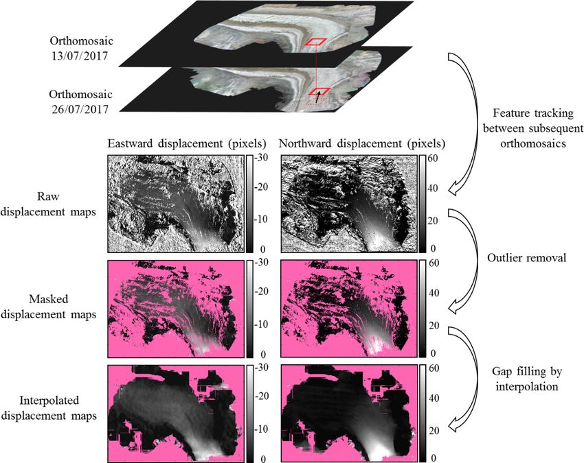
L. Benoit et al.: A high-resolution image time series of the Gorner Glacier                                                      581

Figure 1. The Gorner Glacier system. (a) Situation map. (b) Overview of the Gorner Glacier system; dashed red line: area of interest.
(c) Picture of the glacier tongue.

Table 1. UAV flights carried out for raw glacier image acquisition.      To improve the coherence of the co-referencing of the dif-
                                                                      ferent sessions, all products are co-registered to the reference
        Date           Acquisition time   No. of     No. of           of the 9 June acquisition (Fig. 2). To this end, the coordinates
                                 (CET)    flights   pictures          of several stable points of the landscape (16 to 70 among a
        2017/05/29         14:00–16:00         4        749           set of 74; see Table 2 and Fig. 4) are extracted from the bun-
        2017/06/09         12:30–15:30         8        935           dle adjustment of 9 June, and used as manual tie points for
        2017/06/21         11:30–13:30         7        930           the bundle adjustments of the other dates. These stable points
        2017/06/27         11:30–14:00         5       1059           are mostly salient features of the bedrock or erratic boulders
        2017/07/13         12:30–14:00         4        830           on the deglaciated banks of the glacier. The co-registration
        2017/07/26         13:00–16:00         6       1125           leads to orthomosaics and DEMs that are stackable. There-
        2017/08/15         12:30–16:00         7       1121           fore, in the final products, the bedrock remains stable be-
        2017/10/04         12:00–15:30         7       1107           tween consecutive dates, while the glaciated parts move and
        2017/10/18         13:00–15:00         4        846           deform. Consequently, if a time lapse is created from the
        2017/10/30         13:00–15:30         6       1084
                                                                      co-registered products, the glacier appears to flow while the
                                                                      surrounding landscape remains static. Figure 2 summarizes
                                                                      the acquisition and processing chain used to derive the final
3     Data processing                                                 products of the dataset.
                                                                         After co-registration, all final products (orthomosaics and
3.1    Generation of co-registered orthomosaics and                   DEMs) are in the reference frame of the bundle adjustment
       DEMs                                                           of 9 June 2017 (hereafter referred to as master bundle ad-
Pictures have been processed separately for each acquisition          justment). This local reference frame is a realization of the
date with the photogrammetric software pix4DMapper ver-               WGS84 reference system (with Universal Transverse Merca-
sion 3.1 (Vallet et al., 2011, Fig. 2) using default parame-          tor (UTM zone 32) projection) using code-only GPS data as
ters for nadir flights (see the processing reports for details        input for referencing. The absence of ground control points
about these parameters). The output resolution has been set           (GCPs) and the use of consumer-grade GPS observations in
to 10 cm per pixel in order to prescribe a constant resolution        the bundle adjustment procedure can result in meter-level
across all final products. During the photogrammetric pro-            geolocation errors and internal deformations of the master
cessing, the raw pictures are first oriented by bundle adjust-        bundle adjustment (James and Robson, 2014; Gindraux et
ment, and then a DEM and an ortho-rectified image (ortho-             al., 2017). While the internal deformations of the local ref-
mosaic) are generated for each day of interest. Since the only        erence frame lead to relative measurement errors of small
geolocation information included into the bundle adjustment           amplitude (on the order of 1/1000; see Sect. 4.1 for details),
procedure is the trajectory of the UAV derived from code-             the geolocation errors related to the absence of GCPs can
only GPS data, the initial geo-referencing of the orthomo-            impair comparisons with other datasets covering the same
saics and DEMs is limited to a few meters.                            geographic area. To improve absolute georeferencing and to
                                                                      link our dataset with the Swiss national reference system, Ta-
                                                                      ble 2 provides the parameters of the affine transformation be-

www.earth-syst-sci-data.net/11/579/2019/                                                Earth Syst. Sci. Data, 11, 579–588, 2019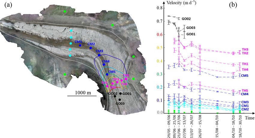
582 L. Benoit et al.: A high-resolution image time series of the Gorner Glacier
in the following orthomosaic (and therefore easily navigate
within the whole dataset).
The MMs are obtained by image matching of pairs of or-
thomosaics. The orthomosaic at time t is taken as a refer-
ence, and for each pixel of the reference, a 51 × 51 pixel
(5.1 m × 5.1 m) patch is extracted and searched for in the or-
thomosaic corresponding to the next session (time t + dt).
To speed up the processing and avoid wrong matches with
very distant patches, the homologous patch at time t + dt is
searched for in a neighborhood with a 200-pixel (20 m) ra-
dius centered on the position of the original patch at time
t whose size has been established based on prior knowl-
edge about the approximate surface velocity of the Gorner
Glacier. The criterion used to evaluate the similarity between
both patches is the mean absolute error (MAE) between pix-
els computed on grayscale images (Liu and Zaccarin, 1993;
Chuang et al., 2015). The MAE has been selected as the sim-
ilarity score because it is fast to compute, especially on large
images using convolutions. Its disadvantage is the sensitiv-
ity to illumination differences between consecutive orthoim-
Figure 2. Acquisition and processing chain used to derive the co- ages. However, in practice, no adverse effects have been ob-
registered orthomosaics and DEMs. served, mostly because the images were acquired roughly at
the same time of the day (between 11:30 and 16:00), and
Table 2. Parameters of the affine transformation between the Swiss because the orthoimages used to generate the MMs are al-
reference system (CH1903 – LV03) and the local reference frame ways separated by less than 1 month, which mitigates the il-
defined by the master bundle adjustment of 9 June 2017. Note that lumination differences. The patch of the image t +dt leading
no shear nor reflection is considered. Locations of the manual tie to the lowest MAE with the original patch at time t is then
points used to estimate the transformation parameters are shown in considered the counterpart of the original patch. Finally, the
Fig. 4. displacements (in pixels) between the two patches along the
east–west and the north–south directions are recorded into
Translation Translation Rotation Scale the MM. This operation is repeated for all possible patches
eastward (m) northward (m) (◦ ) in the reference orthomosaic. The MMs have been calculated
321 800.8 −5 009 609.3 1.1357 1.0004 using an open-source utility called MatchingMapMaker de-
veloped as part of this project, and made available along
with the dataset (see Sect. 5.2 for code availability). The
tween the local reference frame of this dataset and the Swiss MatchingMapMaker tool has been designed to account for
CH1903 – LV 03 reference system. This transformation has the specificities of UAV-based orthoimages, and in particu-
been estimated from 81 manual tie points identified in (1) the lar their very high resolution. To ensure the reliability of this
orthomosaic derived from the master bundle adjustment and utility, MMs have been benchmarked against horizontal dis-
(2) a 50 cm resolution orthomosaic of 2009 processed and placement maps calculated using well-established image cor-
georeferenced by the Swiss mapping agency swisstopo. relation algorithms, namely IMCORR (Scherler et al., 2008)
and CIAS (Heid and Kääb, 2012). The results of this bench-
mark (see Sect. 5.2) show a very good agreement between
3.2 Surface displacement tracking: generation of MMs
horizontal displacement maps derived from MatchingMap-
Consecutive co-registered orthomosaics enable us to quan- Maker, IMCORR, and CIAS.
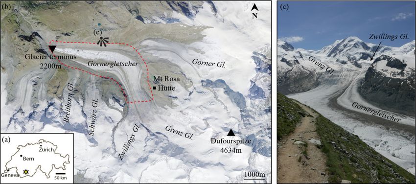
tify horizontal displacements at the surface of the glacier. In The raw MMs can be noisy due to the presence of outliers
the present dataset, this information about ice surface dis- in the pattern matching procedure (speckled areas in the raw
placements is provided by the MMs (Fig. 3). In practice, a displacement maps in Fig. 3). These outliers originate from
MM is an image that pairs the positions of similar ice patches the dissimilarity between subsequent orthomosaics, due to,
at times t and t + dt (dt being the time span between consec- for example, changing shadows or changes at the glacier sur-
utive acquisitions) (Fig. 2). The footprint of the MM is the face (snowfall, snow, or ice melting, etc.). To mitigate the
overlap of the footprints of the orthomosaics at times t and impact of these outliers, we first locate them, then we mask
t + dt. MMs inherit the spatial resolution of the original or- the impacted areas (pink areas in Fig. 3), and finally we in-
thomosaics (i.e., 10 cm) and can therefore be used to directly terpolate the remaining reliable displacements to fill the gaps
relate any pixel of a given orthomosaic to its counterpart generated by the mask. To limit the processing time, a sim-
Earth Syst. Sci. Data, 11, 579–588, 2019 www.earth-syst-sci-data.net/11/579/2019/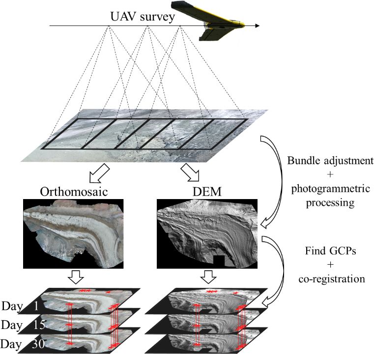
L. Benoit et al.: A high-resolution image time series of the Gorner Glacier                                                    583

plistic outlier detection method based on signal processing        between the observed and the modeled position of tie points
has been preferred over more sophisticated approaches based        used during the relative orientation step. The sub-pixel level
on glacier physics (Maksymiuk et al., 2016). Unreliable ar-        of errors (Table 2, column 2) ensures that the orientations of
eas in the raw MMs are assumed to be aggregates of pixels          the camera are reliable. Next, the co-registration step is as-
with spatially incoherent displacement values embedded in a        sessed by the mean root-mean-square error (RMSE) of man-
matrix of displacements that vary smoothly in space (i.e., the     ual tie point coordinates. This statistic measures the stabil-
reliable displacements). The borders of unreliable areas are       ity of manual tie point coordinates between different bundle
detected as locations with strong spatial displacement gra-        adjustments. Under ideal conditions, the value of the mean
dients, with a detection threshold set to 15 cm of horizontal      RMSE on manual tie points should be close to the ground
deformation per day. A mask of reliability is then created         pixel resolution of the raw images (i.e., 7.3 to 8.8 cm) be-
by setting the areas with a strong gradient to 0 and the re-       cause an operator is able to identify points of interest with a
mainder of the mask image to 1. The outlier areas (i.e., small     pixel level precision. The slightly higher values obtained in
aggregates of unreliable values) are then filtered out by ap-      the present case (9 to 21 cm, Table 2, column 3) can be due to
plying the opening operator of mathematical morphology to          the difficulty of precisely identifying manual tie points under
this mask with a structuring element of the size 50 × 50 pix-      changing environmental conditions (e.g., sunlight exposition
els. This operation leads to switch the value of the mask from     or snow cover). The errors in manual tie point identification
1 to 0 for all aggregates of pixels smaller than 50 × 50 pixels.   degrade the mean RMSE, but they are expected to have a
Hence, we obtain a mask with 1 at locations with reliable dis-     mild impact on the co-registration itself because they are not
placements and 0 where the measured displacements are con-         correlated and tend to compensate for each other. Note that
sidered outliers. Finally, the values of the MM at masked lo-      late in the season (i.e., for the last acquisition on 30 October)
cations are interpolated from the non-masked measurements          it became difficult to identify manual tie points due to strong
using a bilinear interpolation. The selected procedure is it-      shadows, hence the small number of manual tie points at that
erative. At each iteration, it attributes to the masked values     time.
the mean of the reliable values in a 500-pixel neighborhood           Another important validation consists of assessing possi-
in the east–west and north–south directions. The values that       ble internal deformations within the local reference frame
remain masked after 10 iterations are considered to be too         of the dataset. Figure 4a displays the residuals of the co-
far from the informed areas to be filled and are set to −99 to     registration of the master bundle adjustment on a georefer-
denote no data. Figure 3 summarizes how MMs are derived            enced orthoimage, which are a proxy for the internal defor-
from pairs of consecutive co-registered orthomosaics and fil-      mations of the master bundle adjustment. The results show
tered to remove outliers.                                          that the internal deformations have a meter-level amplitude
   Because MMs pair the positions of similar ice patches be-       (mean deformation = 1.07 m; max deformation = 2.83 m)
tween consecutive orthomosaics, they can be used to derive         and are smoothly spread over the area of interest due to the
maps of the horizontal displacements occurring at the surface      bundle adjustment procedure, which tends to distribute er-
of the glacier. To this end, displacements from the masked         rors over space. It follows that, considering the extent of
MMs are converted to meters per day and resampled at a 5 m         the study area (a few square kilometers), the relative error
resolution to remove the dependence between neighboring            induced by the internal deformations of the local reference
locations that is introduced during the image matching pro-        frame is on the order of 1/1000. Thanks to the co-registration
cedure. Horizontal displacement maps at 5 m resolution are         procedure, the internal deformations of all orthomosaics and
provided in addition to the full-resolution MMs in order to        DEMs are similar to the ones of the local reference frame
facilitate the use of the present dataset in the context of ice    defined by the master adjustment. When measuring changes
flow studies.                                                      at the surface of the glacier from the present dataset, the er-
                                                                   ror related to internal deformations is therefore on the order
                                                                   of 1 ‰ of the measured distances. This results in relatively
4     Quality assessment
                                                                   small absolute errors because the changes at the ice surface
4.1    Bundle adjustment and co-registration
                                                                   of the Gorner Glacier are of moderate amplitude (e.g., ice
                                                                   ablation reaches a few centimeters per day, and ice flows at
A first validation of this dataset can be performed by check-      less than 1 m d−1 in the ablation zone). For instance, in the
ing the relative orientation of the cameras during the bundle      case of horizontal velocity measurements, the order of mag-
adjustment, as well as the co-registration of orthomosaics         nitude of glacier displacement between two acquisition dates
and DEMs. Processing reports detailing the quality of the          is 30 cm d−1 × 14 d = 4.2 m. It follows that the error in ve-
bundle adjustment for each session are available along with        locity due to internal deformations is 4.2 m ×1/1000/14 d =
the dataset (see Sect. 5.1).                                       0.3 mm d−1 , which is very small in comparison with the am-
   Table 2 displays three indices summarizing the quality of       plitude of the ice surface velocity itself.
both bundle adjustment steps. First, the mean reprojection
error (in pixels) quantifies the mismatch in the raw images

www.earth-syst-sci-data.net/11/579/2019/                                             Earth Syst. Sci. Data, 11, 579–588, 2019
584 L. Benoit et al.: A high-resolution image time series of the Gorner Glacier
Figure 3. Processing chain used to compute a MM between two subsequent orthomosaics. The procedure is illustrated for the 13 July 2017–
26 July 2017 period. In displacement maps, masked areas are displayed in pink.
Table 3. Quality assessment of the bundle adjustment procedure.
Date Relative orientation: Co-registration: Co-registration:
mean reprojection error (pix) mean RMSE (m) no. of manual tie points
2017/05/29 0.138 0.210 66
2017/06/09 0.136 Reference Reference
2017/06/21 0.123 0.189 66
2017/06/27 0.146 0.193 68
2017/07/13 0.120 0.107 63
2017/07/26 0.117 0.206 70
2017/08/15 0.118 0.175 69
2017/10/04 0.125 0.122 38
2017/10/18 0.127 0.146 43
2017/10/30 0.125 0.092 16
4.2 Orthomosaics and DEMs the edges of the area of interest artifacts can be present due
to the low number of overlapping images in these areas (see
In addition to the bundle adjustment, we also validate the the processing reports to identify them). This leads to un-
final products of the photogrammetric processing (Fig. 4a), reliable photogrammetric reconstructions and in particular
i.e., the co-registered orthomosaics and DEMs. To this end, shear lines (Fig. 4d). Despite these relatively minor artifacts
individual orthomosaics and DEMs have first been visu- restricted to the edges of the surveyed area, all glaciated
ally checked to track the presence of artifacts. A careful parts and nearby unglaciated margins are satisfyingly recon-
examination of all products shows that the glaciated parts structed in both orthomosaics and DEMs.
(Fig. 4b) as well as the neighboring ice-free areas (Fig. 4c)
are well reconstructed in both orthomosaics and DEMs. On
Earth Syst. Sci. Data, 11, 579–588, 2019 www.earth-syst-sci-data.net/11/579/2019/L. Benoit et al.: A high-resolution image time series of the Gorner Glacier 585
4.3 MMs “mm” the month and “dd” the day of acquisition. Finally,
these sub-folders contain the following files:
In addition to the visual inspection of individual photogram-
metric products, we also assess the quality of the co- – 2017_mm_dd_orthomosaic.tiff: contains the orthomo-
registration procedure by quantifying in the MMs the stabil- saic.
ity of several areas that are most likely static, as well as the
– 2017_mm_dd_dem.tiff: contains the DEM.
observed spatial patterns of glacier surface velocity. We se-
lect several validation locations on and off the glacier (Fig. 5) – 2017_mm_dd_report.pdf: contains the processing re-
and compute their horizontal velocity by dividing the dis- port (generated by Pix4D Mapper) that summarizes the
placements recorded in the MMs by the time elapsed be- quality of the photogrammetric processing for the date
tween the acquisitions. Note that in Fig. 5 the velocity is av- of interest.
eraged over 10×10 m2 areas, corresponding to 10 000 single
measurement points, centered on the validation points. The MMs are stored in the compressed folder
Figure 5b displays the observed horizontal velocities in the Rep\Matching_Maps.zip. Within this folder, full-resolution
domain for summer 2017. In the case of perfect photogram- MMs are stored in the \Full_resolution_Matching_Maps
metric processing, co-registration, and feature tracking, the sub-folder. In this folder, individual maps are grouped in
apparent velocity of the ice-free areas (in green in Fig. 5) sub-folders named according to the acquisition date of the
should be zero. While it is not exactly the case due to in- pair of subsequent orthomosaics used to generate the MM:
herent processing errors and measurement noise, the mean 2017_mm_dd_2017_nn_ee with “mm” (resp. “dd”) and
velocity is very low (1.2 cm d−1 on average over the five “nn” (resp. “ee”) the acquisition months (resp. days). These
ice-free validation locations), which reflects an appropriate sub-folders contain the following files:
processing. The observed patterns of glacier surface veloc-
– 2017_mm_dd_2017_nn_ee_disp_Eastward: contains
ity are also in accordance with typical patterns of ice flow,
the MM of eastward displacements.
such as velocities decreasing from the center of the glacier
towards the edges (compare the velocity in TH3 and TH5) – 2017_mm_dd_2017_nn_ee_disp_Northward: contains
and higher velocities at steep parts of Grenz Glacier than on the MM of northward displacements.
the flat tongue of Gorner Glacier (compare TH2 and CM5 to
CM1). Finally, the velocities derived from UAV correspond – 2017_mm_dd_2017_nn_ee__disp_mask: contains the
to independent data collected by differential GNSS measure- mask of reliable displacements after filtering: 1 if the
ments a few hundred meters upstream of the area of interest location corresponds to a reliable displacement, 0 oth-
(points GO01, GO02, and GO03 in Fig. 5). The higher ve- erwise.
locity measured at the locations monitored by GNSS (points
In addition to the full-resolution MMs, displace-
GO01–G003) compared to the downstream locations mon-
ment maps at 5 m resolution are stored in the
itored by UAV (points TH1–TH3) is coherent with the in-
\Final_Displacement_Maps sub-folder. Note that in contrast
crease in glacier velocity at the steeper upstream part of
to the MMs, the displacement maps are in meters per day.
Grenz Glacier (approx. 13.5 % at GO02 compared to 7.5 %
Displacement maps follow the same file nomenclature as
at TH2). Finally, the trend of deceleration over the course of
MMs, except the _Res5m suffix that allows us to distinguish
the summer recorded by GNSS is in good agreement with the
displacement maps from MMs.
UAV-based velocities throughout the glacier.
5.2 Code availability
5 Data and code availability The photogrammetric processing has been carried out using
the proprietary software Pix4D Mapper, commercially avail-
5.1 Structure and availability of the dataset able at https://pix4d.com/ (last access: 16 November 2018).
The MM have been computed using MATLAB rou-
All the data presented in this dataset are avail- tines written by Mathieu Gravey. The related utilities are
able in the following repository (Rep): https: freely available on the following repository: https://github.
//zenodo.org/record/2630456, with the following DOI: com/GAIA-UNIL/MatchingMapMaker (Gravey, 2018). The
https://doi.org/10.5281/zenodo.2630456 (Benoit et al., sub-repository Benchmarking_tests contains the results of
2018). benchmarking tests aiming at comparing the displace-
The results of the photogrammetric processing, i.e., the ment maps computed by the MatchingMapMaker utility
orthomosaics and the DEMs, are available in the com- (i.e., MMs) with displacement maps computed by well-
pressed folder Rep\Photogrammetric_Products.zip. Within established glacier surface tracking algorithms, namely IM-
this folder, the products are grouped in sub-folders by acqui- CORR (https://nsidc.org/data/velmap/imcorr.html, last ac-
sition date using the following standard: 2017_mm_dd with cess: 29 April 2019) and CIAS (https://www.mn.uio.no/geo/
www.earth-syst-sci-data.net/11/579/2019/ Earth Syst. Sci. Data, 11, 579–588, 2019586 L. Benoit et al.: A high-resolution image time series of the Gorner Glacier Figure 4. Quality assessment of the orthomosaics. (a) Overview of one orthomosaic (15 August 2017). Red stars: manual tie points used for co-registration. Blue arrows: residuals after co-registration of the master bundle adjustment on a 50 cm resolution orthoimage acquired in 2009. The affine transformation described in Table 2 has been used for co-registration. (b–c) Examples of areas where the photogrammetric processing worked properly. (d) Example of area on the boundary of the domain where the photogrammetric processing produced artifacts (mostly shear lines). Figure 5. Quality assessment of the MMs. (a) Locations of the validation points. The contour lines represent the horizontal surface velocity derived from the MM related to the period 13–26 July. (b) Observed horizontal surface velocities at validation locations. Error bars show 1σ errors. The errors reported for UAV-based velocities are empirical errors and are equal to the quadratic mean of velocities recorded at ice-free locations (green dots in b). The errors reported for GNSS-based velocities (i.e., at locations GO01, GO02, and GO03) are theoretical errors accounting for the uncertainty induced by the tilt of the support of GNSS receivers over time due to glacier movement. Earth Syst. Sci. Data, 11, 579–588, 2019 www.earth-syst-sci-data.net/11/579/2019/
L. Benoit et al.: A high-resolution image time series of the Gorner Glacier                                                                 587

english/research/projects/icemass/cias/, last access: 29 April             Benoit, L., Gourdon, A., Vallat, R., Irarrazaval, I., Gravey, M.,
2019). The sub-repository Similarity_score_tests contains                    Lehmann, B., Prasicek, G., Gräff, D., Herman, F., and Mariethoz,
the results of tests assessing the sensitivity of the Match-                 G.: A high-frequency and high-resolution image time series of
ingMapMaker output to the similarity score used to define                    the Gornergletscher – Swiss Alps – derived from repeated UAV
patch matches.                                                               surveys, https://doi.org/10.5281/zenodo.2630456, 2018.
                                                                           Berthier, E., Vincent, C., Magnússon, E., Gunnlaugsson, Á. Þ.,
                                                                             Pitte, P., Le Meur, E., Masiokas, M., Ruiz, L., Pálsson, F.,
6   Conclusions                                                              Belart, J. M. C., and Wagnon, P.: Glacier topography and el-
                                                                             evation changes derived from Pléiades sub-meter stereo im-
The present dataset compiles 10 UAV surveys of the Gorner                    ages, The Cryosphere, 8, 2275–2291, https://doi.org/10.5194/tc-
                                                                             8-2275-2014, 2014.
Glacier carried out during summer 2017. Photogrammetric
                                                                           Berthier, E., Cabot, V., Vincent, C., and Six, D.: Decadal Region-
processing leads to a set of 10 cm resolution orthomosaics,                  Wide and Glacier-Wide Mass Balances Derived from Multi-
DEMs, and glacier displacement maps for each acquisition                     Temporal ASTER Satellite Digital Elevation Models. Vali-
date. This dataset can be used for change detection and quan-                dation over the Mont-Blanc Area, Front. Earth Sci., 4, 63,
tification at the glacier surface, and in particular to investigate          https://doi.org/10.3389/feart.2016.00063, 2016.
glacier surface dynamics at high temporal and spatial resolu-              Bhardwaj, A., Sam, L., Akanksha, Martín-Torres, F. J., and Ku-
tion.                                                                        mar, R.: UAVs as remote sensing platform in glaciology: Present
                                                                             applications and future prospects, Remote Sens. Environ., 175,
                                                                             196–204, 2016.
Author contributions. AG, FH, and GM designed the experi-                  Brun, F., Wagnon, P., Berthier, E., Shea, J. M., Immerzeel, W. W.,
ment. AG, RV, II, BL, GP, and LB carried out the acquisitions.               Kraaijenbrink, P. D. A., Vincent, C., Reverchon, C., Shrestha,
AG, RV, and LB performed the photogrammetric processing. MG,                 D., and Arnaud, Y.: Ice cliff contribution to the tongue-wide
LB, and AG computed the matching maps. DG recorded differen-                 ablation of Changri Nup Glacier, Nepal, central Himalaya, The
tial GNSS data used for validation. LB wrote the paper with inputs           Cryosphere, 12, 3439–3457, https://doi.org/10.5194/tc-12-3439-
from all authors.                                                            2018, 2018.
                                                                           Chen, J. and Funk, M.: Mass balance of Rhonegletscher during
                                                                             1882/83–1986/87, J. Glaciol., 36, 199–209, 1990.
Competing interests. The authors declare that they have no con-
                                                                           Chuang, M.-C., Hwang, J.-N., Williams, K., and Towler, R.: Track-
flict of interest.                                                           ing Live Fish from Low-Contrast and Low-Frame-Rate Stereo
                                                                             Videos, IEEE T. Circ. Syst. Vid., 25, 167–179, 2015.
                                                                           Cuffey, K. M. and Paterson, W. S. B.: The physics of glaciers, Else-
                                                                             vier Science, 2010.
Acknowledgements. The authors are grateful to Philippe
                                                                           Dehecq, A., Gourmelen, N., and Trouvé, E.: Deriving large-scale
Limpach from ETH Zürich who processed the GNSS data.                         glacier velocities from a complete satellite archive: Applica-
                                                                             tion to the Pamir–Karakoram–Himalaya, Remote Sens. Environ.,
                                                                             162, 55–66, 2015.
Review statement. This paper was edited by Reinhard Drews and              Dunse, T., Schuler, T. V., Hagen, J. O., and Reijmer, C. H.: Seasonal
reviewed by Bas Altena and one anonymous referee.                            speed-up of two outlet glaciers of Austfonna, Svalbard, inferred
                                                                             from continuous GPS measurements, The Cryosphere, 6, 453–
                                                                             466, https://doi.org/10.5194/tc-6-453-2012, 2012.
                                                                           Fugazza, D., Scaioni, M., Corti, M., D’Agata, C., Azzoni, R.
References                                                                   S., Cernuschi, M., Smiraglia, C., and Diolaiuti, G. A.: Com-
                                                                             bination of UAV and terrestrial photogrammetry to assess
Aizen, V. B., Kuzmichenok, V. A., Surazakov, A. B., and Aizen, E.            rapid glacier evolution and map glacier hazards, Nat. Hazards
  M.: Glacier changes in the central and northern Tien Shan during           Earth Syst. Sci., 18, 1055–1071, https://doi.org/10.5194/nhess-
  the last 140 years based on surface and remote-sensing data, Ann.          18-1055-2018, 2018.
  Glaciol., 43, 202–213, 2006.                                             Gabbud, C., Micheletti, N., and Lane, S. N.: Lidar measurement of
Baltsavias, E. P., Favey, E., Bauder, A., Bösch, H., and Pateraki, M.:       surface melt for a temperate Alpine glacier at the seasonal and
  Digital surface modelling by airborne laser scanning and digital           hourly scales, J. Glaciol., 61, 963–974, 2015.
  photogrammetry for glacier monitoring, Photogramm. Rec., 17,             Gindraux, S., Boesch, R., and Farinotti, D.: Accuracy as-
  243–273, 2001.                                                             sessment of digital surface models from Unmanned Aerial
Barrand, N. E., Murray, T., James, T. D., Barr, S. L., and Mills, J. P.:     Vehicles’ imagery on glaciers, Remote Sensing, 9, 186,
  Optimizing photogrammetric DEMs for glacier volume change                  https://doi.org/10.3390/rs9020186, 2017.
  assessment using laser-scanning derived ground-control points,           Gravey, M.: MatchingMapMaker utilities, available at:
  J. Glaciol., 55, 106–116, 2009.                                            https://github.com/GAIA-UNIL/MatchingMapMaker                  (last
Benoit, L., Dehecq, A., Pham, H., Vernier, F., Trouvé, E., Moreau,           access: 29 April 2019), 2018.
  L., Martin, O., Thom, C., Pierrot-Deseilligny, M., and Briole,           Heid, T. and Kääb, A.: Evaluation of existing image matching meth-
  P.: Multi-method monitoring of Glacier d’Argentière dynamics,              ods for deriving glacier surface displacements globally from op-
  Ann. Glaciol., 56, 118–128, 2015.

www.earth-syst-sci-data.net/11/579/2019/                                                       Earth Syst. Sci. Data, 11, 579–588, 2019
588 L. Benoit et al.: A high-resolution image time series of the Gorner Glacier tical satellite imagery, Remote Sens. Environ., 118, 339–355, Riesen, P., Sugiyama, S., and Funk, M.: The influence of the pres- 2012. ence and drainage of an ice-marginal lake on the flow of Gorner- Herman, F., Anderson, B., and Leprince, S.: Mountain glacier ve- gletscher, Switzerland, J. Glaciol., 56, 278–286, 2010. locity variation during a retreat/advance cycle quantified using Rippin, D. M., Pomfret, A., and King, N.: High resolution map- sub-pixel analysis of ASTER images, J. Glaciol., 57, 197–207, ping of supra-glacial drainage pathways reveals link between 2011. micro-channel drainage density, surface roughness and surface Huss, M., Hock, R., Bauder, A., and Funk, M.: Conventional versus reflectance, Earth Surf. Proc. Land., 40, 1279–1290, 2015. reference-surface mass balance, J. Glaciol., 58, 278–286, 2012. Rossini, M., Di Mauro, B., Garzonio, R., Baccolo, G., Cavallini, G., Immerzeel, W. W., Kraaijenbrink, P. D. A., Shea, J. M., Shrestha, Mattavelli, M., De Amicis, M., and Colombo, R.: Rapid melting A. B., Pellicciotti, F., Bierkens, M. F. P., and de Jong, S. M.: dynamics of an alpine glacier with repeated UAV photogramme- High-resolution monitoring of Himalayan glacier dynamics us- try, Geomorphology, 304, 159–172, 2018. ing unmanned aerial vehicles, Remote Sens. Environ., 150, 93– Ryan, J. C., Hubbard, A. L., Box, J. E., Todd, J., Christoffersen, 103, 2014. P., Carr, J. R., Holt, T. O., and Snooke, N.: UAV photogram- James, M. R. and Robson, S.: Mitigating systematic error in topo- metry and structure from motion to assess calving dynamics at graphic models derived from UAV and ground-based image net- Store Glacier, a large outlet draining the Greenland ice sheet, The works, Earth Surf. Proc. Land., 39, 1413–1420, 2014. Cryosphere, 9, 1–11, https://doi.org/10.5194/tc-9-1-2015, 2015. Jouvet, G., Weidmann, Y., Seguinot, J., Funk, M., Abe, T., Scherler, D., Leprince, S., and Strecker, M. R.: Glacier-surface ve- Sakakibara, D., Seddik, H., and Sugiyama, S.: Initiation locities in alpine terrain from optical satellite imagery – Accu- of a major calving event on the Bowdoin Glacier cap- racy improvement and quality assessment, Remote Sens. Envi- tured by UAV photogrammetry, The Cryosphere, 11, 911–921, ron., 112, 3806–3819, 2008. https://doi.org/10.5194/tc-11-911-2017, 2017. Sold, L., Huss, M., Machguth, H., Joerg, P. C., Leysinger Vieli, G., Kääb, A., Berthier, E., Nuth, C., Gardelle, J., and Arnaud, Y.: Linsbauer, A., Salzmann, N., Zemp, M., and Hoelzle, M.: Mass Contrasting patterns of early twenty-first-century glacier mass balance re-analysis of Findelengletscher, Switzerland; benefits of change in the Himalayas, Nature, 488, 495–498, 2012. extensive snow accumulation measurements, Front. Earth Sci., 4, Kraaijenbrink, P., Meijer, S. W., Shea, J. M., Pellicciotti, F., De 18, https://doi.org/10.3389/feart.2016.00018, 2016. Jong, S. M., and Immerzeel, W. W.: Seasonal surface veloci- Sugiyama, S., Bauder, A., Riesen, P., and Funk, M.: Surface ice ties of a Himalayan glacier derived by automated correlation of motion deviating toward the margins during speed-up events unmanned aerial vehicle imagery, Ann. Glaciol., 57, 103–113, at Gornergletscher, Switzerland, J. Geophys. Res.-Earth, 115, 2016. F03010, https://doi.org/10.1029/2009JF001509, 2010. Liu, B. and Zaccarin, A.: New Fast Algorithms for the Estimation Vallet, J., Panissod, F., Strecha, C., and Tracol, M.: Photogrammet- of Block Motion Vectors, IEEE T. Circ. Syst. Vid., 3, 148–157, ric performance of an ultra light weight swinglet “UAV”, Inter- 1993. national Archives of the Photogrammetry, Remote Sensing and Maksymiuk, O., Mayer, C., and Stilla, U.: Velocity estimation of Spatial Information Sciences, XXXVIII-1, 253–258, 2011. glaciers with physically-based spatial regularization – Experi- Werder, M. A. and Funk, M.: Dye tracing a jökulhlaup: II. Testing ments using satellite SAR intensity images, Remote Sens. En- a jökulhlaup model against flow speeds inferred from measure- viron., 172, 190–204, 2016. ments, J. Glaciol., 55, 899–908, 2009. Mertes, J. R., Gulley, J. D., Benn, D. I., Thompson, S. S., and Werder, M. A., Loye, A., and Funk, M.: Dye tracing a jökulhlaup: Nicholson, L. I.: Using structure-from-motion to create glacier I. subglacial water transit speed and water-storage mechanism, J. DEMs and orthoimagery from historical terrestrial and oblique Glaciol., 55, 889–898, 2009. aerial imagery, Earth Surf. Proc. Land., 42, 2350–2364, 2017. Werder, M. A., Hewitt, I. J., Schoof, C. G., and Flowers, G. E.: Piermattei, L., Carturan, L., and Guarnieri, A.: Use of terrestrial Modeling channelized and distributed subglacial drainage in two photogrammetry based on structure-from-motion for mass bal- dimensions, J. Geophys. Res.-Earth, 118, 2140–2158, 2013. ance estimation of a small glacier in the Italian alps, Earth Surf. Whitehead, K., Moorman, B. J., and Hugenholtz, C. H.: Brief Proc. Land., 40, 1791–1802, 2015. Communication: Low-cost, on-demand aerial photogrammetry Racoviteanu, A. and Williams, M. W.: Decision tree and texture for glaciological measurement, The Cryosphere, 7, 1879–1884, analysis for mapping debris-covered glaciers in the Kangchen- https://doi.org/10.5194/tc-7-1879-2013, 2013. junga area, Eastern Himalaya, Remote Sensing, 4, 3078–3109, Yang, K. and Smith, L. C.: Supraglacial Streams on the Greenland 2012. Ice Sheet Delineated From Combined Spectral – Shape Informa- Ramirez, E., Francou, B., Ribstein, P., Descloitres, M., Guérin, R., tion in High-Resolution Satellite Imagery, IEEE Geosci. Remote Mendoza, J., Gallaire, R., Pouyaud, B., and Jordan, E.: Small S., 10, 801–805, 2012. glaciers disappearing in the tropical Andes: a case-study in Bo- livia: Glaciar Chacaltaya (16◦ S), J. Glaciol., 47, 187–194, 2001. Earth Syst. Sci. Data, 11, 579–588, 2019 www.earth-syst-sci-data.net/11/579/2019/
You can also read