Evaluating the Response of Mediterranean-Atlantic Saltmarshes to Sea-Level Rise
←
→
Page content transcription
If your browser does not render page correctly, please read the page content below
resources
Article
Evaluating the Response of Mediterranean-Atlantic
Saltmarshes to Sea-Level Rise
Miriam Fernandez-Nunez 1, * , Helene Burningham 2 , Pilar Díaz-Cuevas 3 and
José Ojeda-Zújar 3
 1    Geography, Geology and the Environment Department, Kingston University, Penrhyn road,
      Kingston upon Thames KT12EE, UK
 2    Geography Department, University College London, Pearson Building, Gower Street, London WC1E 6BT,
      UK; h.burningham@ucl.ac.uk
 3    Departamento de Geographia Fisica y AGR, Universidad de Sevilla, C/Maria de Padilla sn, 41004 Sevilla,
      Spain; pilard@us.es (P.D.-C.); zujar@us.es (J.O.-Z.)
 *    Correspondence: m.fernandeznunez@kingston.ac.uk; Tel.: +44-(0)-2084174307

 Received: 14 February 2019; Accepted: 5 March 2019; Published: 9 March 2019

 Abstract: Saltmarshes provide high-value ecological services and play an important role in coastal
 ecosystems and populations. As the rate of sea level rise accelerates in response to climate change,
 saltmarshes and tidal environments and the ecosystem services that they provide could be lost in those
 areas that lack sediment supply for vertical accretion or space for landward migration. Predictive
 models could play an important role in foreseeing those impacts, and to guide the implementation
 of suitable management plans that increase the adaptive capacity of these valuable ecosystems.
 The SLAMM (sea-level affecting marshes model) has been extensively used to evaluate coastal
 wetland habitat response to sea-level rise. However, uncertainties in predicted response will also
 reflect the accuracy and quality of primary inputs such as elevation and habitat coverage. Here,
 we assessed the potential of SLAMM for investigating the response of Atlantic-Mediterranean
 saltmarshes to future sea-level rise and its application in managerial schemes. Our findings show
 that SLAMM is sensitive to elevation and habitat maps resolution and that historical sea-level trend
 and saltmarsh accretion rates are the predominant input parameters that influence uncertainty in
 predictions of change in saltmarsh habitats. The understanding of the past evolution of the system,
 as well as the contemporary situation, is crucial to providing accurate uncertainty distributions and
 thus to set a robust baseline for future predictions.

 Keywords: sea-level rise; saltmarshes; coastal wetland management; SLAMM

1. Introduction
      Saltmarsh ecosystems are considered to be particularly sensitive to changes in environmental
forcing, especially to sea-level rise [1–3]. In order to understand the local response of these systems, it is
essential to appreciate both global and local sea-level change and how these affect physical processes
(e.g., inundation, sedimentation and salinity regime) and therefore ecosystem dynamics.
      At the end of the 21st century, the rate of global sea-level rise (GSLR) is anticipated to be several
times higher than that measured over the 20th century [4,5]. However, complex mechanisms over
different time scales play crucial roles in sea-level change, which complicates the understanding of
its impact [6,7]. Significant dissimilarities in future projections exist, varying from 0.28–0.98 m [7]
over the period 1986–2005 and 2100 based on physical models (such as atmosphere–ocean general
circulation models (AOGCM) that participated in Coupled Model Intercomparison Project 5 (CMIP5))
to 0.5–1.4 m [8] and 0.57–1.1 m [9] by 2100 (with respect to the 1990 and 1980–2000 level respectively)

Resources 2019, 8, 50; doi:10.3390/resources8010050                            www.mdpi.com/journal/resources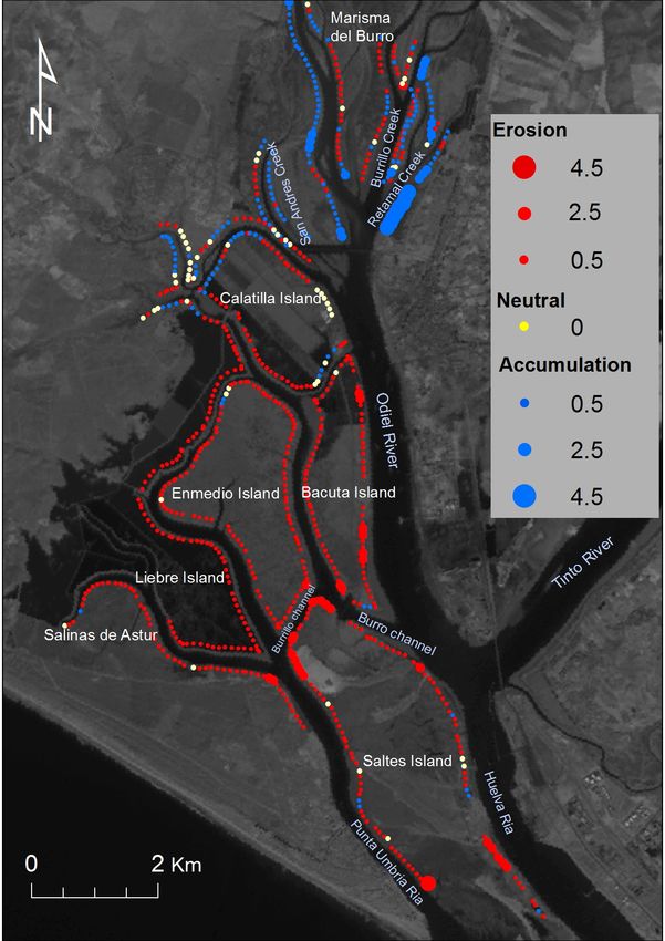
Resources 2019, 8, 50                                                                                   2 of 20

based on semi-empirical models. More recent studies that emphasize ice-sheet contributions to
sea-level rise have estimated that the rise in global mean sea-level could exceed 2 m by 2100 [10,11].
The uncertainty in future sea-level predictions is significant, thus obscuring the magnitude of this
phenomenon and the severity of possible impacts in coastal areas.
      Although there are still uncertainties about future GSLR projections, two things are clear and
certain: (i) that global sea level is rising and (ii) that it varies regionally. With respect to saltmarshes,
Relative Sea-Level Rise (RSLR), which is affected by GSLR and vertical land movements [12], is a
crucial variable for foreseeing potential impacts in specific coastal systems. The saltmarsh net elevation,
and the balance between accretion and RSLR, will determine whether or not a saltmarsh will respond
positively (vertical accretion > sea-level rise) or negatively (vertical accretion < sea-level rise; increasing
the potential for permanent inundation) due to sea-level rise. Future net elevation is difficult to
predict accurately due to complications in saltmarsh processes and responses [13], and uncertainties in
future projections of GSLR and RSLR. Key linkages are non-linear, therefore historical data are only
of limited value and process models are required for future predictions [14] and to assist long term
management strategies.
      Although saltmarshes provide high-value ecological services (such as coastal protection,
food provision and carbon sequestration) [15] and play an important role in coastal ecosystems
and populations, they still remain vulnerable to continued pressures from climate change and
anthropogenic activities [16]. Saltmarshes face the threat of permanent inundation from accelerated
sea-level rise combined with decreasing opportunities for upslope migration due to extensive human
development of coastal areas [1,17]. In this context, those responsible for conservation and management
decisions need appropriate tools with which to gauge the potential impacts of sea-level rise on
saltmarshes and other intertidal ecosystems. However, within this is also the need for sensitivity
and uncertainty analysis in order to evaluate the role of data quality and parameter uncertainties
on predicted response. With this in mind, the aim of this paper is to assess the potential of the sea
level affecting marshes model (SLAMM) [18] for investigating the response of Atlantic-Mediterranean
saltmarshes to future sea-level rise. We also examine its use in managerial schemes, through the
application of sensitivity and uncertainty analysis in the Odiel saltmarshes (Spain, Gulf of Cadiz).
      SLAMM has been widely used in the USA to investigate the potential impacts of sea-level rise
on saltmarshes [19–24]. It has not however been applied to Mediterranean-Atlantic saltmarshes
(as classified by Reference [25] based on the distribution of saltmarsh flora), as found extensively in
South West Europe and North Morocco (Gulf of Cadiz). The vegetation found in southwest Iberian
saltmarshes tends to be different from that found in the Mediterranean basin or in Euro-Siberian
saltmarshes and shows similarities to those found in North-Atlantic Africa. Saltmarsh habitats in the
USA present dissimilarities to those located in SW Europe due to a range of differences in, for example,
extent, vegetation type and structure. For example, saltmarshes in the Gulf of Cadiz comprise complex
creek networks compared with the broad coastal tidal plains of the Atlantic US coast [26]. Despite its
predominant use in the USA, it is still unclear whether SLAMM can be effectively used as a managerial
tool in other parts of the world.

2. Materials and Methods

2.1. Research Design
     The workflow of the approach carried out for this study is shown in Figure 1. This study first
undertakes a sensitivity analysis to explore the relative importance of data quality and resolution in the
elevation data and saltmarsh habitat classification layers. Monitoring and measurement of saltmarsh
habitats are time-consuming and costly, and the acquisition of the SLAMM input layers can require
significant resourcing. Some understanding of where surveying efforts should be focused is therefore
necessary, particularly for authorities with financial constraints. Following this, an uncertainty analysis
was performed on model inputs and different sea-rise scenarios for 2100 was undertaken to identify the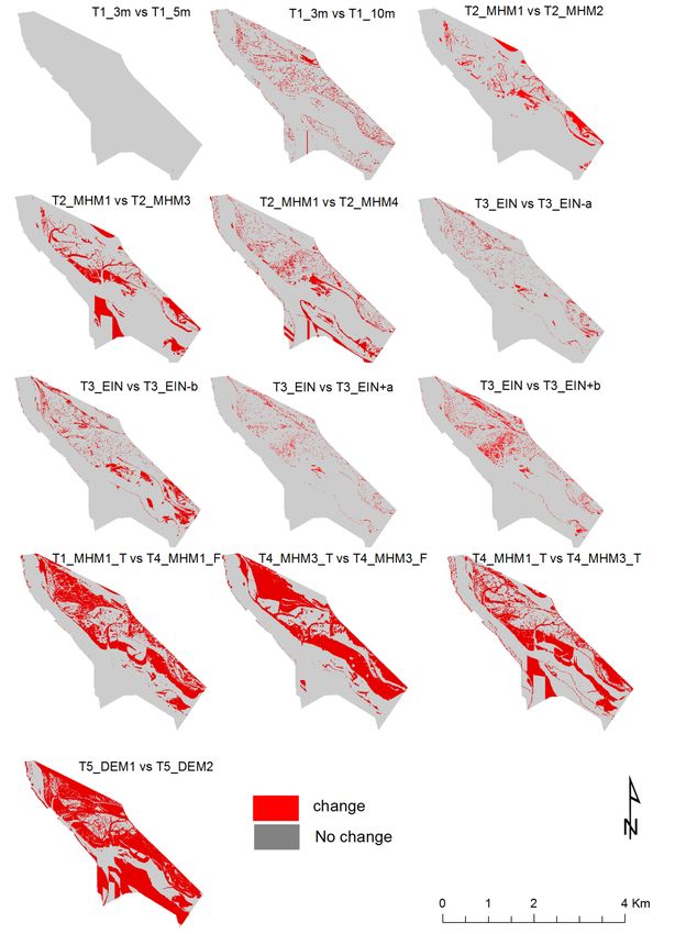
Resources2019,
 Resources  2019,8,8,50
                      x FOR PEER REVIEW                                                                      3 3ofof2120

undertaken to identify the important input parameters that control model output uncertainty and
 important
the chance input    parameters
             of occurrence       that control
                              (taking          model
                                        in account     output
                                                     the      uncertainty
                                                         sea-level           and the chance
                                                                    rise projection           of occurrence
                                                                                      uncertainties          (taking
                                                                                                      for 2100).  To
 in account  the sea-level  rise projection   uncertainties for 2100).  To  that aim,  the best
that aim, the best quality spatial data (selected from the sensitivity analysis) and uncertaintyquality spatial  data
 (selected from
distributions     the sensitivity
                (model              analysis) were
                         input parameters      and uncertainty    distributions
                                                     randomly taken     from these (model  input parameters
                                                                                       distributions  explainedwere
                                                                                                                  in
 randomly   taken   from  these  distributions  explained  in Section  2.5; the  data to generate  the
Section 2.5; the data to generate the distributions were taken from published data in the literature)  distributions
 were
are    taken
    used       from
          to run      published
                   SLAMM     overdata     in theOdiel
                                    the entire   literature) are used
                                                       saltmarshes,      to run
                                                                       where  theSLAMM
                                                                                    potentialover  the entire
                                                                                              saltmarsh        Odiel
                                                                                                          response
 saltmarshes,
due             where
     to sea-level   risethe
                         waspotential
                              assessed.saltmarsh
                                           Finally,response
                                                    erosion due
                                                             ratestoare
                                                                     sea-level  rise waswithin
                                                                        investigated      assessed.
                                                                                                the Finally, erosion
                                                                                                     study area   to
assess the importance of this parameter within the system and their impact on future projections the
 rates are investigated     within  the  study  area  to assess the   importance     of this parameter   within   in
 system and their impactsaltmarshes.
Mediterranean-Atlantic       on future projections in Mediterranean-Atlantic saltmarshes.

                            Figure 1. Workflow of the approach followed for this study.

 2.2. Study Area           Figure 1. Workflow of the approach followed for this study.

       The Area
2.2. Study  Odiel saltmarshes of the Odiel-Tinto estuary (Figure 2) (Gulf of Cadiz, SW-Spain) comprise
 roughly 3000 ha of saltmarshes. The Tinto-Odiel estuary is situated in the central part of the Huelva
      The Odiel saltmarshes of the Odiel-Tinto estuary (Figure 2) (Gulf of Cadiz, SW-Spain) comprise
 coast adjacent to the North Atlantic. Coastal ecosystems here are representative of those found
roughly 3000 ha of saltmarshes. The Tinto-Odiel estuary is situated in the central part of the Huelva
 along the Gulf of Cadiz between Faro (Portugal) and Guadalquivir River (Spain) and North Africa,
coast adjacent to the North Atlantic. Coastal ecosystems here are representative of those found along
 comprising sand spits, large dune systems, barrier islands and tidal inlets, landward of which are
the Gulf of Cadiz between Faro (Portugal) and Guadalquivir River (Spain) and North Africa,
 extensive saltmarshes, lagoons and estuaries that extend far into deeply carved river valleys [27,28].
comprising sand spits, large dune systems, barrier islands and tidal inlets, landward of which are
 The sensitivity analysis to assess spatial model inputs was undertaken on a smaller representative area
extensive saltmarshes, lagoons and estuaries that extend far into deeply carved river valleys [27,28].
 of interest (sub-site shown in Figure 2) around Saltes Island, where habitats such as beaches, tidal flats,
The sensitivity analysis to assess spatial model inputs was undertaken on a smaller representative
 low marsh, high marsh, transitional marsh and up-land are found. Table 1 shows the habitats present
area of interest (sub-site shown in Figure 2) around Saltes Island, where habitats such as beaches,
 and labels used in the SLAMM model habitat map.
tidal flats, low marsh, high marsh, transitional marsh and up-land are found. Table 1 shows the
habitats present and labels used in the SLAMM model habitat map.
Resources 8, 508, x FOR PEER REVIEW
2019,2019,
Resources 4 of 421
of 20
Figure 2. Location of the Odiel saltmarshes and the Tinto-Odiel Estuary (A,B), and location of the
Figure 2. Location of the Odiel saltmarshes and the Tinto-Odiel Estuary (A and B), and location of
sub-site area of interest (C) for testing model sensitivity to spatial inputs.
the sub-site area of interest (C) for testing model sensitivity to spatial inputs.Resources 2019, 8, 50 5 of 20
Table 1. Description of the Odiel saltmarshes habitats with their equivalent SLAMM categories.
SLAMM Category Description
Dry-land Upland (above Highest Astronomical Tide)
Transitional Salt Marsh Estuarine intertidal scrub-shrub
Irreg.Flooded Marsh High saltmarsh
Reg.Flooded Marsh Low saltmarsh
Ocean Flat Marine intertidal unconsolidated shore mud or organic
Tidal Flat Estuarine intertidal unconsolidated shore mud or flat
Estuarine Beach Estuarine intertidal unconsolidated shore sand or beach-bar
Ocean beach Marine intertidal unconsolidated shore sand
Backshore Dry part of an active beach (located above Mean Higher High Water)
Estuarine water Estuarine water
2.3. SLAMM Model
SLAMM version 6.2 (Warren Pinnacle Consulting, Inc., Warren VT, Washington, WA, USA) [29]
was used for this study. This model simulates six key processes/factors involved in wetland
conversions and shoreline modifications during sea-level rise: inundation, accretion, erosion, overwash,
saturation, and salinity. In order to simulate these processes, SLAMM uses spatial data including
digital elevation model (DEM), slope and wetland category maps, and site-specific parameters such as
tidal range or accretion rates. To represent conversion among wetland classes, SLAMM uses a flexible
and complex decision tree incorporating geometric and qualitative relationships [29].
Wetland conversion under sea-level change occurs when sea-level rise exceeds accretion rates and
when the minimum elevation of a cell is below the minimum elevation for a specific wetland category.
The wetland lost fraction (which it is transferred to another category) is calculated as a function of
the cell slope, the minimum elevation for that category, and the lower elevation boundary for that
category [29]. Erosion will occur for those categories adjacent to water when the maximum fetch for a
certain cell is greater than 9 km.
2.4. Sensitivity Analysis of Spatial Model Inputs
A sensitivity analysis was organized to evaluate the role of model input data quality and
resolution, considering both the elevation and habitat inputs. As sensitivity relative to habitat cover
has not been explored previously, the effort here focused on investigating how detail and resolution
in this input layer affect model results (especially for those saltmarshes found in SW Europe, which
are characterized by complex creeks system). However, it should be noted that the presence and
complexity of creek systems vary considerably between marsh systems, so changing the resolution
in spatial inputs has the potential to represent a different type of saltmarsh system. These test runs
were undertaken across a smaller, but a representative region within the Odiel saltmarshes around
Saltes Island (Figure 2). The model inputs tested in this analysis (Table 2) were the marsh habitat
map (MHM) (Figure 3), the digital elevation model (DEM), and the elevation range for each habitat
category. The SLAMM categories used in Figure 3 are described in Table 1, where ‘dry-land’ integrates
‘developed land’ and ‘undeveloped land’. ‘developed land’ refers to upland environments (i.e., built
environments, farmlands) that have been defended against sea-level rise and ‘undeveloped land’ refers
to upland environments that have not been defended. The variation in surface area for each marsh
habitat maps is specified in Figure 4.
Site parameters were kept constant and are summarized in Table 3, and the five sets of tests are
summarized in Table 4. Test 1 explored the impact of cell resolution, and following this, the optimum
(defined as the cell size that optimizes running time without compromising spatial information) cell
size was then used for the remaining tests. Hence, Test 1 with the optimum cell size is used as
the base case, and thus overlaps with the base case for the other tests. Test 2 explores the role of
the marsh habitat map, represented by four different resolutions (MHM_1, MHM_2, MHM_3 and
MHM_4); Test 3 explores the role of habitat elevation range inputs. Test 4 investigates the benefitResources 2019, 8, x FOR PEER REVIEW 6 of 21
Resources 2019, 8, 50 6 of 20
role of the marsh habitat map, represented by four different resolutions (MHM_1, MHM_2, MHM_3
and MHM_4); Test 3 explores the role of habitat elevation range inputs. Test 4 investigates the
of usingof
benefit high-resolution habitat maps
using high-resolution when
habitat mapsonly
when poor resolution
only DEMs are
poor resolution available,
DEMs and here,
are available, the
and
elevation pre-processor tool is also tested. This tool is used when high-quality elevation
here, the elevation pre-processor tool is also tested. This tool is used when high-quality elevationdata are not
available,
data are and
not estimates
available, elevation rangeselevation
and estimates as a function of tide
ranges as ranges and known
a function of tide relationships
ranges and between
known
wetland types and tide ranges (see Reference [29]). Finally, Test 5 explores the differences
relationships between wetland types and tide ranges (see Reference [29]). Finally, Test 5 explores betweenthethe
Lidar-derived DEM and a habitat-corrected Lidar-derived DEM [30].
differences between the Lidar-derived DEM and a habitat-corrected Lidar-derived DEM [30].
Figure 3.3.Marsh
Figure Marshhabitat
habitatmaps
maps(MHM) from
(MHM) Table
from 2 used
Table as different
2 used spatial spatial
as different inputs for testing
inputs for SLAMM.
testing
SLAMM.Resources 2019, 8, x FOR PEER REVIEW 7 of 21
Resources 2019, 8, 50 7 of 20
Figure 4. Variation in surface area (%) for each marsh habitat maps (MHM) from Figure 3.
Figure 4. Variation in surface area (%) for each marsh habitat maps (MHM) from Figure 3.
Table 2. Summary of data used as inputs in SLAMM.
Table 2. Summary of data used as inputs in SLAMM.
Name Description Source
Name Description Source
DEM_1 Unmodified LiDAR-derived DEM (1 m spatial resolution). [31]
DEM_1 Unmodified LiDAR-derived DEM (1 m spatial resolution). [31]
Modified LiDAR-derived DEM (1 m spatial resolution). DEM_1
DEM_2 Modified LiDAR-derived DEM (1 m spatial resolution). [30]
DEM_2 was corrected using a habitat-specific correction factor [30]
DEM_1 was corrected using a habitat-specific correction factor Andalusian Environmental
DEM_3 DEM of the Andalusian Coast (10 m spatial resolution)
Ministry
Andalusian
DEM_3 DEM Habitat
Marsh of the Andalusian
Map derivedCoast (10 m spatial
from supervised resolution)
classification using
MHM_1 Environmental
[31] Ministry
2013 aerial photography and DEM_2 (1 m spatial resolution)
Marsh Habitat Map derived from supervised classification
Manual simplification of MHM1 (5 m spatial resolution) to Derived from MHM1
MHM_2
MHM_1 using 2013remove
aerial small
photography and DEM_2
creeks (retains (1 m spatial
main creeks) (e.g., fewer [31]
small creeks)
Manual simplification resolution)
of MHM2 (5 m spatial resolution) to Derived from MHM2
MHM_3
Manualremove all creeks (only
simplification the main
of MHM1 (5 tidal channels
m spatial remain) to
resolution) (e.g., only thefrom
Derived mainMHM1
channel)
MHM_2 Reclassification of DEM2 based on habitat elevation range. For
MHM_4 remove
Upland smalland
categories creeks (retains
backshore mainthe
(where creeks)
height range (e.g., fewerfrom
Derived small
DEM2creeks)
overlaps, manual editing was carried out) Derived from MHM2
Manual simplification of MHM2 (5 m spatial resolution) to
MHM_3
EIN
Elevation inputs (EINs) per habitat category (zonation) EIN_a (e.g., only
[32]
the main
remove all creeks(± (only theEIN_b
0.2 m); main(tidal
±0.4 m)channels remain)
channel)
Reclassification of DEM2 based on habitat elevation range. For
MHM_4 UplandTable
categories and backshore
3. Site-specific input(where the height
parameters range
required for SLAMM. Derived from DEM2
overlaps, manual editing was carried out)
Input Parameters
Elevation inputs (EINs) per habitat category (zonation) EIN_a
EIN Description Punta Umbría Ria [32]
(±0.2 m); EIN_b (±0.4 m)
Habitat Map Photo Date (YYYY) 2013
Digital Elevation Model Date (YYYY) 2013
Direction Offshore (n, s, e, w) South
Historic Trend (mm/year) 3.3
Mean Tide Level - Vertical datum (m) 0.39
Great Diurnal Tide Range (m) 3.11
Salt Elev. (m above MTL) 2.09
Marsh Erosion (horz. m/year) 0.0105
T.Flat Erosion (horz. m/year) 0.003
Reg. Flood Marsh Accr (mm/year) 6.57
Irreg. Flood Marsh Accr (mm/year) 2.5Resources 2019, 8, 50 8 of 20
Table 4. Summary of the test specifications used for running sensitivity analysis in SLAMM.
Description Test 1 Test 2 Test 3 Test 4 Test 5
Cell size (m) 3, 5, 10 5 5 5 5
Digital Elevation DEM_2 DEM_2 DEM_2 DEM_3 DEM_1
Model DEM_2
Marsh Habitat MHM_1 MHM_1 MHM_1 MHM_1 MHM_1
Map MHM_2 MHM_3
MHM_3
MHM_4
Elev. Prep * False False False False/True False
Elevation ranges EIN EIN EIN EIN EIN
(zonation) EIN_a (±0.2 m)
EIN_b (±0.4 m)
* Elevation pre-processor available in SLAMM.
2.5. Uncertainty Analysis
SLAMM (v-6.2, Warren Pinnacle Consulting, Inc., Warren VT, Washington, WA, USA) has the
ability to perform uncertainty analysis using a Monte-Carlo approach to provide confidence statistics
for model results as a function of input uncertainties. The Monte-Carlo framework implemented the
following steps:
1. Define the input uncertainty distributions
2. Decide how many simulations lead to results which are robust (i.e., not seed sensitive)
and accurate.
3. Automatically generate random input values consistent with the uncertainty distributions.
4. Run SLAMM multiple times with these pseudorandom inputs to evaluate how SLAMM outputs
are affected (full calculation).
5. Analyze the distribution of the model output outcomes to see if there are any common patterns
helping the user to understand the dynamics/interaction of the previously defined uncertainty
distributions of the model inputs.
Uncertainty distributions (step 1) were constructed for each of the model inputs, where it was
assumed that the inputs follow a triangular distribution. Triangular distributions give more importance
to the extreme values that normal distributions, which has been effectively demonstrated in similar
analyses elsewhere (e.g., Reference [33]). It is assumed that the uncertainty distributions of the
accretion rates of both regularly and irregularly flooded marshes follow a joint distribution, but
the other parameters were assumed to be independent of each other. The SLR2100 distribution
values were defined using different published projections for global sea-level rise by 2100 range
between 0.6 and 2.5 m (based on IPCC-scenarios and predictions from References [4,8]); the local
historical sea-level rise trend (Htrend ) used the observed local (Gulf of Cadiz) minimum, maximum
and most likely (average) [34] (source: PSMSL); and the regularly flooded marsh accretion (reg-accre)
and regularly flooded marsh accretion (irreg-accre) used the published Odiel saltmarshes accretion
rates [35]: Minimum (−3 standard deviations of the manifested values), maximum (+3 standard
deviations of the manifested values) and most likely (average of the manifested values).
The next steps were to determine the number of simulations (step 2) and to generate random
inputs (following the uncertainty distributions) for the model (step 3). The number of simulations
(N) for performing uncertainty analysis was determined using Equation (1) (proposed in Sobol’s
method [36]), and used by Reference [33] to perform uncertainty analysis):
N= (k + 2) × M (1)Resources 2019, 8, 50 9 of 20
where k is the number of input factors and M is the sample size (usually between 500 and 1000). In this
analysis, there were four input factors (SLR2100 , Histtrend , reg-accre and irreg-accre) and the value of M
was 1000, leading to a total of 10,000 simulations.
Step 4 following a full calculation approach would require 10,000 simulations using the randomly
generated model inputs to calculate the final output of saltmarsh cover classifications by the year 2100.
Computing time required for this is ~1666 h so an alternative sub-sampling approach was used [31].
Here, a full calculation was performed on a set of input values (~15 values for each parameter, which
means ~60 model runs) covering the range of the uncertainty distribution defined for each input
factors. The outputs obtained using the mentioned set of inputs values were tested and showed a
linear distribution. Thus, the rest of the outputs (9940) were estimated using linear interpolation.
The computing time here was reduced to roughly 6 h, making this approach feasible for this work
using a single computer.
2.6. Erosion Rates
Shoreline erosion and saltmarsh accretion rates were examined throughout the Odiel estuary.
As SLAMM do not take in account erosion values when the fetch is smaller than 9 km, it was important
to investigate the importance and contribution of these values in the system dynamic (marsh loss or
gain). It should be noted that erosion along marsh boundaries can be an important sediment source
for the accreting marsh system (but may favor edge accretion rather than supply to the whole marsh),
and SLAMM do not take in account this process. In this work, erosion rates were determined through
the analysis of shoreline evolution from aerial photographs between 1956 and 2013.
Saltmarsh shorelines were digitized as polylines using ArcGIS v10.2 (Environmental Systems
Research Institute, Redlands, CA, USA); for the years 1956, 1979, 1984, 2001 and 2013 using the
vegetation boundary as the marsh boundary indicator. This indicator was selected due to its stability
over time [37] and due to its unambiguous presence in the aerial imagery. Decadal rates of shoreline
change were derived using the digital shoreline analysis system (DSAS v4.0 (US Geological Survey,
Reston, VA, USA); [38]) at 100 m intervals (782 transects) along the saltmarsh shoreline. DSAS has been
widely used to determine shoreline change in different coastal environments, (e.g., References [39,40]).
The linear regression rate-of-change (LRR), determined by fitting a least squares regression line to all
shoreline points for a particular transect [38] was used here as it expresses a rate of change that takes
into account all time steps across the available data. The LRR statistic was adopted after assessing
different statistic for estimating shoreline rate-of-change in DSAS. For example, endpoint rate (EPR)
statistics (which only uses the initial and final years) masked some inter-decadal variability that was
picked up in the LRR statistic. In the case of weighted linear regression (WLR), although WLR statistics
addresses differences in uncertainties in different shoreline sources, it was not relevant for this study
because there is no significant difference in the accuracy of the surveys (aerial photography).
3. Results
3.1. Sensitivity Analysis Based on Spatial Inputs
The results suggested that the role of elevation is the most important factor in controlling model
outputs. The role of the marsh habitat map is also important; however, it does not have the same
impact on all the defined categories. The spatial model results for the tests performed are compared in
Figure 5. These results are reported by test type and saltmarsh habitat categories.Resources 2019, 8, 50 10 of 20
Resources 2019, 8, x FOR PEER REVIEW 11 of 21
Figure 5. Comparison of the result obtained per test performed. Ti indicates the test carried (e.g., test
Figure 5. Comparison of the result obtained per test performed. Ti indicates the test carried (e.g., test
1, test 2, etc.) followed by the specific input that was modified within each test, where MHM refers
1, test 2, etc.) followed by the specific input that was modified within each test, where MHM refers to
to map habitat map, DEM to the digital elevation model, EIN to elevation inputs and ’3/5/10 m’ to
map habitat map, DEM to the digital elevation model, EIN to elevation inputs and ’3/5/10 m’ to the
the cell size. The pre-processor tool was (by default) off in all the tests, and only in test 4 (T4) was
cell size. The pre-processor tool was (by default) off in all the tests, and only in test 4 (T4) was on
on (stated by ‘T’) and off (stated by ‘F’) to compare the utility of high-resolution habitat maps when
(stated by ‘T’) and off (stated by ‘F’) to compare the utility of high-resolution habitat maps when
high-resolution DEM is not available (see Tables 2 and 4).
high-resolution DEM is not available (see Tables 2 and 4).
With regards to the test type, Test 1 showed that the cell size does not have a great impact in
With regards to the test type, Test 1 showed that the cell size does not have a great impact in
outputs when 3 m and 5 m cell sizes are used. The model outputs slightly varied when a 10 m cell size
outputs when 3 m and 5 m cell sizes are used. The model outputs slightly varied when a 10 m cell
is used (Figure 5), especially for transitional saltmarshes and undeveloped dry land (Figure 5). Thus,
size is used (Figure 5), especially for transitional saltmarshes and undeveloped dry land (Figure 5).
there is a minimal gain in implementing SLAMM with a cell size less than 5 m; SLAMM is flexible
Thus, there is a minimal gain in implementing SLAMM with a cell size less than 5 m; SLAMM is
flexible with regard cell sizes, cell widths usually range between 5 m and 30 m depending on site
and input data availability [29].Resources 2019, 8, 50 11 of 20
with regard cell sizes, cell widths usually range between 5 m and 30 m depending on site and input
data availability [29].
The sensitivity of SLAMM to different habitat maps was evaluated in Test 2; habitat map resolution
considerably influences model results (Figure 6), highlighting the importance of habitat mapping,
especially in open water, estuarine water and saltmarsh categories such as irregularly flooded marsh
and vegetated tidal flat. The impact on the two first categories is due to elevation input ranges for these
categories, which are not defined in SLAMM. Thus, habitat maps strongly control these two categories.
For example, in Figure 6 creeks are evident as only main channels are included in MHM3. Distances
from creeks are used in the accretion sub-model integrated into SLAMM, affecting habitat conversion.
In the case of MHM1 and MHM4, two habitat maps of the same resolution are compared. The results
here showed some differences as well, but these are distributed across the saltmarsh, and along the
margins. The results show that high-resolution habitat maps that represent the complexity of habitats
present (e.g., creeks system) are essential (even when the pre-processor tool is not used), and this has
not been clearly highlighted by other SLAMM users thus far.
Test 3 shows the importance of the habitat elevation range predefined within the model. Variations
of just a few centimeters in the vertical influence the model output and show the importance of correctly
defining the habitat elevation ranges, and also imply that these range inputs should be site specific.
Test 4 shows model output differences when the pre-processor tool is on and off, using a low-resolution
DEM and either the high or low-resolution habitat maps. Results significantly changed when the
pre-processor tool was turned on in both cases. As expected, the model is sensitive to a change in the
resolution of the habitat map when the pre-processor tool is on and a low-resolution DEM is used,
showing important changes when both output results are compared.
Test 5 compares the model results when the LiDAR-derived DEM (DEM1) and modified (using a
habitat-specific correction factor) DEM (DEM2) are used. Results showed that small differences in the
saltmarsh elevation model (Resources
Resources 2019, 8, 50
2019, 8, x FOR PEER REVIEW 1213 of 21
of 20
Figure 6. Surface areas (in hectares) of the outputs for 0.5 m sea level rise projected for 2100 and its
Figure 6. Surface areas (in hectares) of the outputs for 0.5 m sea level rise projected for 2100 and its
variation per category when different inputs are used the optimum test across all categories is Test 1_5
variation per category when different inputs are used the optimum test across all categories is Test
m (which uses the highest resolution input data). * This test out is the same as Test 2_MHM1, Test
1_5 m (which uses the highest resolution input data). * This test out is the same as Test 2_MHM1,
3_EIN and Test 5_DEM2.
Test 3_EIN and Test 5_DEM2.
3.2. Uncertainty Analysis
The uncertainty analysis captured the range of variability of each output (in terms of habitat
surface area). This work is primarily interested in how the ‘total saltmarsh’ fares in the simulations,
thus, for simplicity, the saltmarsh categories have been added together. The ‘total saltmarsh’ is
defined as the combination of regularly flooded marsh, irregularly flooded marsh, and transitional
marsh categories. The uncertainty here is assessed in two ways. The first is based on the uncertaintyResources 2019, 8, 50 13 of 20
3.2. Uncertainty Analysis
The uncertainty analysis captured the range of variability of each output (in terms of habitat
surface area). This work is primarily interested in how the ‘total saltmarsh’ fares in the simulations,
thus, for simplicity, the saltmarsh categories have been added together. The ‘total saltmarsh’ is defined
as Resources
the combination of regularly flooded marsh, irregularly flooded marsh, and transitional marsh
2019, 8, x FOR PEER REVIEW 14 of 21
categories. The uncertainty here is assessed in two ways. The first is based on the uncertainty of the
future
of thesea-level rise by 2100
future sea-level (keeping
rise by the otherthe
2100 (keeping input factors
other inputconstant). The second
factors constant). Theassessment is based
second assessment
on
is based on the uncertainty of the Htrend, reg-accre and irreg-accre input factors for a 1 m by
the uncertainty of the Htrend, reg-accre and irreg-accre input factors for a 1 m sea-level rise 2100.
sea-level
For a given set of 10,000 outputs (obtained using a full calculation with linear
rise by 2100. For a given set of 10,000 outputs (obtained using a full calculation with linear interpolation), the total
saltmarsh changes
interpolation), thewere
totalordered
saltmarshfrom the largest
changes werenegative
orderedtofrom the largest positive,
the largest and the
negative to frequency
the largest
distribution was calculated as shown in Figures 7 and 8.
positive, and the frequency distribution was calculated as shown in Figures 7 and 8.
The
Theeffect
effectofofthe
the1 1mmscenario
scenariosea-level
sea-levelrise
riseusing
usingthe thefull
fullrange
rangevariability
variabilityofofinput
inputfactors
factorswas
was
evaluated
evaluated by analyzing the variability of the outputs. Interestingly, total saltmarsh ashowed
by analyzing the variability of the outputs. Interestingly, total saltmarsh showed bimodala
distribution, with peaks
bimodal distribution, representing
with both negative
peaks representing and positive
both negative change change
and positive (Figure(Figure
7). Overall, 4401
7). Overall,
simulations showed
4401 simulations a decline
showed of the total
a decline of thesaltmarsh, which can
total saltmarsh, be interpreted
which as a 44%aschance
can be interpreted a 44% of this
chance
happening;
of this happening; 214 simulations showed complete elimination of marsh (area relative to the base case (73% probability). However, the highest relative frequency (Figure 8A)
shows that there is a 22% chance of losing between 52% and 66% of the overall saltmarsh when
uncertainty is only based on sea-level rise scenarios. There are 2730 simulations exhibiting an
increase in saltmarsh area (27% probability). The probability of losing saltmarsh is higher when only
sea-level rise8,scenarios
Resources 2019, 50 are considered, highlighting the importance of accretion in the sustainability
14 of 20
of these environments.
Figure 8. Uncertainty analysis for the total saltmarsh considering the full variability of the sea-rise
scenarios defined in the uncertainty distributions, where (A) shows relative frequency of the range of
outputs variability (%), and (B) the cumulative frequency (%).
Relative to the initial case (2013), keeping the site parameters constant, the worst estimate was a
loss of 98% of vegetated saltmarshes by 2100 under a sea-level rise scenario of 2.3 m; the best estimate
was a loss of 91% under a sea-level scenario of 0.6 m. However, when saltmarsh accretion increased
over time, the total saltmarsh loss was reduced leading to the best estimate loss of 7% (under a 1 m
sea-level rise, assuming 3.5 mm year−1 historical sea level trend, 18.5 mm year−1 accretion rates in
regularly flooded marsh and 2.6 mm year−1 in irregularly flooded marsh). These findings demonstrate
once again the importance of future accretion rates (notably sediment availability and supply) in the
fate of the Odiel saltmarshes.
3.3. Assessment of the Erosion Rates
Erosion is also an important factor in saltmarsh loss, and it could exacerbate the impacts of
sea-level rise. However, as it was mentioned previously SLAMM does not take into account erosion
when the fetch is smaller than 9 km. This is the case of the Odiel saltmarshes, and thus erosion was
not considered in the results. In order to assess the importance of this parameter in our study site
erosion rates within the saltmarsh were estimated. Overall, the results showed that erosion is a relevant
parameter and it is essential to model saltmarsh future projections in a context of sea-level rise.
The most striking result in the analysis of saltmarsh shoreline change is the significant difference
in behavior between the northern and southern marshes over recent decades (1956–2013). The Odiel
saltmarshes in the mid/lower estuary have mostly retreated whereas those in the upper estuary have
mostly advanced (Figure 9). Within the upper estuary, the greatest growth is experienced on the east
shore of the Retamal creek, where the horizontal growth rate is >2.5 m year−1 . Saltmarsh shorelines
associated with the islands within the mid/lower estuary show recession over the same time frame:
Enmedio Island, for example, has eroded at a rate of 0.5–2.5 m year−1 .Resources 2019, 8, 50 15 of 20
Resources 2019, 8, x FOR PEER REVIEW 16 of 21
Erosion −1 ) in the Odiel saltmarshes between 1956 and
Figure 9. 9.
Figure Erosionand
andsedimentation
sedimentation rates
rates (in m yyear
(in m −1) in the Odiel saltmarshes between 1956 and 2013
2013 (displayed
(displayed over
over 1987
1987 spot
spot image),
image), estimated
estimated using
using linear
linear regression
regression (LRR);
(LRR); where
where redred dots
dots mean
mean
erosion rates
erosion (retreatment),
rates (retreatment),blue
bluedots
dots sedimentation rates (horizontal
sedimentation rates (horizontalgrowth)
growth)and
andyellow
yellow dots
dots nono
shoreline changes.
shoreline changes.Resources 2019, 8, 50 16 of 20
4. Discussion and Conclusions
SLAMM is an open source model that can be implemented with relative ease. It has been used
to investigate potential impacts of sea-level rise on coastal wetlands in a range of locations, though
primarily the USA [20,21,41–44]. Here, SLAMM was implemented to explore the role of sea-level rise on
Mediterranean-Atlantic saltmarshes using the Odiel system (SW-Spain) as a case study. This has shown
that SLAMM could be used for modelling large expanses of saltmarsh, but results need to be handled
carefully especially when the fetch is smaller than 9 km. An important limitation of SLAMM lies in
its application of lateral erosion, which is not considered when the fetch is smaller than 9 km. This is
an important limitation when modelling Mediterranean-Atlantic saltmarshes, and indeed many of the
infilled estuaries in Europe where the within-estuary open water is usually much narrower than 9 km.
Lateral erosion is an important process when predicting future saltmarsh response due to sea-level
rise, and this rule would need to be modified (as indicated by Reference [45]) when European
saltmarshes are investigated where the fetch will be usually smaller than 9 km. Several authors
(e.g., References [46,47]) have argued that although a saltmarsh may able to accrete vertically in a
context of sea-level rise, lateral erosion due to different factors (anthropogenic and natural) may
significantly impact the pioneer zone, thereby inducing higher saltmarsh loss rates. Although there is
plenty of sediment supply for the Odiel saltmarshes to accrete vertically [31,34], the saltmarsh loss
due to lateral erosion processes is significant and it may induce greater saltmarsh loss in the context
of sea-level rise. The interaction of these factors is not modelled by SLAMM under the mentioned
conditions and it probably underestimates low marsh and pioneer zone loss.
Aside from the lateral erosion issues, SLAMM could be a helpful tool for detecting sensitive
areas within Mediterranean-Atlantic saltmarshes in the context of a rising sea level (e.g., to help to
identify vulnerable zones in combination with field data [24], or to identify where wetland migration
corridors are crucial [48]). For example, model results can help managers and decision makers to plan
adaptation strategies for saltmarshes, and also to define boundaries for further investigation using
more complex physical models (e.g., Reference [49]) or individual-based models (e.g., Reference [50])
that may not feasible when landscape scales are used. However, there are many uncertainties related
to sea-level rise impacts over saltmarshes and it is important to be aware of these when projections are
used to inform saltmarshes and intertidal ecosystem management. The main uncertainties detected
here were due to model limitations and data quality.
The first uncertainty detected in saltmarsh modelling was related to the simplification of the
saltmarsh processes implemented in SLAMM. Models and empirical relationships used to predict
the effects of sea-level rise may simplify relationships (assuming a constant state) [21] and assume
that coastal geomorphology does not change as sea level rises, which is unlikely. SLAMM lacks
feedback mechanisms that may play an important role as sea-level rise accelerates. For example,
increasing inundation of saltmarshes may increase macrophyte production and lead to increased
vertical accretion [51]. Additionally, processes governed by the tidal regime are assumed to be constant
and therefore with increasing progression from the initial condition into a simulation, uncertainties
in model prediction will increase. In this sense, the historical evolution of the studied system
plays an important role in identifying the main drivers acting on the system. By considering past
behavior, the system response due to past sea-level rise, for instance, can provide useful information
for contextualizing the future response of the system. As demonstrated here, uncertainty analysis
considering probability distributions becomes essential to assess the probability of different system
responses. The accurate definition of these probability distributions is crucial to reduce uncertainty,
and historical data should be considered in this process.
The second uncertainty surrounding modelling saltmarsh response to sea-level rise is data source
quality and resolution. The resolution of input data is an important factor in spatial models like
SLAMM and is usually constrained by data source [22]. Elevation data and habitat map accuracy have
been identified here as key components contributing to uncertainty in SLAMM habitat predictions
in the context of sea-level rise. Improving the accuracy of the LiDAR-derived DEMs using saltmarshResources 2019, 8, 50 17 of 20
habitat maps [52] is one approach to reduce elevation quality derived uncertainties. It is highly
recommended to do a rigorous validation of LiDAR-derived DEMs, especially in saltmarshes where
perennial tall vegetation and/or high vegetation density are found. For example, in the case of the
Odiel saltmarshes, the LiDAR-derived DEM showed vertical errors of up to 0.5 m in areas colonized
by Spartina densiflora [30].
Apart from uncertainties related to the model and input data, there are also uncertainties directly
linked to sea-level rise projections; global sea-level rise by 2100 projections range roughly between 0.28
and 1.4 m [3] and could exceed 2 m according to more recent studies [10]. Local projections for the
Odiel saltmarshes estimated from historical trends and future projections using a correlation factor
include 0.64–0.86 m (IPCC scenarios), 1.07–2.27 m [4] and 1.17 m [5,53]. Given the uncertainty in
future sea-level rise, in combination with spatial habitat conversion that may not well reproduced
by predictive models and the site-specific input parameter variability, site-specific projections likely
fluctuate in accuracy [24,54]. Thus, it is essential to consider uncertainty analysis and update the
information based on new research findings when possible.
Finally, management strategies themselves may have uncertain consequences. Robust
management decisions require diverse information, predictions and their associated uncertainty [21].
For this purpose, a multi-criteria decision analysis can provide a suitable tool to integrate different
information [55,56], including results from several models. Apart of combining SLAMM results with
other model outputs in the management strategies, the use of predictive models such as SLAMM could
also be used as a tool for assessing the effectiveness of different management measures for instance.
Thus, the combination of different tools (including uncertainty analysis) could be the key for managing
coastal ecosystems within the uncertain future that they currently face.
Author Contributions: Data curation, M.F.-N. and P.D.-C.; Formal analysis, M.F.-N.; Funding acquisition, J.O.-Z.;
Investigation, M.F.-N. and P.D.-C.; Methodology, M.F.-N. and H.B.; Project administration, J.O.-Z.; Resources,
J.O.-Z.; Supervision, H.B.; Writing—original draft, M.F.-N.; Writing—review & editing, H.B.; P.D.-C. and J.O.-Z.
Funding: This study has been developed within two research projects funded by “Ministerio de Economia y
competitividad (Plan Nacional), grant number CSO2014-51994-P”.
Conflicts of Interest: The authors declare no conflict of interest. The funders had no role in the design of the
study; in the collection, analyses, or interpretation of data; in the writing of the manuscript, or in the decision to
publish the results.
References
1. Smith, S.M. Multi-Decadal Changes in Salt Marshes of Cape Cod, MA: Photographic Analyses of Vegetation
Loss, Species Shifts, and Geomorphic Change. Northeast. Nat. 2009, 16, 183–208. [CrossRef]
2. Nicholls, R.J. Coastal flooding and wetland loss in the 21st century: Changes under the SRES climate and
socio-economic scenarios. Glob. Environ. Chang. 2004, 14, 69–86. [CrossRef]
3. IPCC (Intergovernmental Panel on Climate Change). Climate Change 2014: Synthesis Report. Contribution
of Working Groups I, II and III to the Fifth Assessment Report of the Intergovernmental Panel on Climate Change;
Pachauri, R.K., Meyer, L.A., Eds.; IPCC: Geneva, Switzerland, 2014; p. 151.
4. Pfeffer, W.T.; Harper, J.T.; O’Neel, S. Kinematic constraints on glacier contributions to 21st-century sea-level
rise. Science 2008. [CrossRef] [PubMed]
5. Rahmstorf, S. A semi-empirical approach to projecting future sea-level rise. Science 2007, 315, 368–370.
[CrossRef]
6. Meehl, G.A.; Stocker, T.S.; Collins, W.D.; Friedlingstein, P.; Gaye, A.T.; Gregory, J.M.; Kitoh, A.; Knutti, R.;
Murhy, J.M.; Nosa, A.; et al. (Eds.) Contribution of Working Group I to the Fourth Assessment Report of IPCC on
Climatic Change; Cambridge University Press: Cambridge, UK, 2007; pp. 749–844.
7. Church, J.A.; Clark, P.U.; Cazenave, A.; Gregory, J.M.; Jevrejeva, S.; Levermann, A.; Merrifield, M.A.;
Milne, G.A.; Nerem, R.S.; Nunn, P.D.; et al. Sea level change. In Climate Change, 2013: The Physical Science
Basis; Stocker, T.F., Qin, D., Plattner, G.-K., Tignor, M., Allen, S.K., Boschung, J., Nauels, A., Xia, Y., Bex, V.,
Midgley, P.M., Eds.; Contribution of Working Group I to the Fifth Assessment Report of the Intergovernmental
Panel on Climate Change; Cambridge University Press: Cambridge, UK; New York, NY, USA, 2013.Resources 2019, 8, 50 18 of 20
8. Vermeer, M.; Rahmstorf, S. Global sea level linked to global temperature. Proc. Natl. Acad. Sci. USA 2009,
106, 21527–21532. [CrossRef] [PubMed]
9. Jevrejeva, S.; Moore, J.C.; Grinsted, A. Sea level projections to AD2500 with a new generation of climate
change scenarios. Glob. Planet Chang. 2012, 80–81, 14–20. [CrossRef]
10. DeConto, R.M.; Pollard, D. Contribution of Antarctica to past and future sea-level rise. Nature 2016, 531,
591–597. [CrossRef] [PubMed]
11. Oppenheimer, M.; Alley, R.B. How high will the seas rise? Science 2016, 354, 1375–1377. [CrossRef]
12. Pugh, D.T. Tides, Surges and Mean Sea-Level; John Wiley & Sons Ltd.: New York, NY, USA, 1996.
13. Rybczyk, J.M.; Callaway, C. Surface Elevation Models. In Coastal Wetlands: An Intergrated Ecosystem Approach;
Perillo, G.M.E., Wolanski, E., Cahoon, D.R., Brinson, M.M., Eds.; Elsevier: Amsterdam, The Netherland,
2009; pp. 835–853.
14. French, J. Tidal marsh sedimentation and resilience to environmental change: Exploratory modelling of
tidal, sea-level and sediment supply forcing in predominantly allochthonous systems. Mar. Geol. 2006, 235,
119–136. [CrossRef]
15. Barbier, E.B. Valuing Ecosystem Services for Coastal Wetland Protection and Restoration: Progress and
Challenges. Resources 2013, 2, 213–230. [CrossRef]
16. Hartig, E.K.; Gornitz, V.; Kolker, A.; Mushacke, F.; Fallon, D. Anthropogenic and climate-change impacts on
salt marshes of Jamaica Bay, New York City. Wetlands 2002, 22, 71–89. [CrossRef]
17. Luo, S.; Shao, D.; Long, W.; Liu, Y.; Sun, T.; Cui, B. Assessing ‘coastal squeeze’ of wetlands at the Yellow
River Delta in China: A case study. Ocean Coast. Manag. 2018, 153, 193–202. [CrossRef]
18. Park, R.A.; Manjit, S.T.; Mauseland, P.W.; Howe, R.C. The Effects of Sea Level Rise on US Coastal Wetlands.
The Potential Effects of Global Climate Change on the United States: Appendix B-Sea Level Rise; U.S. Environmental
Protection Agency: Washington, DC, USA, 1989.
19. Clough, J.; Polaczyk, A.; Propato, M. Modeling the potential effects of sea-level rise on the coast of New
York: Integrating mechanistic accretion and stochastic uncertainty. Environ. Model. Softw. 2016, 84, 349–362.
[CrossRef]
20. Hauer, M.E.; Evans, J.M.; Alexander, C.R. Sea-level rise and sub-county population projections in coastal
Georgia. Popul. Environ. 2015, 37, 44–62. [CrossRef]
21. Linhoss, A.C.; Kiker, G.A.; Aiello-Lammensc, M.A.; Chu-Agor, L.; Convertino, M.; Muñoz-Carpena, R.;
Fischere, R.; Linkov, I. Decision analysis for species preservation under sea-level rise. Ecol. Model. 2013, 263,
264–272. [CrossRef]
22. Murdukhayeva, A.; August, P.; Bradley, M.; LaBash, C.; Shaw, N. Assessment of Inundation Risk from Sea
Level Rise and Storm Surge in Northeastern Coastal National Parks. J. Coast. Res. 2013, 29, 1–16. [CrossRef]
23. Sherwood, E.T.; Greening, S. Potential impacts and management implications of climate change on Tampa
Bay estuary critical coastal habitats. Environ. Manag. 2014, 53, 401–415. [CrossRef]
24. Cole Ekberg, M.L.; Raposa, K.B.; Ferguson, W.F.; Ruddock, K.; Burke Watson, E. Development and
Application of a Method to Identify Salt Marsh Vulnerability to Sea Level Rise. Estuar. Coast. 2017,
40, 694–710. [CrossRef]
25. Gehu, J.M.; Rivas-Martinez, S. Classification of European salt plant communities. In Salt Marsh in Europe;
Dijkema, K.S., Ed.; Council of Europe: Strasbourg, France, 1984; pp. 34–40.
26. Orson, R.; Panageotou, W.; Leatherman, S.P. Response of tidal salt marshes of the US Atlantic and Gulf
coasts to rising sea levels. J. Coast. Res. 1985, 1, 29–37. [CrossRef]
27. Ojeda, J. Las Costas Andaluzas. In Geografía de Andalucía; López, A., Ed.; Ariel: Sevilla, España, 2003;
pp. 118–135.
28. Arnaud-Fassetta, G.; Bertrand, F.; Costa, S.; Davidsonc, R. The western lagoon marshes of the Ria Formosa
(Southern Portugal): Sediment-vegetation dynamics, long-term to short-term changes and perspective.
Cont. Shelf Res. 2006, 26, 363–384. [CrossRef]
29. Clough, J.S.; Park, R.A.; Fuller, J. SLAMM 6 Beta Technical Documentation SLAMM 6 Technical
Documentation. 2010; p. 51. Available online: http://warrenpinnacle.com/prof/SLAMM6/SLAMM6_
Technical_Documentation.pdf (accessed on 8 March 2019).
30. Fernandez-Nunez, M.; Burningham, H.; Ojeda, J. Improving accuracy of LiDAR-derived digital terrain
models for saltmarsh management. J. Coast. Conserv. 2017, 21, 209–222. [CrossRef]Resources 2019, 8, 50 19 of 20
31. Fernandez-Nunez, M. Fusion of Airborne LiDAR, Multispectral Imagery and Spatial Modelling for
Understanding Saltmarsh Response to Sea-Level Rise. Ph.D. Thesis, University College London, London,
UK, February 2017.
32. Rubio, J.C.; Figueroa, M.E. Medio Físico, Vegetación de las Marismas de los ríos Odiel y Tinto (Huelva).
Estudios Territoriales 1983, 9, 59–86.
33. Chu-Agor, M.L.; Muñoz-Carpena, R.; Kiker, G.; Emanuelsson, A.; Linkov, I. Exploring vulnerability of coastal
habitats to sea level rise through global sensitivity and uncertainty analyses. Environ. Model. Softw. 2011, 26,
596–604. [CrossRef]
34. Permanent Service for Mean Sea Level (PSMSL). Available online: https://www.psmsl.org/ (accessed on 16
June 2018).
35. Morales, J.A.; Gutiérrez de San Miguel, E.; Borrego, J.E. Tasas de sedimentation reciente en la Ria de Huelva.
Geogaceta 2003, 33, 15–18.
36. Sobol, I.M. Sensitivity estimates for non-linear mathematical models. Math. Model. Comput. Exp. 1993, 4,
407–414.
37. Pajak, M.J.; Leatherman, S.P. The High Water Line as Shoreline Indicator. J. Coast. Res. 2002, 18, 329–337.
38. Himmelstoss, E.A. Dsas 4.0. Instructions Installation Guide User. In Digital Shoreline Analysis System (DSAS)
Version 4.0—An ArcGIS Extension for Calculating Shoreline Change: U.S. Geological Survey Open-File Report
2008-1278; Thieler, E.R., Himmelstoss, E.A., Zichichi, J.L., Ergul, A., Eds.; USGS Numbered Series; U.S.
Geological Survey: Reston, VA, USA, 2009. [CrossRef]
39. Garrote, J.; Díaz-Álvarez, A.; Nganhane, H.V.; Garzón Heydt, G. The Severe 2013–2014 Winter Storms in
the Historical Evolution of Cantabrian (Northern Spain) Beach-Dune Systems. Geosciences 2018, 8, 459.
[CrossRef]
40. Manno, G.; Lo Re, C.; Ciraolo, G. Uncertainties in shoreline position analysis: The role of run-up and tide in
a gentle slope beach. Ocean Sci. 2017, 13, 661–671. [CrossRef]
41. Craft, C.; Clough, J.; Ehman, J.; Joye, S.; Park, R.; Pennings, S.; Guo, H.; Machmuller, M. Forecasting the
effects of accelerated sea-level rise on tidal marsh ecosystem services. Front. Ecol. Environ. 2009, 7, 73–78.
[CrossRef]
42. Akumu, C.E.; Sumith, P.; Baban, S.; Bucher, D. Examining the potential impacts of sea level rise on coastal
wetlands in north-eastern NSW, Australia. J. Coast. Conserv. 2010, 15, 15–22. [CrossRef]
43. Woodland, R.J.; Rowe, C.L.; Henry, F.P.P. Changes in Habitat Availability for Multiple Life Stages
of Diamondback Terrapins (Malaclemys terrapin) in Chesapeake Bay in Response to Sea Level Rise.
Estuar. Coast. 2017, 40, 1502–1515. [CrossRef]
44. Wu, W.; Zhou, Y.; Tian, B. Coastal wetlands facing climate change and anthropogenic activities: A remote
sensing analysis and modelling application. Ocean Coast. Manag. 2017, 138, 1–10. [CrossRef]
45. Pylarinou, A. Impacts of Climate Change on UK Coastal and Estuarine Habitats: A Critical Evaluation of the
Sea Level Affecting Marshes Model (SLAMM). Ph.D. Thesis, University College London, London, UK, 2015.
46. Castillo, J.M.; Luque, C.J.; Castellanos, E.M.; Figueroa, M.E. Causes and consequences of salt-marsh erosion
in an Atlantic estuary in SW Spain. J. Coast. Conserv. 2000, 6, 89–96. [CrossRef]
47. Wolters, M.; Bakker, J.P.; Bertness, M.D.; Jefferies, R.L.; Möller, I. Saltmarsh erosion and restoration in
south-east England: Squeezing the evidence requires realignment. J. Appl. Ecol. 2005, 42, 844–851. [CrossRef]
48. Borchert, S.M.; Osland, M.J.; Enwright, N.M.; Griffith, K. Coastal wetland adaptation to sea level rise:
Quantifying potential for landward migration and coastal squeeze. J. Appl. Ecol. 2018, 55, 2876–2887.
[CrossRef]
49. French, J.R. Numerical Simulation of Vertical Marsh Growth and Adjustment to Accelerated Sea-Level Rise,
Norfolk, U.K. Earth Surf. Proc. Land 1993, 18, 63–81. [CrossRef]
50. Wood, K.A.; Stillman, R.; Goss-Custard, J.D. Co-creation of individual-based models by practitioners and
modellers to inform environmental decision-making. J. Appl. Ecol. 2015, 52, 810–815. [CrossRef]
51. Morris, J.T.; Sundareshwar, P.V.; Nietch, C.T.; Kjerfve, B.; Cahoon, D.R. Responses of coastal wetlands to
rising sea level. Ecology 2002, 83, 2869–2877. [CrossRef]
52. Hladik, C.; Schalles, J.; Alber, M. Salt marsh elevation and habitat mapping using hyperspectral and LIDAR
data. Remote Sens. Environ. 2013, 139, 318–330. [CrossRef]
53. Fraile-Jurado, P.; Fernandez-Diaz, M. Escenarios de subida del nivel medio del mar en los mareógrafos de
las costas peninsulares de España en el año 2100. Estud. Geogr. 2016, 280, 57–79. [CrossRef]You can also read