Commissioning of the instrumentation and launch of the scientific exploitation of OARPAF, the Regional Astronomical Observatory of the Antola Park
←
→
Page content transcription
If your browser does not render page correctly, please read the page content below
Commissioning of the instrumentation and launch of the scientific
                                               exploitation of OARPAF, the Regional Astronomical Observatory of
                                               the Antola Park

                                               Ricci D.a , Tosi S.b, c , Cabona L.d , Righi C.d , La Camera A.e,* , Marini A.b , Domi A.b,c ,
                                               Santostefano M.b , Balbi E.f , Nicolosi F.b , Ancona M.e , Boccacci P.e , Bracco G.b,g ,
                                               Cardinale R.b,c , Dellacasa A.e,** , Landoni M.d , Pallavicini M.b,c , Petrolini A.b,c , Schiavi C.b,c ,
                                               Zappatore S.h , Zerbi F. M.d
                                               a
                                                 INAF-Osservatorio Astronomico di Padova, Vicolo dell’Osservatorio 5, 35122 Padova, Italy.
                                               b
                                                 Università degli Studi di Genova, DIFI Dipartimento di Fisica, Via Dodecaneso 33, 16146, Genova, Italy.
                                               c
                                                 INFN-Sezione di Genova, Via Dodecaneso 33, 16146 Genova, Italy.
                                               d
                                                 INAF-Osservatorio Astronomico di Brera, Via E. Bianchi 46, 23807, Merate (LC), Italy.
arXiv:2011.13262v1 [astro-ph.IM] 26 Nov 2020

                                               e
                                                 Università degli Studi di Genova, DIBRIS Dipartimento di Informatica, Bioingegneria, Robotica e Ingegneria dei
                                               Sistemi, Via all’Opera Pia 13, 16145, Genova, Italy.
                                               f
                                                 Università degli Studi di Genova, DISTAV Dipartimento di Scienze della Terra, dell’Ambiente e della Vita, Corso
                                               Europa 26, 16132, Genova, Italy.
                                               g
                                                 CNR-Area della Ricerca di Genova, Via De Marini 6, 16149 Genova, Italy.
                                               h
                                                 Università di Genova, DITEN Dipartimento di Ingegneria delle Telecomunicazioni, Elettrica, Elettronica e Navale,
                                               Via all’Opera Pia 11A, 16145, Genova, Italy.
                                               *
                                                 Now at Teiga Srls, Viale Brigate Partigiane 16, 16129, Genova, Italy.
                                               **
                                                  Now at Drafinsub Srl, Via al Molo Giano, 16128, Genova, Italy.

                                               Abstract. The OARPAF telescope is an 80cm diameter optical telescope installed in the Antola Mount Regional Re-
                                               serve, on the Ligurian Apennines in Northern Italy. We present the the improvements and interventions that have been
                                               implemented since the inauguration. The characterization of the site has resulted in a typical background brightness
                                               of 22.40mAB (B filter) – 21.14mAB (I) per arcsecond squared, and a 1.5–3.000 seeing. An estimate of the magnitude
                                               zero points for photometry is also reported. The material under commissioning foresees 3 CCD detectors for which
                                               we give the linearity range, gain, and dark current; a 31 orders échelle spectrograph with R ∼ 8500–15000, and a
                                               dispersion of n = 1.39 × 10⁻⁶ λ + 1.45 × 10⁻⁴ , allowing radial velocity measurements up to 15.8km/s; and a long slit
                                               spectrograph currently under commissioning. The scientific and outreach potential of the facility is proven in different
                                               science cases, such as exoplanetary transits and AGNs variability. The determination of time delays of gravitationally
                                               lensed quasars, and the tracking and the study of asteroids are also discussed as prospective science cases.

                                               Keywords: telescopes, photometry, spectroscopy, echelle spectroscopy, commissioning.

                                               Corresponding author: Davide Ricci, davide.ricci@inaf.it

                                               1 Introduction
                                               The Regional Astronomical Observatory of the Antola Park (OARPAF), located at 44°350 28.4600 N,
                                               9°120 12.4900 E, in the territory of Comune di Fasciaa , is a facility situated in the Ligurian Apennines
                                               at an altitude of about 1 480m above sea level. The altitude, together with the extremely small light
                                               pollution distinctive of the area, has promoted the set up of an 80cm, f /8 Cassegrain-Nasmyth
                                               alt-azimuthal optical telescope, inaugurated in 2011, which is one of the few and one of the largest
                                               optical telescopes in Italy available in a public facility.1 It also features a fully equipped conference
                                               room, a planetarium, a library and guest rooms for scientists.
                                                   a
                                                       https://goo.gl/maps/upEY3

                                                                                                          1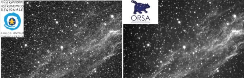
The telescope was initially equipped with a set of scientific instruments, including a SBIG
STL 11000 M camera with an embedded filter wheel with standard Johnson-Cousins U BV RI
photometric filters, and a FLECHAS échelle, optical fiber spectrograph with a ATIK Monochrome
11000 M.
    The University of Genoa (Italy), took charge of scientific operations by virtue of an agreement
with the Antola Natural Reserve, who manages the facility on behalf of Comune di Fascia. An
interdepartmental center was created to group researchers of the University of Genoa interested
in astronomy and in the related instruments and technology. The center, named ORSAb , standing
for Observations and Research in the Science of Astronomy, groups together researchers from the
Department of Physics (DIFI), the Department of Mathematics (DIMA), the Department of Chem-
istry and Industrial Chemistry (DCCI), the Department of Informatics, Bioengineering, Robotics
and System Engineering (DIBRIS) and the Department of Telecommunications, Electric, Elec-
tronic and Naval Engineering (DITEN). Scientific collaborations have been established with the
National Institute for Astrophysics (INAF) and the National Institute for Nuclear Physics (INFN).
Preliminary results and the scientific potential of the facility are encouraging.2, 3 Indeed in 2017,
DIFI participated in the call by the Italian Ministry for Education, University and Research (MIUR)
named “Departments of Excellence”, by presenting a project aimed at launching new research lines
in astrophysics, as well as an augmented didactic offer in the field. OARPAF played an important
role in the project both for its scientific usage and for its adequacy to form new students in the field
of observational optical astronomy. The project was indeed financedc , allowing to contribute to its
scientific progresses and full remotization.
    In particular, the instrumentation was improved by the purchase of a LHIRES III spectrograph,
a Class-1 CCD SBIG STX 16801 camera, a FW 7- STX filter wheel with standard, 50mm U BV RI
and Hα filters.
    After briefly introduce the remote control strategy (Sect. 2), we firstly describe the steps un-
dertook for the site characterization as well as the calibration and commissioning of the OARPAF
instrumentation (Sect. 3), with the goal of using it for scientific purposes. Consequently, we intro-
duce astrophysical projects achievable with the facility, some of which have resulted in scientific
publications (Sect. 4). Finally, we address its relevance for didactic and outreach events (Sect. 5).
A summary of results, as long as conclusions, are shown in Sect. 6.

2 Remote control
Initially, the facility and the dome of the telescope were conceived to be operated only locally and
manually. Consequently, the scientific usage of the telescope was limited. Of course, being able to
remotely control the dome and the other instruments represents a huge advantage for the scientific
exploitation of the telescope. Therefore, with the goal of remotely controlling it, we implemented a
first modification towards an automated use of the dome by developing a Python script running on a
Raspberry-PI to query the control center for position, and interacting with the dome by an Arduino
platform. The necessary works to remotely control the dome started immediately, and the needed
set of instruments was bought: these include a new weather station with pluviometer, anemometer,
hygrometer and thermometer, an all-sky camera, two IP webcams, and a new electronic system
with an encoder directly interfaced to the interlock system.
   b
       http://www.orsa.unige.net/index.php/en/about/
   c
       https://www.anvur.it/attivita/dipartimenti/

                                                   2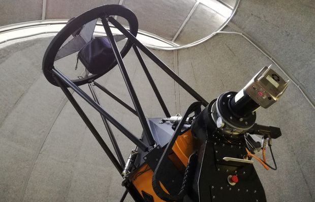
This way, remote operators can monitor the weather and sky conditions at OARPAF and the
possible presence of visitors; for the safety of the telescope, the dome will automatically close
in case of bad weather and in case of prolonged absence of the Internet connection. A custom
software framework under the Linux operating system was designed to manage all the parts.
    During the first years, the original dome showed problems of water leakage, posing a serious
risk of damaging the telescope: therefore, a new dome was installed in 2020 by the Gambato
companyd .
    Since remote operations must be fully reliable, a stable access to the Internet is mandatory.
Unfortunately, the access link currently in use at OARPAF does not yet satisfy the necessary re-
quirements of stability. Several actions for improving the overall quality-of-service and the service
level agreements of the Internet connection are planned for the end of 2020 by the Liguria Digi-
tale companye . In the near future, the remote control of the facility will be obtained in two ways,
described hereafter.

2.1 Ricerca
To date, a full remote control is not yet available. The newly installed dome was provided with
a commercial control software, named Ricerca, developed by OmegaLabf , operating under Win-
dows. Ricerca makes use of ASCOM drivers and can be used together with the telescope software
to remotely manage the observatory, its monitoring systems, the dome, and the detectors. The
software interfaces with a hardware module called OCSIII, provided with relay control switches
for the several mentioned subsystems, also including dome light for flat fields.

2.2 Web interface
To allow more flexibility in the framework of future development, a completely Linux-based cus-
tom control software is being set up. The latter uses top modern internet technologies to operate
through commands given via a web browser, or script, through a web Application Programming
Interfaces (API). The interface implements the html and javascript languages via the popular Boot-
strap 4 framework, while the V8-based technology node.js and mongodb are used for the
server side development and storing purposes.4 It already allows the control of the SBIG cameras
and the all-sky camera as a test benchmark and it will be implemented in order to monitor and
control the dome and the telescope, as well as the weather station and the webcams, producing
real-time images.
    Moreover, it will allow to control and schedule public visits and scientific operations. In addi-
tion, it will be easily usable by schools for public events and outreach activities.

3 Site characterization and commissioning of the telescope and the instruments
To allow for scientific measurements and to verify the feasibility of new ideas, it is important to
characterise the site and the instruments. The main measurements and calibrations that have been
performed include:

       • Extended pointing model, with a large number of standard stars;
   d
     https://www.gambato.it/
   e
     https://www.liguriadigitale.it/
   f
     http://atcr.altervista.org/ita/index.html

                                                  3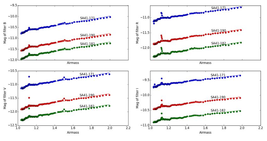
Fig 1: The OARPAF telescope with the SBIG STL 11000 M camera on the derotated Nasmyth focus.

       • Determination of the typical seeing of the site;

       • Measurement of the dark current of the CCDs;

       • Determination of the quantum efficiency of the CCDs;

       • Determination of the efficiency of the photometric filters.

       • Determination of the sensitivity of the échelle spectrograph;

Using the above mentioned information, an Exposure Time Calculator (ETC) has been written to
be able to determine the needed exposure time to observe a given target depending on the desired
signal-to-noise ratio, considering the photon flux of the source, all attenuation and distortion factors
and all background sources. A data analysis pipeline has been written to obtain a fully calibrated
and background subtracted image starting from the raw data.

3.1 Telescope
The OARPAF telescope (Fig. 1) is a 0.8 m alt-azimuthal Cassegrain-Nasmyth T0800-01 telescope
manufactured by ASTELCO Systemsg . With an alt-azimuthal mount, the image of the sky ro-
tates in the focal plane during the time of data acquisition then a derotator is used to capture
long-exposure images. The optical scheme comprises a primary concave parabolic mirror with a
diameter of 0.8m, is made of Schott Zerodur 85mm height coated with Al+MgF2 with reflectivity
greater than 95%, that reflects light towards a secondary convex hyperbolic mirror; a comparatively
small tertiary flat mirror reflects the light to one of the 2 Nasmyth foci of the telescope at f /8, with
a focal length of 6.4m.
    In fact, a peculiarity of OARPAF consists in the tertiary flat mirror, that can be manually rotated
to switch the Nasmyth focus between
   g
       http://www.astelco.com

                                                    4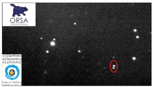
STL                                     Atik                            STX
         70000

         60000

         50000

         40000
Counts

         30000

         20000

         10000

             0
              0.0   0.5   1.0   1.5     2.0    2.5   3.0   0   1             2         3   0   2      4        6       8   10
                           Exposure time (s)                       Exposure time (s)               Exposure time (s)
Fig 2: Linearity test of the SBIG STL 11000 M camera, the ATIK Monochrome 11000 M, and the
SBIG STX 16801 camera at -10°C, +1°C, and -20°C, respectively. Results of a linear fit are
superimposed to the data points. Empty dots have been sigma-clipped. All cameras are linear in
the approximate range 4 000–60 000 counts.

            • the “observing flange”, for outreach usage, provided a with a manual focuser and a set of
              oculars;

            • the “scientific flange”, where the derotator is placed. The scientific flange includes a field
              flattener, in order to flatten the focal plane so that not only the central point but the whole
              image appears fully focused. Up to now, we used the SBIG STL 11000 M camera on this
              flange, and we measure a plate scale of 0.2900 /px.

3.2 Pointing model
Accurate pointing or positioning of a telescope is of paramount importance for any telescopic sys-
tem in order to be productive. The telescope has various static and dynamic pointing errors: these
must be compensated with the help of position measurements of reference stars. The A S T EL OS
software provided by Astelco Systems allows users to make a new pointing model or improve an
existing one by adding more measurements. The software algorithm comprises 25 coefficients,
that are calculated by measuring the offset between the instrumental position of an object and its
calculated theoretical position. The pointing velocity of the telescope can reach 20°/s, and the
acceleration 20°/s2 . After refining our pointing model, we reached a pointing accuracy is < 1000
root mean square, and a tracking accuracy of < 100 per 30 minutes.

3.3 Detectors and filters
 OARPAF originally had two CCDs:     a SBIG STL 11000 M camera and a ATIK Monochrome 11000 M.
Both use a Kodak KAI -11000 sensor with 11 million 9µm2 pixels, covering 36×24.7mm. In 2019,
a new SBIG STX 16801 camera with a Class-1 CCD has been added. This camera uses a Kodak
KAF -16801 sensor with 16 million 9µm2 pixels, covering 36.8 × 36.8mm. All three CCDs can be
cooled at least −30°C below ambient temperature.
    The quantum efficiency of the CCDs, defined as the ratio between incoming photons to con-
verted electrons, varies with the wavelength, having a maximum of around 50% at 500nm.
    The photometric filters are a set of standard U BV RI Johnson-Cousins filters,5 centered around
the wavelengths 360 (U ), 420 (B), 550 (V ), 640 (R) and 790 (I) nm, respectively, with a full width
at half maximum (FWHM) bandwidth of 60, 90, 85, 140 and 150 nm, respectively.

                                                                     5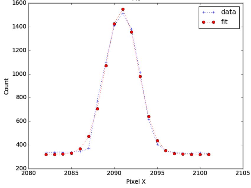
Fig 3: The telescope and a sample image of the Vela Nebula (before and after debiasing and flat-
fielding used for outreach purposes.

     The existence of a linear relation between the charge collected within each pixel and the dig-
ital number stored in the output image has been verified with exposures of various duration on a
uniform and constant light source: a linear relation holds up to very high counts, where a deviation
from linearity is seen. Fig. 2 shows the counts in ADU as a function of the exposure time for the
three CCDs. We found a good linearity range for all detectors (4 000-60 000 counts) with a gain
G of 1.040e− /ADU for the SBIG STL 11000 M camera, 0.996e− /ADU for the ATIK Monochrome
11000 M, and 0.998e− /ADU for the SBIG STX 16801 camera. The dark current D was determined
by means of sets of 60min exposure dark frames. We obtain: 0.70ADU/px/s for the SBIG STL
11000 M camera at −10°C, 0.94ADU/px/s for the ATIK Monochrome 11000 M, at −3°C, and
0.28ADU/px/s for the SBIG STX 16801 camera at −20°C.
     Having now three CCDs, we plan to use them as follows:

    • The new SBIG STX 16801 camera will be dedicated to high-performance photometry, re-
      placing the SBIG STL 11000 M camera which has been used until now;

    • The SBIG STL 11000 M camera will be used with the new LHIRES III spectrograph;

    • The ATIK Monochrome 11000 M is used in conjunction with the FLECHAS spectrograph.

3.4 Data reduction
The calibration procedure is mainly intended to remove additive contributions to the background,
such as the electronic pedestal level, the dark current, the multiplicative gain and illumination
variations across the chip. The goal of the data reduction pipeline is to minimize the contribution
of deterministic factors in the uncertainties and, at the same time, by preserving information about
the noise sources, so that users can evaluate the random uncertainties of the reduced data. The
raw counts of a pixel in position x, y in a CCD frame can be calculated as s(x, y) = B(x, y) +
tD(x, y) + tG(x, y)I(x, y) + N , where B(x, y) is the bias value of each pixel, t is the integration
time, D(x, y) is the dark current, G(x, y) is the sensitivity gain and I(x, y) is the light flux reaching
the pixel, while N is any other irreducible noise source of the pixels. B, D and G are measured
from bias, dark and flat frames, respectively.
    Bias frames measure the readout noise and correspond to observations without exposure to
light (shutter closed), for a total integration time of 0 seconds: several frames are taken so that a

                                                   6
median can be determined with reduced statistical uncertainty. If we allow the CCD to integrate
for some amount of time, without any light falling on it, there will be a signal caused by thermal
excitation of electrons in the CCD: this is called dark signal and it is very sensitive to temperature.
All CCDs have non-uniformities, that is, a uniform illumination of the CCD does not yield
an equal signal in each pixel (even ignoring noise). Small scale (pixel to pixel) non-uniformities
(typically a few percent from one pixel to the next) are caused by slight differences in pixel sizes.
Larger scale (over large fractions of the chip) non uniformities are caused by various effects, such
as small variations in the silicon thickness across the chip, non-uniform illumination caused by
telescope optics (vignetting). These can sum up to variations of around 10% over the chip. To
measure and correct for these non-uniformities, the entire CCD is illuminated by a uniform source
of light and flat field data are taken. At OARPAF, the twilight method6 has been applied until the
new dome was equipped with a board to take dome flat fields.
A Python pipeline has been developed to remove the various background sources and derive a
calibrated image, as shown in Fig. 3. The development of the pipeline also foresees field solving by
querying astrometry.net, and matching sources from the GAIA DR2 catalog7, 8 in order to
perform automatic aperture photometry. Field solving also overcomes errors due to the possibility
of low tracking accuracy, especially on derotation. If this happens, light from a given object will
not populate the same pixel for each frame. Further implementation foresees the use of a separate,
on-axis guiding camera and the tip-tilt lens corrector in order to correct the pointing during frame
acquisition.
3.5 Average sky background
The largest contribution to the sky emission comes from the moonlight, which is particularly strong
in the near UV and decreases towards larger wavelengths becoming negligible in the near IR. Of
course, the scattered moonlight depends strongly on the moon phase and changes the sky brightness
by huge factors, up to 30 in the visible band. We used the SBIG STL 11000 M camera at OARPAF
to measure a typical sky brightness during a new moon phase. We find a value of of 22.40 mAB /00 2
in the B filter, down to 21.14 mAB /00 2 in the I filter.
3.6 Seeing
The distortion induced by the atmosphere is expressed by the seeing parameter. An estimate of
the typical seeing at the OARPAF site was measured by determining the point spread functions
of several stars, assumed to be point sources, and fitting with 2-dimensional Gaussian functions.
The seeing is the average Full Width at Half Maximum (FWHM). During a typical summer night,
when the seeing is expected to be the worst because of larger humidity, we find at OARPAF using
the SBIG STL 11000 M camera a seeing of 2.500 , with a general range of variability of between 1.500
and and 3.000 .
3.7 Photometric calibration
When an image is taken, the conversion factor from counts to scientific units is not known a pri-
ori, and a photometric calibration of all instruments is mandatory.9, 10 In this respect, a series of
standard stars, whose light output in various passbands of photometric systems has been carefully
measured and selected by the TOPCAT program,11 are used. The stars are observed at their maxi-
mum elevation in the sky, typically at an air mass value (AM ) smaller than 1.15. The instrumental
7Fig 4: Magnitude as a function of the air mass in various filters for three reference stars.
zero points are determined as a function of the color index in different passband filters. The cal-
ibrated magnitude Mλ1 at a defined passband centered around the wavelength λ1 is the sum of
more components: Mλ1 = zλ1 + mλ1 − kλ1 AM + cλ1 (mλ1 − mλ2 ), where zλ1 is the zero point
of the photometric system at a defined passband, mλ1 is the instrumental magnitude, kλ1 is the
atmospheric extinction coefficient, AM is the air mass at the observation time, cλ1 is a color term
and the difference mλ1 − mλ2 is the instrumental color index from two different filters. In fact,
the atmospheric extinction is a complex phenomenon to model because many effects are involved;
it is more prominent in the U , B and V filters, while it is much smaller in the R and I filters. At
first approximation, the extinction has a first order term proportional to the air mass at the time of
observation, which takes into account the attenuation due to the mass of air traversed by photons,
and a second order term, which takes into account its influence on the color variation. At the effec-
tive wavelength λ, the instrumental magnitude m is related to the extra-atmosphere instrumental
magnitude m0 by Bouguer’s law m = m0 + kλ AM , where kλ is the extinction coefficient (mea-
sured in mag/AM ). A fit of observed magnitudes of standard stars at different air masses allowed
to determine the extinction coefficients for every filter.
Results of extinction coefficient at OARPAF, calculated using the SBIG STL 11000 M camera
and the related filters, are shown in Table 1a and Fig. 4. Once these have been determined, the zero
points and the color terms can be in turn measured. We report the results in Table 1b. We verified
the goodness of the determination of the zero points and color terms by comparing the theoretical
expected magnitudes with the Mλ calculated magnitudes for various known sources.
3.8 The FLECHAS spectrograph
OARPAF is equipped with FLECHAS , a Fiber-Linked ECHelle Astronomical Spectrograph:12 it is an
échelle sectrograph specifically designed for class 1m telescopes with focal ratios of f /8 to f /12
by the Astelco Systems company. The optical design is optimized for seeing conditions of around
8Fig 5: FLECHAS spectrum taken with the ATIK Monochrome 11000 M.
1.500 and for typical pixel sizes of most common CCDs. The expected seeing spot size determines a
pin hole size of around 150µm, and in turn yields an effective resolving power between R ∼ 8500,
and R ∼ 15000 with an image slicer to suppress scintillation effects; here R is defined as the ratio
λ/∆λ between a given wavelength λ and the minimum resolvable wavelength difference ∆λ.
We paired the FLECHAS with the ATIK Monochrome 11000 M. The wavelength range of the
optics of the spectrograph is 350–850nm, with a transmission coefficient of 80%. We measured
the stability of FLECHAS using an embedded Thorium-Argon (ThAr) calibration source, and we
find to be 0.46px, at 95% confidence level over one hour.
The FLECHAS equipped with the ATIK Monochrome 11000 M covers 31 échelle orders, as seen
in Fig. 5. We measured a variable order separation from 4px to 105px. All orders measure about
30px in height, exhibiting a double peak profile because of the image slicer (see Fig. 6).
The calibration in wavelength and the dispersion are obtained again using the ThAr lamp. The
dispersion n increases with wavelength with a linear relation of the form: n(nm/px) = aλ(nm)+b.
λ1 (λ2 ) Zero point Color term
Passband filter Extinction coefficient B (V) 23.03 ± 0.06 −0.26 ± 0.12
B 0.742 ± 0.005 V (B) 22.72 ± 0.03 0.04 ± 0.06
V 0.543 ± 0.002 V (R) 22.73 ± 0.02 0.14 ± 0.13
R 0.463 ± 0.005 R (V) 22.40 ± 0.04 0.60 ± 0.40
I 0.376 ± 0.005 R (I) 22.63 ± 0.25 0.15 ± 0.19
(a) Measured extinction coefficients for each pass- I (R) 21.93 ± 0.40 0.90 ± 0.30
band filter. (b) Zero points and color term.
Table 1: SBIG STL 11000 M camera filter parameters. Color terms determined for wavelength λ1
at the nominal central value of each filter, with respect to a λ2 at the value of a nearby filter.
9Fig 6: Trend of the counts in the cross direction to the dispersion for the 31 orders of the FLECHAS.
(a) An example of Gaussian fit (red dots) to a ThAr (b) Resolving power R as a function of the wavelength
peak data (blue crosses): the FWHM of this peak is (red). The blue (green) lines use the median (mean)
found to be 4.46px. FWHM.
Fig 7: Example of ThAr peak data and resolving power of the FLECHAS.
We find a and b to be 1.39 × 10⁻⁶ nm/px and 1.45 × 10⁻⁴ nm/px, respectively.
The spectral resolving power of FLECHAS as a function of the λ has been determined by a
Gaussian fit to the peak along the direction of dispersion (see Fig. 7a), in order to measure the
FWHM of the emission lines detected in the ThAr calibration spectra, and averaging the FWHM
over the various orders (Fig. 7b). Such measured resolving power allows us to establish that the
minimum appreciable radial velocity of a star is around 15.8km/s.
3.9 The LHIRES III spectrograph
In 2019, a Shelyak LHIRES III medium-resolution was purchased. This is a long-slit spectrograph
with slit width of 25µm, 1200 lines per mmgrism and a resolving power of R ∼ 5800.
We decided to pair the LHIRES III to the SBIG STL 11000 M camera. In this configuration, and
basing on the producer documentation, we estimate at OARPAF a maximum observable magnitude
of mV ≈ 10, for a signal-to-noise ratio of 100 and 1 hour exposure. We also calculate a mean
sampling is about 0.034nm/px, which in turn yields a mean field width of one acquisition4 of
≈ 138nm. A micro-metric screw allows the shift of the central wavelength, so that most of the
10TrES-3b combined light curves and fit TrES-3b relative radius
V Exofast fix.Kund. TAP fix.Turner
1
V
R
filter
0.99 R
normalized flux
Rc
I literature
0.98 Rc
0.155 0.165 0.175 0.185
0.97 I Rp/R*
0.96
TrES-3b Mid-times
0.0021
0.95 UDEM
0.0014
KPNO
0.0007
O-C [d]
StPr
0 0
residuals
TCS
-0.0007
-0.02 OARPAF
-0.0014
SPM
-0.04 -0.0021
-0.05 0 0.05 4000 5000 6000 7000 8000 9000
Phase Time to Tmid - 2450000 [d]
Fig 8: TrES-3b recent results3 obtained with OARPAF contribution (red marks). Left: Light
curves fitting and residuals. Up: Ratio between TrES-3b and host star radii obtained with dif-
ferent procedures (EXOFAST and TAP modelling), compared with values found in the literature
(grey). Down: Observed-Calculated Mid-Time transits vs Mid-times.
≈ 300nm wavelength range of the SBIG STL 11000 M camera can be in principle covered with two
exposures. The Shelyak spectrograph has not been fully commissioned yet: its calibration and first
usage will be presented in a different publication.
4 Science cases
The scientific reach of OARPAF is wide. Observations and preliminary results obtained during
the past years illustrate the large potential of the facility: these include either observations for
which small, 1m class, telescopes, such as OARPAF, have enough sensitivity to be competitive,
and measurements that require long campaigns, typically not possible with big telescopes, whose
observation time has to be shared between many projects.
The scientific potential of the telescope has been presented in several nationalh and international
conferences2, 4, 13, 14 and in master-degree theses of students of the University of Genova.15–17
In the followinw subsections we present such results and future prospects.
4.1 Exoplanetary transits
Planets orbiting stars other than the Sun have been first discovered in the 90s and along the years
their number increased and passed 4000i . They can be detected using different experimental meth-
ods. For OARPAF, the photometric transit18 is the most suitable method. To measure the needed
light curves, we made use of defocused photometry19 allowing the star hosting the target exoplanet
h
http://events.iasfbo.inaf.it/gloria/od_programme.php
i
http://exoplanet.eu
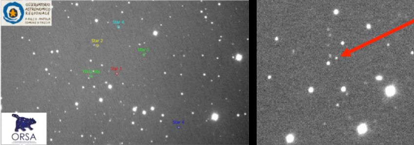
11Fig 9: Left: The field of view showing the faint quasar SDSS J223827.17+135432.6 (labelled
WLQ-obj in green) and 5 reference stars for differential photometry. Right: a zoom around the
quasar, indicated by a red arrow.
to cover many pixels, and to obtain magnitude dispersion levels comparable to those of space tele-
scopes. The measurements thus obtained are practically unaffected by any instrumental defects,
by calibration biases and by variations of the quality of the observing night, an important aspect
for measurements that can last several hours.
At OARPAF, we observed, with the SBIG STL 11000 M camera, the exoplanet TrES-3b using
the defocused photometry technique. The observation contributed to a peer review publication,3
where data taken also at the Observatorio Astronomico Nacional de San Pedro Martir (Mexico),
Observatorio de la Universidad de Monterrey (Mexico) and Telescopio Carlos Sanchez at the Ob-
servatorio del Teide (Spain) were combined (Fig. 8), allowing to derive physical and orbital pa-
rameters of the planet. Other exoplanets that we observed include WASP-58b, HAT-P-3b and
HAT-P-12b,13, 16 and the data reduction is ongoing using the pipeline described in Sect. 3.4.
4.2 Active galactic nuclei
Active galactic nuclei are the most luminous persistent sources of electromagnetic radiation. Some
of them display jets of relativistic particles and are named blazars when the jet points to the ob-
server. It is possible to distinguish among various models for blazars by measuring the optical
variability with long monitoring campaigns12, 20–23 . A feasibility test of such measurements has
been done in order to make sure that such sources can be observed at OARPAF. Considering all the
characteristics of the telescope, the instruments and the site, several observable blazars have been
identified.
A very faint object, SDSS J223827.17+135432.6, with magnitude mR = 20 in the R
filter, could be observed (Fig. 9) with a large signal-to-noise ratio of around 10, with just 600s
of exposure time.15 Other interesting blazar candidates that can be observed at OARPAF include
4C+41.11, MG1J021114+1051, PMNJ2227+0037: these are particularly interesting because
they could also be emitters of very high energy neutrinos. It would be of particular interest to
observe them in coincidence with observations in other bands, X or γ, in order to derive a multi-
wavelength measurement.
12Fig 10: Raw image of the field of view with the gravitationally-lensed quasar QSO 0957+561;
The red oval indicates the two multiple images of the source.
4.3 Gravitationally lensed quasars
When a galaxy or cluster of galaxies lies between a far away quasar and the observer, it produces
strong gravitational lensing: multiple images of the source quasar are observed. Since quasars
typically feature variation in luminosity and color,24, 25 the various multiple images of the source
show the same features in the light curve, with a time delay due to the different paths the photons
travelled because of the presence of the lensing galaxy or galaxy cluster.
Time delays of gravitationally lensed quasars can be used to measure the Hubble parame-
26, 27
ter : long campaigns, lasting years, are needed to derive time delays.28 The feasibility of
such measurements at OARPAF has been demonstrated by observing the two lensed quasars SDSS
J1004+4112 and QSO 0957+561,17 the latter shown in Fig. 10. The first is particularly suit-
able because it can be observed during most of the year in Northern Italy, it has a relatively large
magnitude, around 18 in the I band, and it features a large angular separation between the multiple
images, 10–3000 , allowing to easily separate and reconstruct the light curves of each image.
A novel experimental method to enhance the number of usable lensed quasarsj for time delay
measurements by 1m class telescope has been elaborated.17 A collaboration with theorists of the
University of Genova has been established aimed at studying possible improvements to the relation
between time delay and the Hubble parameter from a theoretical and phenomenological point of
view.29, 30
4.4 Asteroids
The study of objects in the asteroid belt is an interesting branch of astronomy due to the relative
vicinity of such targets and the uncertainty on several of their properties and orbital parameters k .
It is particularly interesting to measure light curves of the asteroids when they are in opposition,
as this is the most favored configuration. Simplifying the object as an ellipsoid with 3 axes, one
assumes that luminosity variations are only due to the orientation of the rotation pole with respect
j
A. Domi, et al., “A novel method to measure time delay of not resolved gravitationally-lensed quasars using
source color variations”, in preparation.
k
https://nssdc.gsfc.nasa.gov/planetary/planets/asteroidpage.html
13to the ecliptic and the shape of the ellipsoid. With good quality photometric observations, one
can measure both the orientation of the rotation axis and the ratio between the major semiaxes of
the ellipsoid.31 In particular, we plan to observe the satellite 1671 Chaika:32 it is particularly
suitable for OARPAF because of its large apparent luminosity and interesting orbital features.
5 Teaching and outreach
Since the beginning, events for schools and the general public have been organized at OARPAF,
and had a big success. The astrophile association Urania is in charge of events for primary school
kids and the citizens, while ORSA manages events for high-school and University students. So far,
only events requiring the physical presence at the Observatory have been organized because the
telescope can only be operated in local mode.
Data taken with the telescope have been used for teaching purposes in events for high school
and third age students and pictures taken with the telescope have been shown in various events and
festivals. Several students of the faculty of physics made use of the telescope and its instruments to
perform their master degree theses (ORSA), actually greatly contributing to the commissioning and
the verification of the scientific potential.15–17 We expect that, when the facility will be operated
from remote, the amount of events and the number of participants will significantly increase.
6 Conclusions
We presented the OARPAF observatory and its instrumentation. With the current setup, we measure
a plate scale of 0.2900 /px, a pointing accuracy is of < 1000 rms, and a tracking accuracy of < 100 .
We find for the three available detectors a good linearity range (4 000–60 000), and we give an
estimation of the gain and the dark current. The typical brightness at OARPAF is found to be
22.40mAB /00 2 in the B filter, down to 21.14mAB /00 2 in the I filter, while the seeing spans between
1.5–3.000 with a typical value of 2.500 . Extinction coefficient and zero points are also calculated by
the observation of standard stars.
OARPAF instrumentation also includes an échelle and a long slit spectrograph. We find for
the échelle spectrograph a fringe stability of 0.46px, at 95% confidence level over one hour, a
dispersion n of the 31 orders between 4–105px with a width of ≈ 30px and n = 1.39 × 10⁻⁶ λ +
1.45 × 10⁻⁴ . We also find a limit for radial velocity observations of 15.8km/s. The commissioning
of the long slit spectrograph is in progress.
We foresee that the implementation of the remotization process, of the instrumentation setup,
and of the scientific operations will give a valuable contribution in cutting-edge scientific topics,
such as the search for exoplanets, the observation of AGNs (these two already leading to peer-
reviewed publications), the measurement of gravitationally lensed quasars time delays and the
study of asteroids.
Thanks to its great potential, the funding needed for the complete remotization of the facility
has been obtained. Therefore, OARPAF is expected to fully operate remotely by 2021.
Acknowledgments
We thank the University of Genova for the financial, administrative and logistic support, in partic-
ular dr. W. Riva of the central administration, as well as all members of ORSA and the students
of DIFI for their enthusiasm. We thank R. Cereseto, M. Cresta and E. Vigo of the mechanical and
14electronic services of DIFI and INFN-Sezione di Genova for the technical interventions on the en-
gines of the eye of the original dome. We thank the theorists N. Alchera, M. Bonici, N. Maggiore
and L. Panizzi for useful discussions and ideas, as well as C. Ayala-Loera and S. Brown-Sevilla
for the collaboration with measurements of exoplanetary transits. We are grateful to L. Nicastro
and E. Palazzi from INAF-OAS for their help in the beginning of the operations. We thank the
Astelco Systems company for the always helpful feedback. We are deeply appreciative to Asso-
ciazione Urania who made it possible to transform the dream of an observatory on the Ligurian
Apennines in reality. And, of course, we deeply thank Regione Liguria, Comune di Fascia and
Ente Parco Antola for the always fruitful collaboration. Fundings for the facility and instruments
were provided by Regione Liguria, Programma Italia-Francia Marittimo, Comune di Fascia, Ente
Parco Antola, Università di Genova, DIFI and DIBRIS. Instruments for outreach events and activ-
ities for students received contributions by Piano Lauree Scientifiche (PLS) of MIUR. Individuals
have received support by INAF, INFN and MIUR (FFABR).
References
1 A. Federici, P. Arduino, A. Riva, et al., “The Antola Public Observatory: a newborn European
facility,” in Astronomical Society of India Conference Series, Astronomical Society of India
Conference Series 7, 7 (2012).
2 C. Righi, “Extrasolar and Bl Lac observations at OARPAF,” Nuovo Cimento C Geophysics
Space Physics C 39, 284 (2016).
3 D. Ricci, P. V. Sada, S. Navarro-Meza, et al., “Multi-filter Transit Observations of HAT-P-3b
and TrES-3b with Multiple Northern Hemisphere Telescopes,” PASP 129, 064401 (2017).
4 D. Ricci, L. Cabona, A. L. Camera, et al., “Technical and software upgrades completed and
planned at OARPAF,” (2020).
5 M. S. Bessell, “UBVRI passbands.,” PASP 102, 1181–1199 (1990).
6 N. D. Tyson and R. R. Gal, “An Exposure Guide for Taking Twilight Flatfields With large
Format CCDs,” AJ 105, 1206 (1993).
7 Gaia Collaboration, T. Prusti, J. H. J. de Bruijne, et al., “The Gaia mission,” A&A 595, A1
(2016).
8 Gaia Collaboration, A. G. A. Brown, A. Vallenari, et al., “Gaia Data Release 2. Summary of
the contents and survey properties,” A&A 616, A1 (2018).
9 P. B. Stetson, “Some factors affecting the accuracy of stellar photometry with ccds (and some
ways of dealing with them),” Highlights of Astronomy 8, 635–644 (1989).
10 D. Jones, “Book Review: HANDBOOK OF CCD ASTRONOMY, 2ND ED. / Cambridge
University Press, 2006,” The Observatory 126, 379 (2006).
11 M. B. Taylor, “TOPCAT & STIL: Starlink Table/VOTable Processing Software,” in Astro-
nomical Data Analysis Software and Systems XIV, P. Shopbell, M. Britton, and R. Ebert,
Eds., Astronomical Society of the Pacific Conference Series 347, 29 (2005).
12 M. Mugrauer, G. Avila, and C. Guirao, “FLECHAS - A new échelle spectrograph at the
University Observatory Jena,” Astronomische Nachrichten 335, 417 (2014).
13 L. Cabona, “Commissioning and photometry at the OARPAF,” in ChiantiTopics, 2nd Inter-
national Focus Workshop, 2016, Use of small telescopes in the giant era 2 (2016).
14 D. Ricci, “Multi-filter, multi-telescope exoplanetary transit observations,” in ChiantiTopics,
2nd International Focus Workshop, 2016, Use of small telescopes in the giant era 2 (2016).
1515 C. Righi, “Photometric variability of weak emission line quasars. a tool for understanding the
actual nature of the source: blazar or qso? from instrument calibrations to science,” Master’s
thesis, Università di Genova, Italy (2015).
16 L. Cabona, “Commissioning of the antola observatory. determination of the performances
of the spectrograph and a first scientific measurement: observation of exoplanet transits,”
Master’s thesis, Università di Genova, Italy (2016).
17 F. Nicolosi, “Commissioning of the instrumentation of OARPAF and applications to the pho-
tometry of gravitational lenses,” Master’s thesis, Università di Genova, Italy (2019).
18 D. Charbonneau, T. M. Brown, D. W. Latham, et al., “Detection of Planetary Transits Across
a Sun-like Star,” ApJ 529, L45–L48 (2000).
19 J. Southworth, L. Mancini, P. Browne, et al., “High-precision photometry by telescope defo-
cusing - V. WASP-15 and WASP-16,” MNRAS 434, 1300–1308 (2013).
20 T. A. Rector, J. T. Stocke, E. S. Perlman, et al., “The Properties of the X-Ray-selected EMSS
Sample of BL Lacertae Objects,” AJ 120, 1626–1647 (2000).
21 T. A. Rector and J. T. Stocke, “The Properties of the Radio-Selected 1 Jy Sample of BL
Lacertae Objects,” AJ 122, 565–584 (2001).
22 P. Padovani, P. Giommi, H. Landt, et al., “The Deep X-Ray Radio Blazar Survey. III. Radio
Number Counts, Evolutionary Properties, and Luminosity Function of Blazars,” ApJ 662,
182–198 (2007).
23 P. Giommi, P. Padovani, G. Polenta, et al., “A simplified view of blazars: clearing the fog
around long-standing selection effects,” MNRAS 420, 2899–2911 (2012).
24 D. Ricci, J. Poels, A. Elyiv, et al., “Flux and color variations of the quadruply imaged quasar
HE 0435-1223,” A&A 528, A42 (2011).
25 D. Ricci, A. Elyiv, F. Finet, et al., “Flux and color variations of the doubly imaged quasar
UM673,” A&A 551, A104 (2013).
26 S. Refsdal, “The gravitational lens effect,” MNRAS 128, 295 (1964).
27 S. H. Suyu, V. Bonvin, F. Courbin, et al., “H0LiCOW - I. H0 Lenses in COSMOGRAIL’s
Wellspring: program overview,” MNRAS 468, 2590–2604 (2017).
28 A. Eigenbrod, F. Courbin, C. Vuissoz, et al., “COSMOGRAIL: The COSmological MOni-
toring of GRAvItational Lenses. I. How to sample the light curves of gravitationally lensed
quasars to measure accurate time delays,” A&A 436, 25–35 (2005).
29 N. Alchera, M. Bonici, and N. Maggiore, “Towards a new proposal for the time delay in
gravitational lensing,” Symmetry 9, 202 (2017).
30 N. Alchera, M. Bonici, R. Cardinale, et al., “Analysis of the angular dependence of time
delay in gravitational lensing,” Symmetry 10, 246 (2018).
31 A. Pospieszalska-Surdej and J. Surdej, “Determination of the pole orientation of an asteroid
- The amplitude-aspect relation revisited,” A&A 149, 186–194 (1985).
32 A. Mainzer, T. Grav, J. Masiero, et al., “NEOWISE Studies of Spectrophotometrically Clas-
sified Asteroids: Preliminary Results,” ApJ 741, 90 (2011).
16You can also read


