FDIC Center for Financial Research Working Paper No. 2011-4 - Are Foreclosures Contagious? February 2011
←
→
Page content transcription
If your browser does not render page correctly, please read the page content below
FDIC Center for Financial Research
             Working Paper

                                             No. 2011-4

               Are Foreclosures Contagious?

   February 2011

The views expressed here are those of the author(s) and not necessarily
those of the Federal Deposit Insurance Corporation

Federal Dposit Insurance Corporation • Center for Financial Research
                                                                   h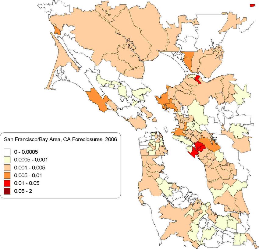
I
                       Are Foreclosures Contagious?
Ryan M. Goodsteina , Paul Hanounab,e , Carlos D. Ramirezc,e , Christof W. Staheld,e,∗
          a
              Division of Insurance and Research, Federal Deposit Insurance Corporation
                             b
                               Department of Finance, Villanova University
                        c
                          Department of Economics, George Mason University
                          d
                            Department of Finance, George Mason University
               e
                 Center for Financial Research, Federal Deposit Insurance Corporation

Abstract
Using a large sample of U.S. mortgages observed over the 2005-2009 period, we find that foreclo-
sures are contagious. After controlling for major factors known to influence a borrower’s decision
to default, including borrower and loan characteristics, local demographic and economic conditions,
and changes in property values, the likelihood of a mortgage default increases by as much as 24%
with a one standard deviation increase in the foreclosure rate of the borrower’s surrounding zip code.
We find that foreclosure contagion is most prevalent among strategic defaulters: borrowers who are
underwater on their mortgage but are not likely to be financially distressed. Taken together, the
evidence supports the notion that foreclosures are contagious.

Keywords: Foreclosure, Contagion, Mortgages, Learning, Stigma

   I
      We would like to thank, without implicating, Sanjiv Das, Enrica Detragiache, James Einloth,
Paul Kupiec, Myron Kwast, Haluk Ünal and Erlend Nier, as well as seminar participants at the MCM
seminar at the International Monetary Fund and the FDIC for helpful comments and suggestions.
We gratefully acknowledge financial and logistical support from the Center for Financial Research
at the FDIC. The views expressed in this paper do not necessarily reflect those of the Federal Deposit
Insurance Corporation.
    ∗
      Corresponding Author
      Email addresses: rgoodstein@fdic.gov (Ryan M. Goodstein),
paul.hanouna@villanova.edu (Paul Hanouna), cramire2@gmu.edu (Carlos D. Ramirez),
cstahel@gmu.edu (Christof W. Stahel)

                                                                                    January 19, 2011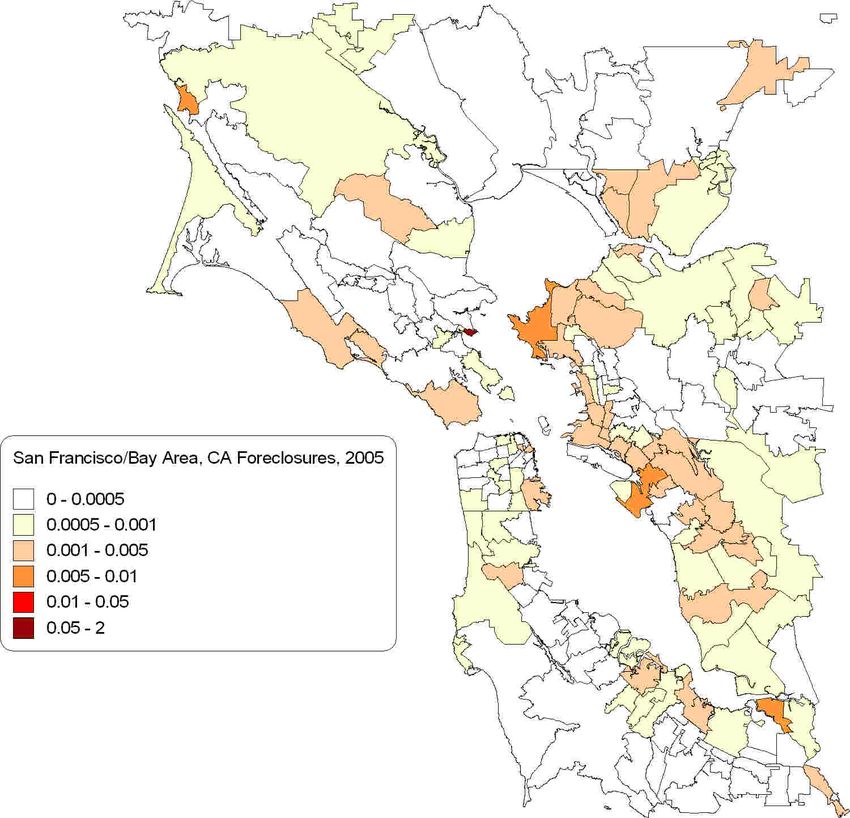
1. Introduction
It is well understood that the origins of the ongoing U.S. financial crisis lie
in the inordinate number of mortgage delinquencies triggered, at least in part, by
the collapse of the real estate market.1 The resulting large number of underwater
borrowers coupled with the economic recession has led to a sharp increase in fore-
closure activity, reaching levels not seen for at least the last 60 years (see figure 1).
This spike in foreclosures has led to numerous reports in the popular press about
the presence of “foreclosure contagion”.2 Although claims of “contagion” might
be dismissed as sensationalism, they could also be attributed to the observation that
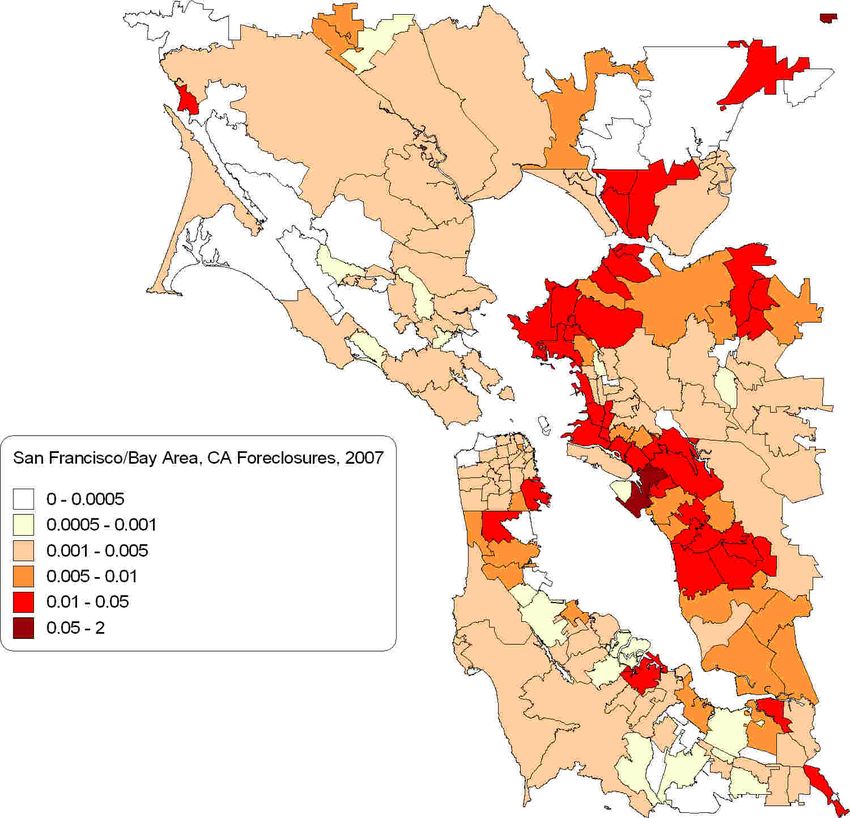
foreclosures tend to cluster around and spread from various loci. To illustrate, fig-
ure 2, tracking the evolution of foreclosure rates in the San Francisco-Bay Area
from 2005 through 2008, clearly displays these patterns. However, observing that
defaults tend to cluster is not sufficient to determine the existence of contagion since
these clusters could be the result of common circumstances among borrowers such
as local economic shocks.
Mortgage defaults are contagious if they directly increase the default probability
of another mortgage on a nearby property, all else held constant. The academic lit-
erature provides little systematic evidence as to whether foreclosures are contagious
and the mechanisms that would render them contagious. By and large, the common
view has been that foreclosures are primarily determined by a borrower’s inability
1
See, for example, Brunnermeier (2009) and Gorton (2009) for excellent discussions on the
causes of the recent financial crisis.
2
An Internet search on the terms “subprime contagion,” “mortgage contagion” or “foreclosure
contagion” returns results in the millions as the popular press relayed the wave of mortgage defaults
in such terms. For example, an article headline in Bloomberg News reads “Subprime Contagion May
Claim 10-Year Treasuries as Next Victim” (Bloomberg News: November 5, 2007) while another in
the Boston Globe states “A foreclosure virus spreads.” (Boston Globe: February 15, 20080).
2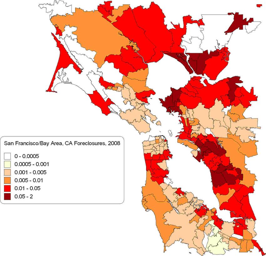
to pay and therefore any correlation among defaults was interpreted as originat-
ing from common factors affecting economic conditions. Recent evidence that at
least some of the large pool of underwater borrowers have strategically defaulted
on their mortgages allows for other interpretations.3 Based on survey data, Guiso,
Sapienza, and Zingales (2009) find evidence that mortgage defaults are contagious:
other things equal, homeowners who know someone who defaulted are 82% more
likely to declare their willingness to strategically default. Our work complements
their findings in an important respect. While they establish the possibility that mort-
gage default contagion exists based on survey data, we provide evidence of such
contagion based on actual mortgage default data.
       We identify and measure the presence of foreclosure contagion by analyzing
a large sample of mortgages originated over the period 2000-2008 and observed
from 2005 to 2009. Specifically, we estimate the probability of default on a given
loan as a function of the foreclosure rate in zip codes adjacent to the property,
while controlling for economic fundamentals like borrower and loan characteristics,
changes in property values, economic and demographic conditions at the zip code
level, as well as time and state fixed effects. We interpret a positive and significant
impact of the area foreclosure rate on the probability of default as contagion. This
interpretation is consistent with the one used in the finance literature, which defines
contagion as correlation over and above that expected from economic fundamentals
(e.g. Bekaert, Harvey, and Ng, 2005; Boyson, Stahel, and Stulz, 2010). We find
that an increase in the foreclosure rates in zip codes within 5 miles of a property

   3
     According to Fannie Mae’s National Housing Survey (2010), 20% of homeowners report know-
ing at least one person who stopped making monthly mortgage payments despite being able to afford
it. Oliver Wyman (2009) reports that strategic defaulters make up 18% of all borrowers who went
60 days on their mortgage in the fourth quarter of 2008.

                                               3
significantly raises the probability of default of a given loan at the 1% significance
level after controlling for the large set of covariates. Our estimates suggest that a
one standard deviation increase in the area foreclosure rate increases the probability
of a mortgage default by up to 24%. The results are robust to various specifications
and estimation methods. Specifically, they are robust to using the first incidence of
90+ days delinquency instead of the foreclosure event as the measure of default, an
observation worth making because of the concern that the foreclosure event may
not be entirely determined by the borrower.
Our results indicate that the contagion effect is much stronger for borrowers who
are underwater but less likely to be financially distressed. To identify a “potential
strategic defaulter”, we first require the mortgage to be significantly underwater,
and second, we condition on one of the following three characteristics: Fair Is-
sac (FICO) credit scores, relative property values, and relative per capita incomes.
We find that borrowers with current Loan-to-Value (LTV) ratios on their homes of
above 120% and FICO scores above 720 are six times more likely to be influenced
by surrounding area foreclosures relative to the magnitude found for lower LTV
ratios and lower FICO scores. We find similar results when the sample is stratified
by property values or by per capita incomes.
The finding that contagion is prevalent among potential strategic defaulters and
not among those who are more likely to be financially distressed is plausible and
intuitive. Financially distressed borrowers default because they lose their ability to
make continued payments. Since they have little or no choice in the matter, their
default is less likely to be a function of other defaults, and instead a function of com-
mon adverse economic conditions. In contrast, strategic defaulters do so because
their willingness to make continued payments declines. Therefore, contagion in this
4group occurs because their willingness to keep making payments is undermined by
other defaults.
Because of obvious policymaking implications, measuring and quantifying fore-
closure externalities has mushroomed into an important area of research in recent
years. For example, Immergluck and Smith (2006a), Harding, Rosenblatt, and Yao
(2009), and Campbell, Giglio, and Pathak (2009) find that, holding all else constant,
foreclosed homes significantly decrease the property values of nearby homes. No-
tably, Harding, Rosenblatt, and Yao (2009) highlight the negative externalities that
foreclosures have by disproportionally depressing the property values of nearby
homes. These papers have made significant inroads in the literature, but they do
not specifically investigate to what extent and how foreclosures are responsible for
directly causing other homeowners to default beyond the possible price contagion
channel emphasized by Harding, Rosenblatt, and Yao (2009). The channels through
which foreclosures directly affect the default decision, even after controlling for
price effects, are what we label “non-price” contagion channels.
Our results are consistent with at least three possible, non-mutually exclusive
mechanisms of non-price default contagion. First, abstracting from borrower moral-
ity, in the case of deeply underwater properties homeowners can reap substantial
long term benefits from walking away from their homes (e.g. Foster and Van Or-
der, 1984; Deng, Quigley, and Van Order, 2000). Nonetheless, the decision to walk
away from a home is likely to be a difficult choice for most households, and more-
over, homeowners might be unaware of their option to strategically default or of
the cost thereof. Neighbors who default on their mortgage can help potential strate-
gic defaulter navigate the process with credible and visible information. Learning
through the experience of others, especially when it relates to foreclosures, may be
5more powerful and more cost effective than learning through the media, accoun-
tants, or lawyers. At the very least, observing a nearby neighbor who defaulted
provides concrete, and locally sensitive, information about the consequences of de-
fault. We label this mechanism the “learning channel.” 4
Second, insofar as moral considerations affect the willingness to default, moral-
ity may be relative; the more people default, the less morally objectionable it may
become (see, for example, Guiso, Sapienza, and Zingales, 2009). Thus, to the ex-
tent that borrower morality enters into the decision to default, when defaults become
locally systemic the role of morality declines, thereby lowering the “social cost” of
further defaults. A similar argument can be made about social stigma, that is the
fear of being an outcast, associated with default (see, for example, Blume, 2010).
Stigma declines with the proportion of people defaulting, and as a result, the cost
of further defaults becomes increasingly smaller.
Third, a potentially important consideration in the homeowners’ willingness
to make continued payments on an “underwater” mortgage is the loss of social
networks and the degradation of public infrastructure and security caused by high
neighborhood foreclosure rates (see, for example, Immergluck and Smith, 2006b;
Goodstein and Lee, 2010). We call this last mechanism the “social network chan-
nel.”
A typical concern that arises in empirical studies similar to ours is the possibility
that the results could be driven by an omitted variable. There are at least three
reasons that render such a bias unlikely in our analysis. First, to compromise our
4
This mechanism implicitly assumes that potential strategic defaulters systematically overesti-
mate the cost of default, and that, by observing others default, they update those estimates down-
wards. Although we do not formally model this process, such “overestimation” can be the result of
risk aversion.
6results, the omitted variable would have to be uncorrelated with the area property
values or local economic shocks (and an extensive number of lags), since these
variables are included as controls in all of our specifications. Second, we find that
the borrower’s default decision is correlated with foreclosures within 0 to 5 miles of
the property, but not with foreclosures in a slightly more distant area, 5 to 10 miles
from the property. To the extent that economic conditions in a borrower’s local area
are similar to those faced by borrowers 5 to 10 miles away, the omitted variable
would have rendered the 5 to 10 mile foreclosure rate statistically significant as well.
Third, in all three different stratification criteria we use for identifying strategic
defaulters (FICO, property value, and per capita income), we find that the area
foreclosure rate is not an economically significant driver of mortgage defaults for
financially distressed borrowers. This result attests to the absence of an omitted
variable as the controls included in our specifications suffice to explain the default
decision of distressed borrowers.
The rest of this paper is organized as follows. The following section 2 presents
the data. Section 3 discusses the empirical methodology and section 4 reports the
results. Section 5 concludes.
2. Data
Our sample of mortgage loans comes from proprietary data assembled by Lender
Processing Services Inc. (LPS), formerly known as McDash. LPS consists of loan-
level information provided by participating mortgage servicing firms, including (by
year-end 2009) nine of the ten largest firms and 16 in total, reporting on over 30
million active loans. The LPS data include a rich set of loan characteristics at orig-
ination, including loan amount, property value, loan terms, and interest rate and
7amortization terms. LPS also contains for each loan a monthly payment record that
can be used to measure payment performance of the loan and foreclosure status.
LPS does have some important limitations. Although LPS’ coverage of the U.S.
mortgage market is strong overall, it is not a random sample of the market and
some segments of the market, such as subprime mortgages are under-represented.5
Due to the massive size of LPS data, we draw a random sample of loans for
use in our analysis (e.g. Foote, Gerardi, Goette, and Willen, 2009). We restrict
our sample of loans to owner-occupied, first-lien home purchase mortgages on 1-4
family homes. Moreover, we retain only loans where the property is located in a zip
code for which we have monthly zip code level house price information from Case-
Shiller. The loans in our sample were originated between years 2000 and 2008,
and we examine mortgage default behavior over the period January 2005 to March
2009.6
Separately, we compute “local area” foreclosure rates by zip code and month
from January 2005 to March 2009, using the full LPS dataset.7 Specifically, we first
compute foreclosure rates at the zip code level, where the foreclosure rate in the zip
code for a given month is defined as the count of mortgage loans in foreclosure
(payment status equal to “foreclosure pre-sale”, “foreclosure post-sale”, or “REO”)
5
Immergluck (2008) reports that, as of year-end 2008, LPS covered roughly 58 percent of the
total prime/near prime market and 32 percent of the subprime market.
6
We draw the random sample as follows. First, we drop all loans from LPS that are not owner-
occupied, first lien, 1-4 family, home purchase loans. We then remove all loans originated prior to
year 2000 or that were not active in at least one month in January 2005 or later. Next, we remove
loans for which we have no payment records within the first 12 months from origination. Finally, we
drop loans on properties not located within the set of 4,110 zip codes covered by the Case-Shiller
zip-code level House Price Index. From these remaining loans we draw a random five-percent
sample.
7
We purge the data of all loans that are not first-lien, 1-4 family, purchase or refinance, and
owner-occupied before computing these foreclosure rates.
8divided by the count of all active loans. Then, for each zip code, we calculate
a (0, 5] mile area foreclosure rate, FCR00.05 , as the weighted average of zip code
foreclosure rates for all zip codes greater than zero and less than five miles away.8
Similarly, we compute a (5, 10] mile area foreclosure rate, FCR05.10 .
To control for local macro-economic conditions, we include monthly county-
level unemployment rates from the Bureau of Labor Statistics’ Local Area Unem-
ployment Statistics. Furthermore, we use the Case-Shiller zip code level house price
index along with the original property value and the current loan balance to impute
the current loan-to value ratio (LT V) for every loan-month observation in our sam-
ple. Since LPS does not include information on the presence of junior liens, we are
unable to compute the combined LT V ratio for the loans in our sample. Thus, we
are understating the true LT V for some loans in our sample.9 We control for this by
including a dummy variable reflecting an LT V equal to 80% at origination, which
serves as a proxy for the presence of a second lien (see Foote, Gerardi, and Willen,
2008). We also include the two-year house price change directly in the model to
control for the state of the housing market within the zip code and the price conta-
gion channel emphasized by Harding, Rosenblatt, and Yao (2009) and Campbell,
Giglio, and Pathak (2009).10 Finally, we control for annual changes in county-level
demographic characteristics using Census Population Estimates.
To stratify the sample, we construct a “high property value zip code” indica-
8
Distances are based on the centroids of zip code areas. The zip code in which the property is
located is excluded when computing FCR00.05 .
9
Based on a sample of mortgages from LPS of first-lien, fixed rate originations in 2005-06
matched with credit bureau records, Elul, Souleles, Chomsisengphet, Glennon, and Hunt. (2010)
find that for the 26% of borrowers with a second mortgage, combined LT V is approximately 15
percentage points higher than LT V.
10
See also Nadauld and Sherlund (2009).
9tor, based on the median property value of a zip code relative to the median prop-
erty value of its corresponding metropolitan statistical area (MSA). The indicator
is equal to one if the zip code median property value is greater than 120 percent of
the MSA median property value. Similarly, we construct a “high per-capita income
zip code” indicator equal to one if the per-capita income of the zip code is greater
than 120 percent of MSA per-capita income. All property value and per-capita in-
come measures are from the 2000 Decennial Census. We drop from the sample all
loan-month observations with less than 100 active loans used to compute local area
foreclosure rates, and also drop loan-month observations with missing data for one-
to six-month lags of unemployment rates and house price changes. The final sample
consists of 168,542 unique loans for roughly 3.85 million loan-month observations.
Descriptive statistics are presented in Table 1. The raw hazard rate into fore-
closure across all loan-month observations in our sample is 0.3%, and 6.8% of
the loans in our sample enter foreclosure over our period of observation. Figure
3 presents baseline hazard rates, where loan-month observations are stratified into
four groups based on LT V (“High” if LT V is greater than 100, and “Low” other-
wise) and the area foreclosure rate (“High” if FCR is greater than or equal to 2.1,
the 75th percentile value of FCR, and “Low” otherwise). As expected, the figure
shows that the probability of entering foreclosure in a given month conditional on
not having entered foreclosure up to the prior month is substantially larger for the
two High LT V groups compared to the Low LT V groups. However, the baseline
hazard rate of High LT V loans is larger for those in High FCR areas compared to
Low FCR areas, suggesting that FCR may affect foreclosure decisions. Of course,
an alternative explanation is that this difference in hazard rates is driven by other
factors correlated with the FCR. We control for such factors in our econometric
10specification described in the next section.
3. Methodology
The standard “option model” of mortgage default includes interest rates and
house values as key explanatory variables. (see, for example, Foster and Van Order,
1984; Deng, Quigley, and Van Order, 2000). The simplest version of the model
implicitly assumes that the housing market is efficient in the sense that home prices
reflect all pertinent information about the market. Thus, home prices represent the
discounted present value of rational expectations of future rental income. Taken at
face value, the model implies that, in the absence of transaction costs, a borrower
should default when the market value of the promised mortgage payments exceeds
the market value of the house.
In reality information problems as well as transaction costs (which may well
be individual-specific), render the simple model incomplete. Thus, having negative
equity in the home may be a necessary but certainly not sufficient condition for
default. On one hand, in the absence of cash flow problems, an underwater borrower
might continue making payments perhaps because she is not aware of her options
to default, or she believes the act of defaulting is objectionable or simply too costly.
Consequently, several papers investigate the potential impact transaction costs have
on default (e.g. Foster and Van Order, 1984; Vandell, 1995). On the other hand,
a series of papers study the role cash flow problems, for example due to job loss
or divorce, may have in triggering default (Vandell, 1995; Gerardi, Shapiro, and
Willen, 2007; Foote, Gerardi, and Willen, 2008; Elul, Souleles, Chomsisengphet,
Glennon, and Hunt., 2010) because a borrower with negative equity that suffers such
a “trigger event” may be unable to continue making mortgage payments. Hence,
11more realistic models of mortgage default expand on the standard option model
and encompass a large set of explanatory variables, including those that measure
transaction costs and identify “trigger events.”
The more accepted definition of contagion in the finance literature is the notion
of excess correlation, or co-movement beyond what economic fundamentals can
explain (Bekaert, Harvey, and Ng, 2005), (Boyson, Stahel, and Stulz, 2010). In the
context of this paper, this definition implies that other foreclosures in the neighbor-
hood have an effect on the probability of a strategic default beyond what common
factors would predict. Therefore, to investigate whether foreclosure contagion ex-
ists, we augment an expanded model of mortgage default that contains a large array
of explanatory variables with the local area foreclosure rate. This allows us to iso-
late the effect of the neighborhood foreclosure rate on the probability to foreclose.
If the area foreclosure rate remains statistically significant after the inclusion of
these fundamental factors, we would have evidence in favor of contagion.
Specifically, we model the probability of default as follows:
h i
Pr(Di (t) = 1) = f FCRi (t − 1), Mi (0), L1,...,6 {LT Vi (t), UEMPi (t), ∆HPIi (t)} , Q(t)
where i indexes a loan and L1,...,6 {} is a polynomial in the lag operator generating
six lags of the variables in curly brackets. The dependent variable Di (t) takes on
a value of one in the first month in which the loan enters foreclosure, and is zero
otherwise.11
11
Loan-month observations following the first incidence of the loan entering foreclosure are
dropped. In an alternative specification we define default as the first incidence of 90+ days delin-
quency. The baseline estimates from this model – not shown – are qualitatively similar.
12The key independent variable FCRi (t − 1) is the one month lagged foreclo-
sure rate in the local area. After including all our control variables, we interpret
a positive coefficient on FCR as evidence in support of foreclosure contagion (see
Boyson, Stahel, and Stulz, 2010, for a similar approach). The controls in our model
include Mi , a vector of time-invariant measures characterizing the loan at origina-
tion. It includes indicators for interest rate type (fixed or not-fixed), loan purpose
(refinance or purchase), loan documentation, credit score (FICO), debt-to-income
ratio (DT I), and whether or not the loan-to-value (LT V) ratio at origination was ex-
actly equal to 80.12 In addition, all regressions include state fixed-effects. We also
include six lags of the time-varying controls in the model: (a) an estimate of current
loan-to-value ratio (LT V)13 ; (b) the county-level unemployment rate (UEMP) to
control for the likelihood that the borrower suffered an unexpected income shock;
and (c) the change in the house price over the prior two years (∆HPI), which may
reflect local macro-economic conditions as well as possibly proxy for borrower ex-
pectations of future house prices (see Nadauld and Sherlund, 2009). Finally, we
include state fixed-effects to control for persistent differences in observable and un-
observable factors across states, and quarterly fixed-effects to control for changes in
the national macro-economic conditions. We estimate the model using a dynamic
logit framework, allowing the associated hazard function to vary non-parametrically
by including a cubic spline in age. We cluster standard errors by zip code. For ro-
12
Nearly 25 percent of loans in our data had an LT V of 80 percent at origination. Foote, Gerardi,
and Willen (2008) note that these loans are likely to have been accompanied by a second lien. Thus
the combined LT V on these loans is likely higher than what we are able to compute from LPS data.
13
We enter LT V into our empirical specification as a series of indicator variables (less than 90;
between 90 and 100; between 100 and 110; and greater than 110). This categorization flexibly
controls for non-linearity in the impact of LT V on the decision to default.
13bustness, we also estimate the model using the Cox (1972) proportional hazard
framework.14
4. Results
We first estimate the baseline model and report in table 2 the estimated coeffi-
cients on the one-month lagged nearby FCR00.05 and distant FRC05.10 area foreclo-
sure rates along with the coefficients on the (one month lagged) control variables.
Both the dynamic logit model and the Cox proportional hazard rate model provide
similar results, suggesting that the findings are not sensitive to any particular estima-
tion technique.15 The coefficients suggest that after controlling for all other known
factors nearby foreclosures positively affect the decision to foreclose. The distant
area foreclosure coefficient is never statistically different from zero. Thus, we find
no evidence of contagion beyond the 0 to 5 mile radius. Inside of this narrower
radius, however, all estimated coefficients are positive and statistically significant.
The corresponding elasticity, ∂ ln[P(Di (t) = 1)]/ ∂ ln[FCRi (t − 1)], is 0.029 with
a z-value of 5.40. Given that the area foreclosure rate has a standard deviation of
3.02%, the elasticity estimate suggests that a one standard deviation shock in FCR
increases the foreclosure probability by more than 4.8% (= 0.029 × 3.02/1.82 × 100).
The proportional hazard model elasticity estimates are very similar. Since the base-
line results are quite similar across the estimation methods, we subsequently focus
14
Econometrically, the dynamic logit framework is closely related to the Cox proportional hazard
model. See, for example, Sueyoshi (1995) or Shumway (2001) for a discussion.
15
In order to compare coefficients, one needs to subtract 1.00 from the estimates of the propor-
tional hazard model. In unreported results, we also estimate the competing risk model advocated by
Deng, Quigley, and Van Order (2000), which accounts for the possibility that a loan may terminate
due to prepayment prior to a default being observed. These results are qualitatively similar.
14on the dynamic logit model only.
The results in Table 2 indicate that the probability of default is influenced by the
nearby area foreclosure rate. Although suggestive, these results do not necessarily
point to the existence of contagion. Why not? For contagion to be an explanation,
the borrowers must have the choice to default. Hence, to make the case for conta-
gion, we need to show that the nearby area foreclosure rate affects strategic defaults
– that is, foreclosures where mortgage holders choose to default on their obliga-
tions because their properties are underwater and the perceived cost of staying in
the house is larger than the perceived benefit.
Of course, identifying precisely the subset of borrowers who have the choice
to default for strategic reasons is virtually impossible. Even with a detailed dataset
on individual characteristics, it would be difficult to identify a borrower’s true in-
tentions and ability to pay. Still, it is possible to develop an identification strategy
based on borrower and loan characteristics as well as neighborhood conditions. We
start by concentrating on the subset of borrowers with high LT V ratios because a
strategic default makes sense only for underwater borrowers. However, while loans
with LT V above 100% are technically underwater, existing evidence suggests that
in practice LT V must be higher before a borrower exercises his option to strategi-
cally default. Guiso, Sapienza, and Zingales (2009) find, using survey data, that
strategic foreclosures are unlikely to take place for properties that are less than 10%
under water. Bhutta, Dokko, and Shan (2010) find that for subprime borrowers
in Arizona, California, Florida, and Nevada, the median strategic defaulter has an
LT V of 162% and 90% of strategic defaulters have an LT V of 120% or more. Based
on this evidence, we choose 120% as the threshold for “high” LT V over which a
15borrower might choose to strategically default.16 We thus create a dichotomous
variable equal to 1 if LT V is 120% or more, 0 otherwise.
Being significantly underwater alone does not necessarily ensure that we are
capturing borrowers who have the choice to default. We need to further identify
borrowers that less likely experience a cash flow shock or, if they do, are less likely
to be liquidity constrained after suffering such a shock. We use three alternative
measures to proxy for (lack of) liquidity constraints: the borrower’s FICO score
at origination of the loan, per capita income of the property zip code relative to its
MSA, and the median property value of the zip code relative to its MSA.
4.1. LT V and FICO Scores
We begin by allowing the effect of the local foreclosure rate on the borrower’s
probability to default to vary by LT V and FICO categories. Specifically, we add
interaction terms of FCR with indicators for “high” LTV and “high” FICO to the
empirical specification. Our focus is on the “high” LT V and “high” FICO group.
After controlling for all known factors determining foreclosure, one can reasonably
make the claim that default is more of a choice for this group of borrowers. There-
fore, we expect our contagion measure, FCR, to be significantly more important
for this group. In contrast, we expect foreclosure contagion to be much weaker for
other groups, in particular, those whose LT V ratios are not deemed to be “high”
and also have relatively low FICO scores.
Table 3 presents the estimated nearby area foreclosure rate effects on the proba-
bility of default, broken down by LT V (high or not) and FICO scores (high or not).
16
Our results (not shown) are similar when alternatively defining “high LTV” as greater than
130%.
16The effects are reported as elasticities to ensure comparability across the four buck-
ets and are based on the dynamic logit model discussed above. For the high FICO
and high LT V group, which we hypothesize is the group with the highest chance
of generating contagion, the estimated elasticity is 0.114, which is statistically dif-
ferent from 0 at the 1% level. This figure is 6 times larger than the one estimated
for low FICO and low LT V (which is 0.019). In addition, the difference between
these two estimated elasticities is statistically significant at the 5% level. Thus, the
evidence indicates the existance of contagion among those who are underwater and
have the choice to default.
4.2. LT V and Area Per Capita Income
The second breakdown considered is the LT V and the area per capita income.17
Intuitively, it is natural to think that in relatively poorer neighborhoods – those
where income per capita tends to be low – the incidence of financially distressed
borrowers is higher than in high per capita income areas, or that a homeowner’s abil-
ity to continue making payment is more susceptible to income shocks. It follows
that strategic default is more likely in relatively wealthier neighborhoods. Follow-
ing this logic, one would expect to observe a higher level of foreclosure contagion
among borrowers who are underwater and reside in a relatively wealthier neighbor-
hood.
Paralleling the breakdown of the prior table, Table 4 presents the nearby fore-
closure area elasticities split by LT V levels (high or not) and area per capita income
(high or not). The reported effects are qualitatively similar to those observed in Ta-
17
See section 2 for the definition of high property value zip code indicator on which the stratifi-
cation is based.
17ble 3. For the high LT V and high per capita income subset the estimated elasticity
(0.245) is nearly 19 times larger than the one estimated for the low per capita in-
come, low LT V bucket (0.013). The χ2 test indicates that these two elasticities are
statistically different from each other at the less than 1% significance level. The off-
diagonal elasticities tend to also be relatively small, although they are statistically
significant. Thus, overall, this second way of stratifying the sample delivers results
that are consistent with the hypothesis that foreclosure contagion is more relevant
for strategic defaulters.18
4.3. LT V and Property Value
Our third stratification is by LT V and whether or not the property is located
in a high property value area zip code.19 Just as in the LT V and area per capita
income breakdown, this way of splitting the sample attempts to isolate the group
of borrowers who are more likely to view the decision to default as a strategic
decision. We hypothesize that a borrower who is underwater and whose property is
located in a relatively more expensive neighborhood is more likely to be a strategic
defaulter, relative to the low LT V and low property value group. This reasoning
follows the fact that in poorer neighborhoods mortgage default is less likely to be
done by choice but more likely to be done by necessity.
The results presented in Table 5 are quite consistent with this intuitive expla-
nation and are similar to the ones from the previous stratifications. For the high
18
Indeed, a recent article in The New York Times offer anecdotal evidence for this re-
sult: “... many of the well-to-do are purposely dumping their financially draining properties,
just as they would any sour investment.” http://www.nytimes.com/2010/07/09/business/
economy/09rich.html
19
The stratification follows the construction of the area per capita income subset but uses the high
property value indicator variable introduced in section 2.
18LT V and high property value group the estimated elasticity is 0.116, while the one
for low LT V, low property value group is a statistically insignificant 0.009. Not
surprisingly, the difference between these two estimated elasticities is statistically
significant at the 5% level. Thus, broadly speaking, all three stratifications point in
the same direction: contagion is more prevalent among strategic defaulters.
4.4. Contagion non-linearities
In the introduction we highlighted three non-mutually exclusive channels by
which contagion might spread. While our primary interest is to show the existence
of contagion and not to test for specific channels, finding results consistent with the
conjectured mechanisms supports the notion of foreclosure contagion. Neverthe-
less, each mechanism further suggests that the contagion effect should accelerate
in the area foreclosure rate. For example, contagion through learning takes place if
a foreclosure event in the neighborhood allows underwater homeowners to update
their knowledge about the consequences of defaulting on a mortgage. This mech-
anism implies that foreclosures may breed further foreclosures in the same area,
because people learn more about foreclosures (and its consequences) from each
other. Hence, we would expect to observe “contagion acceleration” – as the area
foreclosure rate rises, contagion accelerates.20
The stigma generated by foreclosure and the moral issues associated with de-
fault are two other mechanisms through which foreclosure contagion could spread,
and they are also affected by the magnitude of the area foreclosure rate. In particu-
lar, both stigma and moral concerns ought to decline with a higher area foreclosure
20
This argument implicitly assumes that borrowers systematically overestimate the cost of de-
faulting, which is reasonable under risk aversion.
19incidence. Why? As the area foreclosure rate rises, the social network that enforces
stigma and moral issues about default weakens. As a result, just as with the learning
channel, we would expect to observe “contagion acceleration” in the data.
To examine whether or not “contagion acceleration” is present in the data we
further include in the regression model the square term of the area foreclosure rate
and estimate the elasticities at different levels of the area foreclosure rate. If “con-
tagion acceleration” is present, as the area foreclosure rate increases the estimated
elasticity should rise as well. Table 6 presents two sets of results: one for all bor-
rowers and one for those who are most likely the strategic defaulters (high LT V and
high FICO scores). Both columns present similar results – the elasticity rises as the
area foreclosure rate increases. When the area foreclosure rate is small (0.50), the
estimated area foreclosure elasticity is only 0.021 for all borrowers, and 0.018 for
the strategic defaulters. But as the area foreclosure rate rises, the estimated elas-
ticity monotonically increases to 0.171 for all borrowers and 0.147 for the strategic
defaulters. These numbers imply that a one standard deviation increase in the area
foreclosure rate increases the probabilities by 28.4% and 24.4%. A χ2 test reveals
that the highest estimated elasticity and the smallest one are indeed statistically dif-
ferent at the 1% level for all borrowers and the 5% level for the strategic defaulters.
5. Conclusion
We use a large sample of U.S. mortgages observed between 2005 and 2009 to
investigate foreclosure contagion. We define contagion as the impact that nearby
foreclosures have on the conditional probability of a mortgage default after control-
ling for all other known determinants, including house price appreciation, which
Harding, Rosenblatt, and Yao (2009) and Campbell, Giglio, and Pathak (2009)
20highlight as being important drivers of default. The results show that foreclosures
do indeed breed further foreclosures. Specifically, we find that holding everything
else constant, a 1% increase in the foreclosure rate of surrounding zip codes (within
a radius of 5 miles), increases the likelihood of an individual mortgage default by
0.029%. The results are not only statistically significant, but economically impor-
tant: the estimated elasticity implies that a one standard deviation increase in the
area foreclosure rate translates into a 4.81% increase in the probability of default
for our baseline model and as much as 24% for other specifications. It is unlikely
these results are driven by an omitted variable problem given the battery of con-
trols in the model and the inclusion of the foreclosure rate within a 5 to 10 mile
radius, an area most likely experiencing the same overall economic conditions as
our variable of interest. In that respect, the insignificance of the 5 to 10 mile radius
area foreclosure rate in the regressions is comforting given that an omitted variable
problem should render it significant.
We discuss three non-mutually exclusive mechanisms by which foreclosure
contagion can take place: (1) a learning channel, (2) a social capital channel, and
(3) a social network channel. The commonality among all three channels is that
foreclosures either provide underwater homeowners informational updates as to the
consequences of strategically defaulting or influence their willingness to stay cur-
rent.
Evidence of foreclosure contagion has important financial and economic rami-
fications. First, with an outstanding amount approaching $14.3 trillion,21 the U.S.
residential mortgage debt market is economically as significant as the U.S. corpo-
21 th
4 Quarter 2009, Mortgage debt outstanding, Board of Governors of the Federal Reserve Sys-
tem.
21rate debt market22 and, as discussed above, has been at the heart of the current U.S.
financial crisis. Yet, while there has been much work on identifying and explain-
ing contagion effects in corporate credit markets, the same question has remained
largely unaddressed in the residential debt markets.23 Second, contagion has obvi-
ous implications for the pricing and design of mortgage contingent securities such
as Mortgage-Backed Securities (MBS) and Collateralized Mortgage Obligations
(CMO). If properly understood, contagion effects among the loans composing the
MBS pool might be mitigated. Third, understanding the nature of the correlation
among mortgage defaults can be a significant input in determining the loan port-
folio risk of banks as is required by the Basel III accords and is therefore directly
relevant to banking regulatory agencies. In particular, foreclosure contagion can be
an important element in the current debate on the size of individual banking units.
Indeed, if foreclosures are contagious an argument can be made for banks to be suf-
ficiently large and geographically diversified as to be able to withstand that effect.
Finally, the proper understanding of homeowners’ decision to default is critical in
designing home-loan modification programs and solving real estate based financial
crises.
Finally, establishing the presence of foreclosure contagion is a novel result,
which has important implications for banks, bank regulators, policymakers, and
credit market participants. Moreover, it provides insight into how households learn,
process, and transmit information.
22
The Bureau of International Settlements reports U.S. Corporate Debt at approximately $15.6
trillion in the 4th Quarter of 2009.
23
Das, Duffie, Kapadia, and Saita (2007) and Jorion and Zhang (2007) for example find evidence
of contagion in the corporate bond market.
22References
Bekaert, Geert, Campbell R. Harvey, and Angela Ng, 2005, Market Integration and
Contagion, The Journal of Business 78, 39–69.
Bhutta, Neil, Jane Dokko, and Hui Shan, 2010, The Depth of Negative Equity and
Mortgage Default Decisions, Finance and Economics Discussion Series, Federal
Reserve Board, No. 2010-35.
Blume, Lawrence E., 2010, Stigma and Social Control, Cornell University Working
Paper.
Boyson, Nicole, Christof Stahel, and Rene Stulz, 2010, Hedge Fund Contagion and
Liquidity Shocks, Journal of Finance 65, 1789–1816.
Brunnermeier, Markus K., 2009, Deciphering the Liquidity and Credit Crunch
2007-2008, Journal of Economic Perspectives 23, 77–100.
Campbell, John Y., Stefano Giglio, and Parag Pathak, 2009, Forced Sales and House
Prices, NBER Working Paper No. 14866.
Cox, David R., 1972, Regression models and life-tables (with discussion), Journal
of the Royal Statistical Society, Series B 34, 187–220.
Das, Sanjiv, Darrell Duffie, Nikunj Kapadia, and Leandro Saita, 2007, Common
failings: How corporate defaults are correlated, Journal of Finance 62, 93–118.
Deng, Yongheng, John M. Quigley, and Robert. Van Order, 2000, Mortgage Ter-
minations, Heterogeneity, and the Exercise of Mortgage Options., Econometrica
68, 275–307.
Elul, Ronel, Nicholas S. Souleles, Souphala Chomsisengphet, Dennis Glennon, and
Robert Hunt., 2010, What Triggers Mortgage Default?, Working Paper 10-13,
Research Department, Federal Reserve Bank of Philadelphia.
Foote, Christopher L., Kristopher Gerardi, Lorenz Goette, and Paul S. Willen, 2009,
Reducing Foreclosures: No Easy Answers, Federal Reserve Bank of Atlanta
Working Paper 2009-15.
23Foote, Christopher L., Kristopher Gerardi, and Paul S. Willen, 2008, Negative eq-
uity and foreclosure: Theory and evidence, Journal of Urban Economics 64,
234–245.
Foster, Chester, and Robert. Van Order, 1984, An Option-Based Model of Mortgage
Default, Housing Finance Review 3, 351–372.
Gerardi, Kristopher, Adam Hale Shapiro, and Paul S. Willen, 2007, Subprime Out-
comes: Risky Mortgages, Homeownership Experiences and Foreclosures., Fed-
eral Reserve Bank of Boston Working Paper.
Goodstein, Ryan M., and Yan Y. Lee, 2010, Do Foreclosures Increase Crime?,
FDIC Center for Financial Research Working Paper No. 2010-05.
Gorton, Gary B., 2009, Information, Liquidity, and the (Ongoing) Panic of 2007,
American Economic Review 99, 567–572.
Guiso, Luigi, Paola Sapienza, and Luigi Zingales, 2009, Moral and Social Con-
straints to Strategic Default on Mortgages, NBER Working Paper No. 15145.
Harding, John P., Eric Rosenblatt, and Vincent W. Yao, 2009, The Contagion Effect
of Foreclosed Properties, Journal of Urban Economics 66, 164–178.
Immergluck, Dan, 2008, The Accumulation of Foreclosed Properties: Trajectories
of Metropolitan REO Inventories During the 2007-2008 Mortgage Crisis., Com-
munity Affairs Discussion Paper No. 02-08, Federal Reserve Bank of Atlanta.
Immergluck, Dan, and Geoff Smith, 2006a, The External Costs of Foreclosure: The
Impact of Single-Family Mortgage Foreclosures on Property Values, Housing
Policy Debate 17, 57–79.
Immergluck, Dan, and Geoff Smith, 2006b, The Impact of Single-family Mortgage
Foreclosures on Neighborhood Crime, Housing Studies 21, 851–866.
Jorion, Phillippe, and Gaiyan Zhang, 2007, Good and Bad Credit Contagion: Evi-
dence from Credit Default Swaps., Journal of Financial Economics 84, 860–883.
Nadauld, Taylor, and Shane M. Sherlund, 2009, The Role of the Securitization
Process in the Expansion of Subprime Credit, SSRN eLibrary.
Shumway, Tyler, 2001, Forecasting Bankruptcy More Accurately: A Simple Haz-
ard Model, The Journal of Business 74, 101–124.
24Sueyoshi, Glenn T., 1995, A Class of Binary Response Models for Grouped Dura-
tion Data, Journal of Applied Econometrics 10, 411–431.
Vandell, Kerry, 1995, How Ruthless is Mortgage Default? A Review and Synthesis
of the Evidence, Journal of Housing Research 6, 245–264.
253
Foreclosure Rate (%)
2
1
0
1950 1960 1970 1980 1990 2000 2008
Figure 1: Historical foreclosure rates (1950-2008). Source: Mortgage Bankers Association.
26Figure 2: Foreclosure Rates in the San Francisco Bay Area 2005-2008. Source: Authors’ calcula-
tion.
27·10−2
2
1.5
Hazard rate
1
0.5
0
10 20 30 40
Months from origination
High LTV, Low Area FCR High LTV, High Area FCR
Low LTV, High Area FCR Low LTV, Low Area FCR
Figure 3: Baseline hazard rates into foreclosure by LT V and area foreclosure rate.
A loan is categorized as “High LT V” in month t if LT V is greater than or equal to 120, and catego-
rized as “Low LTV” otherwise. A loan is categorized as “High FCR” if the foreclosure rate within 0
to 5 miles is greater than or equal to 2.6 (the value of FCR at the 75th percentile), and categorized as
“Low FCR” otherwise. Each line represents the predicted value from a regression of the raw hazard
rate on a cubic function of loan age. Regressions are estimated separately for each LT V-FCR group.
28Table 1: Descriptive Statistics
No. of subjects: 168,542
No. of records: 3,852,086
Failures: 11,395
Panel A: Time Invariant Variables (at origination)
Variable Mean Std. Deviation Min Max
Fixed Rate 65.193 47.635 0 100
Refinance 0 0 0 0
Full Documentation 28.915 45.337 0 100
Low or No Documentation 28.050 44.925 0 100
No info on Documentation 43.034 49.513 0 100
Credit Score: Low (less than 640) 7.822 26.852 0 100
Credit Score: Medium (between 640 and 720) 30.514 46.047 0 100
Credit Score: High (720 or more) 46.852 49.900 0 100
Credit Score: Missing 14.812 35.522 0 100
DTI: less than 28 34.953 47.682 0 100
DTI: between 28 and 36 15.577 36.264 0 100
DTI: between 36 and 42 13.855 34.548 0 100
DTI: 42 or more 14.779 35.489 0 100
DTI: Missing 20.835 40.613 0 100
Indicator: LTV equal to 80 at Origination 27.186 44.492 0 100
Share of Loans in High Property Zip Codes 34.561 47.557 0 100
Share of Loans in High Per Capita Income Zip Codes 33.066 47.045 0 100
Panel B: Time Variant Variables
Variable Mean Std. Deviation Min Max
Share of Loan-Month Obs in Foreclosure 0.302 5.492 0 100
Foreclosure Rate within 0-5 Miles, FCR00.05 , lag 1 mo 1.820 3.019 0 57.034
Foreclosure Rate within 5-10 Miles, FCR05.10 lag 1 mo 1.831 2.372 0 33.470
House Price Percentage Change over past 2 years 4.114 27.092 -75.470 107.118
Unemployment Rate 5.368 1.962 2.400 27.200
Indicator: LT V between 90 and 100 7.942 27.040 0 1
Indicator: LT V between 100 and 110 4.892 21.569 0 1
Indicator: LT V of 110 or more 6.725 25.045 0 1
County Population Share: Minority 23.015 11.140 3.223 71.957
County Population Share: Hispanic 20.045 14.783 0.880 77.313
County Population Share: Age less than 30 41.197 3.479 23.672 51.566
County Population Share: Age 60 or more 16.550 3.197 8.986 43.227
All numbers are expressed in terms of percentages.
29Table 2: Effect of Area Foreclosure Rate on the Probability of Foreclosure.
All specifications include full set of time variant (with 6 lags) and time invariant regressors, as well
as time and state fixed-effects. Logit regressions also include a cubic spline in age to account for
temporal dependence. Regressions estimated on a sample of 168,542 loans (3,852,086 loan-month
observations). Standard errors are clustered by zip code. Logit estimates are the marginal effect
of a 100 basis points increase in area foreclosure rate on the probability of entry into foreclosure.
Cox Proportional Hazard estimates are interpreted as the proportional effect of a 100 basis points
increase in the area foreclosure rate on the hazard rate of foreclosure.
Dynamic Logit Cox Proportional Hazard
(1) (2) (1) (2)
FCR00.05 (t − 1) 0.017∗∗∗ 0.016∗∗∗ 1.016∗∗∗ 1.016∗∗∗
(0.003) (0.003) (0.003) (0.003)
FCR05.10 (t − 1) −0.006 0.999
(0.005) (0.005)
Fixed Rate Loan −0.884∗∗∗ −0.884∗∗∗ 0.4212∗∗∗ 0.422∗∗∗
(0.022) (0.022) (0.009) (0.009)
Low or No Documentation 0.503∗∗∗ 0.503∗∗∗ 1.619∗∗∗ 1.619∗∗∗
(0.028) (0.028) (0.045) (0.045)
Credit Score < 640 1.795∗∗∗ 1.795∗∗∗ 5.824∗∗∗ 5.824∗∗∗
(0.036) (0.036) (0.207) (0.207)
Credit Score between 640 and 720 1.001∗∗∗ (1.001)∗∗∗ 2.677∗∗∗ 2.677∗∗∗
(0.027) (0.027) (0.073) (0.073)
Credit Score Missing 0.904∗∗∗ 0.903∗∗∗ 2.385∗∗∗ 2.385∗∗∗
(0.0367) (0.037) (0.087) (0.087)
Debt to Income ratio between 28 and 36% 0.396∗∗∗ 0.396∗∗∗ 1.490∗∗∗ 1.491∗∗∗
(0.045) (0.045) (0.067) (0.067)
Debt to Income ratio between 36 and 42% 0.560∗∗∗ 0.560∗∗∗ 1.738∗∗∗ 1.738∗∗∗
(0.044) (0.044) (0.076) (0.076)
Debt to Income ratio > 42% 0.629∗∗∗ 0.629∗∗∗ 1.885∗∗∗ 1.885∗∗∗
(0.042) (0.042) (0.078) (0.078)
LT V = 80 0.286∗∗∗ 0.286∗∗∗ 1.315∗∗∗ 1.315∗∗∗
(0.022) (0.022) (0.028) (0.028)
Housing Price Appreciation −0.063∗∗∗ −0.062∗∗∗ 0.942∗∗∗ 0.942∗∗∗
(0.019) (0.019) (0.018) (0.018)
Unemployment Rate −0.053∗∗ −0.052∗∗ 0.944∗∗ 0.944∗∗
(0.027) (0.027) (0.026) (0.026)
LT V 90 - 100 % 0.667∗∗∗ 0.668∗∗∗ 1.940∗∗∗ 1.940∗∗∗
(0.063) (0.063) (0.121) (0.121)
LT V 100 - 110 % 0.764∗∗∗ 0.765∗∗∗ 2.103∗∗∗ 2.103∗∗∗
(0.085) (0.085) (0.176) (0.176)
LT V > 110% 0.861∗∗∗ 0.861∗∗∗ 2.290∗∗∗ 2.290∗∗∗
(0.105) (0.105) (0.236) (0.236)
Share of Minority 0.003∗∗ 0.003∗∗ 1.004∗∗ 1.004∗∗
(0.002) (0.002) (0.002) (0.002)
Share of Hispanic 0.008∗∗∗ 0.008∗∗∗ 1.008∗∗∗ 1.008∗∗∗
(0.001) (0.001) (0.001) (0.001)
Share of Age less than 30 0.017∗∗ 0.017∗∗ 1.011 1.011
(0.008) (0.008) (0.009) (0.009)
Share of Age 60 or more 0.009 0.009 1.005 1.005
(0.009) (0.008) (0.009) (0.009)
Number of Observations 3,852,068 3,852,068 3,852,068 3,852,068
Pseudo R2 0.145 0.145 − −
30Table 3: Stratified Sample, by LT V and FICO.
All coefficients are elasticities estimated through a logit regression which include the full set of time
variant (with 6 lags) and time invariant regressors, as well as time and state fixed-effects. Logit
regressions also includes a cubic spline in age to account for temporal dependence. Regressions
estimated on a sample of 168,542 loans (3,852,086 loan-month observations). Standard errors clus-
tered by zip code. FICO-High (-Low) corresponds to loans originated to borrowers with a FICO
score of 720 or above (below 720). LT V-High (-Low) corresponds to loans with current LT V of
120 or above (below 120).
FICO - High FICO - Low
LT V - High 0.114∗∗∗ 0.0645∗∗
(0.041) (0.025)
LT V - Low 0.0735∗∗∗ 0.019∗∗∗
(0.008) (0.007)
Time invariant control variables yes yes
Time variant control variables yes yes
Time and state fixed effects yes yes
χ2 0.018∗∗
Table 4: Stratified Sample, by LT V and Per Capita Income.
All coefficients are elasticities estimated through a logit regression which include the full set of
time variant (with 6 lags) and time invariant regressors, as well as time and state fixed-effects. Logit
regressions also includes a cubic spline in age to account for temporal dependence. Regressions esti-
mated on a sample of 168,542 loans (3,852,086 loan-month observations). Standard errors clustered
by zip code. PCI-High (-Low) corresponds to loans originated in a zip code with per capita income
in the top (bottom three) quartile of all zip codes of a given MSA. LT V-High (-Low) corresponds to
loans with current LT V of 120 or above (below 120).
PCI - High PCI - Low
LT V - High 0.245∗∗∗ 0.051∗∗
(0.086) (0.022)
LT V - Low 0.068∗∗∗ 0.013∗
(0.009) (0.007)
Time invariant control variables yes yes
Time variant control variables yes yes
Time and state fixed effects yes yes
χ2 0.008∗∗∗
31You can also read