Universal role of commuting in the reduction of social assortativity in cities
←
→
Page content transcription
If your browser does not render page correctly, please read the page content below
Universal role of commuting in the reduction of social assortativity
                                                                              in cities
                                                          Eszter Bokányi1,2,∗ , Sándor Juhász1,2 , Márton Karsai3,4 , Balázs Lengyel1,2
arXiv:2105.01464v1 [physics.soc-ph] 4 May 2021

                                                             1
                                                             Corvinus University of Budapest; Laboratory for Networks, Technology and Innovation
                                                                                           Budapest, H-1093, Hungary
                                                 2
                                                   ELKH Centre for Economic and Regional Studies, Agglomeration and Social Networks Lendület Research Group
                                                                                           Budapest, H-1097, Hungary
                                                                    3
                                                                      Central European University; Department of Network and Data Science
                                                                                             Vienna, A-1100, Austria
                                                                                    4
                                                                                      Rényi Alfréd Institute of Mathematics,
                                                                                           Budapest, H-1053, Hungary
                                                                                ∗
                                                                                    Corresponding author: bokanyi.eszter@krtk.hu

                                                                                                    Abstract

                                                      Millions commute to work every day in cities and interact with colleagues, customers, providers,
                                                      friends, and strangers. Commuting facilitates the mixing of people from distant and diverse
                                                      neighborhoods, but whether this has an imprint on social inclusion or instead, connections
                                                      remain assortative is less explored. In this paper, we aim to better understand income sorting
                                                      in social networks inside cities and investigate how commuting distance conditions the online
                                                      social ties of Twitter users in the 50 largest metropolitan areas of the United States. Home and
                                                      work locations are identified from geolocated tweets that enable us to infer the socio-economic
                                                      status of individuals. Our results show that an above-median commuting distance in cities is
                                                      associated with more diverse individual networks in terms of connected peers and their income.
                                                      The degree that distant commutes link neighborhoods of different socio-economic backgrounds
                                                      greatly varies by city size and structure. However, we find that above-median commutes are
                                                      associated with a nearly uniform, moderate reduction of social tie assortativity across the top
                                                      50 US cities suggesting a universal role of commuting in integrating disparate social networks
                                                      in cities. Our results inform policy that facilitating access across distant neighborhoods can
                                                      advance the social inclusion of low-income groups.

                                                 1    Introduction
                                                 Cities are champions of diversity (Jacobs 2016; E. Glaeser 2011; Bettencourt 2013). Complex
                                                 interaction networks of individuals in urban areas enabled by population density, co-location, and
                                                 easy access together made cities the global engines of technological and economic progress (Duranton
                                                 and Puga 2020; Storper and Venables 2004; Calabrese et al. 2011a; Chong et al. 2020). However,
                                                 cities are also known for high levels of segregation (Sampson 2008; E. L. Glaeser, Resseger, and
                                                 Tobio 2009; Florida and Mellander 2015) where disparate neighborhoods are separated from each
                                                 other in the urban space (Ananat 2011; Chodrow 2017; Fry and Taylor 2012; Bokányi, Kondor, et al.

                                                                                                        1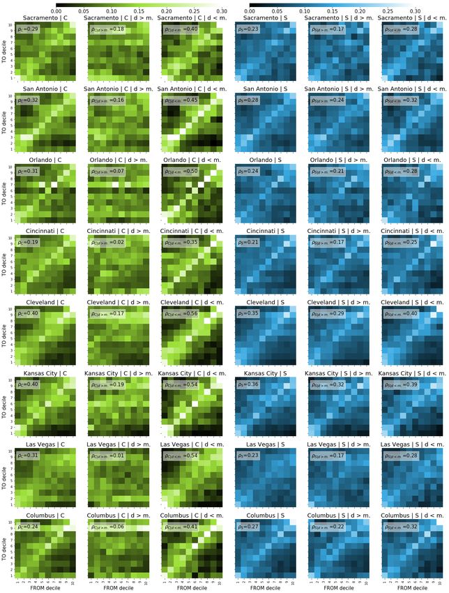
2016; Massey and Denton 1988). Furthermore, spatial segregation by income also fragments social
networks, which can hinder progress and can deepen inequalities (Eagle, Pentland, and Lazer 2009;
Bailey et al. 2020; Norbutas and Corten 2018; Abitbol and Karsai 2020; Tóth, Wachs, Clemente,
et al. 2019). Given the importance of this problem, a growing community has investigated the
patterns of mobility in cities to better understand mixing potentials across disparate and diverse
neighborhoods (Wang et al. 2018; Pappalardo et al. 2015; Dong et al. 2020; Heine et al. 2021), which
may increase economic prosperity (Eagle, Macy, and Claxton 2010). Yet, less is known whether
mobility mixing has any imprint on the social connections of people.
   Commuting covers a large share of urban mobility (Jiang et al. 2016) and by connecting home
with work locations, the places where people spend most of their time, it plays an important role
in the spatial formation of social connections (Dahlin, Kelly, and Moen 2008; Calabrese et al.
2011b; Small and Adler 2019). Since aggregated social networks form spatially bounded communi-
ties across neighborhoods (Bailey et al. 2020), the further one commutes, the higher the likelihood
that commuting-related social connections will introduce diversity in the egocentric network of the
commuter (Viry 2012; Blumenstock, Chi, and Tan 2019). Due to spatial segregation, economically
disparate neighborhoods tend to be far from each other (Roberto 2018), thus long commutes are
more likely to link places with different social status (Ham, Tammaru, and Janssen 2018; Nieuwen-
huis et al. 2020). Nevertheless, it is not trivial that long commutes should facilitate social inclusion,
because social interactions might remain assortative even at places far from home (Wang et al. 2018;
Morales et al. 2019; Dong et al. 2020). Meanwhile, the time to develop new social connections is
especially limited for low-income workers who travel to work during rush hours (Florez et al. 2016;
Dannemann, Sotomayor-Gómez, and Samaniego 2018).
   The spatial distribution of high versus low-income households determines the length of travel
that can bridge disparate neighborhoods. Since the scale of socio-economic isolation greatly varies
across cities (Chodrow 2017), one may expect that the mobility of people also enables a different
degree of social mixture. However, the assortativity of urban mobility is a universal feature across
cities: individuals have been recently reported to visit locations that are similar to their home
neighborhood (Bora, Chang, and Maheswaran 2014; Wang et al. 2018; Dong et al. 2020; Leo et al.
2016; Yip, Forrest, and Xian 2016). Yet, how assortativity of commuting and social networks are
related and how this relation is modified by the length of commute in cities is still largely uncovered.
   In this paper, we aim to better understand how mixing in urban social networks is facilitated
by commuting. To answer this question, we use a unique dataset on 348,850 Twitter users living in
the 50 largest metropolitan areas of the US and track their home and work locations as well as their
mutual followership ties on the platform, which from now on, we call the social network of users.
We project these social networks in the urban space and attribute users with an average income
based on their home locations on an income map extracted from census data. By comparing ego

                                                   2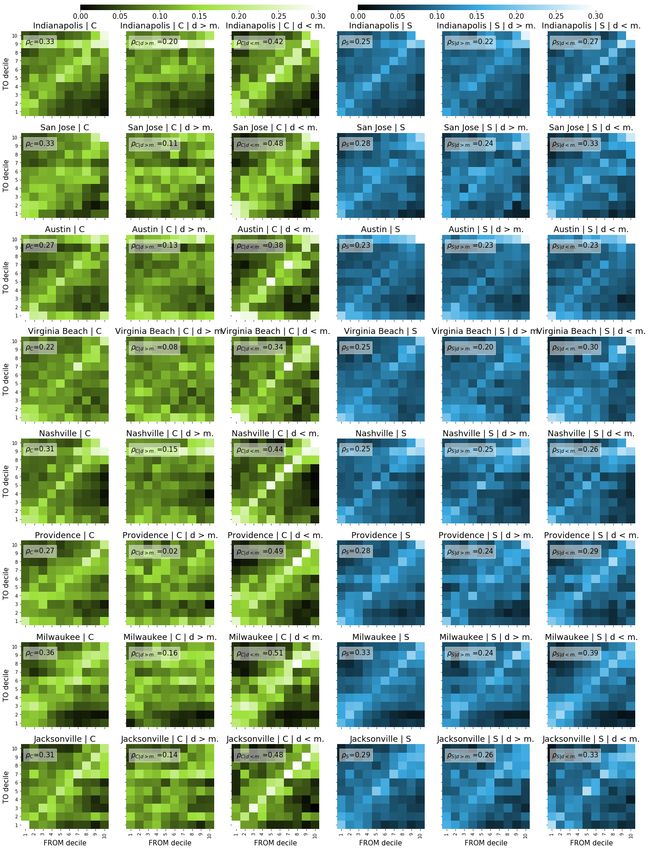
network indicators between people commuting to different distances, we find that long commuting is
associated with lower levels of transitivity, the tendency that friends of friends know each other, and
higher levels of income diversity among friends. These results are consistent across the 50 largest
US cities and suggest that long commutes can indeed facilitate social mixing.
    Our results suggest a universal role of commuting in integrating disparate social networks.
The paper contributes to the discussion on the importance of commuting in cities and shows that
longer commutes have a measurable even though moderate influence on establishing diverse and
less segregated social connections. The findings imply that supporting access to distant work can
help the inclusion of lowest income groups and to a certain degree the richest as well, regardless of
the urban context.

2    Results
We use a unique Twitter database that contains all messages and profile information of 348,850
Twitter users in the top 50 metropolitan areas of the United States. The data was collected
between 2012 and 2015 and due to the sample selection method described in Dobos et al. 2013, the
database contains a considerable amount of individuals who allowed automatic GPS data collection
for all their messages. This dataset was used in previous research to detect dominant language use
and temporal patterns connected to socio-economic indicators such as ethnicity or unemployment
in the US, to establish world-wide communities of users reflecting political and cultural boundaries,
and to model the spreading of viral content (Bokányi, Kondor, et al. 2016; Kallus, Barankai, et al.
2015; Kallus, Kondor, et al. 2017; Bokányi, Lábszki, and Vattay 2017).
    Figure 1 illustrates how commuting and social network information is retrieved from the data.
Home and work locations are detected by the most frequent locations of tweets in the morning
and evening hours or during daytime as depicted in Figure 1a (and as explained in Materials and
Methods). This process enables us to identify the census tract of home and work locations and
attach socio-economic status, measured by the average household income of census tracts from the
2012 American Community Survey. Commuting is characterized by the Euclidean distance between
home and work and the socio-economic status of both locations. Finally, we construct the ego
network for every user from mutual followership of Twitter profiles and characterize egos and alters
by the socio-economic status of their home location. This enables us to quantify social mixing in
terms of commuting and social ties in cities.
    Figure 1b shows the census tracts of inner Boston colored by the average annual household
incomes and the home and work locations of a sample user. The user’s ego network is depicted in
panel (c), with colors indicating the income of the neighbors inferred from their home census tract.
Each user in our sample has at least 1 mutual followership-based connection and has identifiable
home and work locations that are at least 100 metres away from each other. The distribution of
users across the 50 selected cities is illustrated in Supplementary Information (SI) 1 and 2. For a
more detailed description, see Materials and Methods.

                                                  3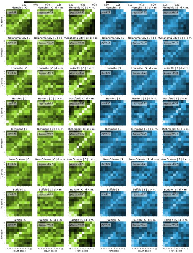
Figure 1: Combination of spatial, temporal and social network data of geolocated Twitter messages. (a) Home and
work locations of users are identified through the distribution of timestamps on all their collected tweets within their
most frequently visited spatial clusters. We assign a possible home location (8PM-8AM) and a possible work location
(9AM-5PM) to each user (Lambiotte et al. 2008; McNeill, Bright, and Hale 2017) as their most frequently visited
location in the given period. The histogram represents the timeline of tweets for the clusters of a sample user. (b)
Commuting is defined as the overhead distance between users’ home and work locations. The colorbar of the map
indicates the income level of census tracts. (c) Twitter ego network of a sample user based on mutual followership.
The coloring of nodes also corresponds to the level of income in the home tract of users.

    To characterize the relation between d, the distance of commutes, and the social network of
individuals, we compare the social networks of people commuting to d > median with d < median
commuting distances in each of the 50 largest US metropolitan areas. Median commuting distances
are calculated on the basis of the sampled users in each city as illustrated in SI 3. Our expectation is
that commuting may induce more out-of-community independent social ties for commuters, in turn
decreasing the transitivity of their egocentric networks. We observe this effect by measuring the local
clustering coefficient (Watts and Strogatz 1998) for each user, which quantifies the tendency that an
individuals’ friends know each other. Another assumption of ours is that these out-of-community
ties introduce stronger diversity in ego networks in terms of socioeconomic status of neighbors. We
quantify this effect via the average income difference from friends in users’ ego networks, which
measures the income similarity of online social connections (for a formal definition see Eq. 1 in
Materials and Methods).
    Figure 2a reports the average of local clustering coefficient and (b) the average income differences
of users commuting above and below the local median distance in the 50 largest metropolitan areas
in the USA. These findings suggest that, with a few exceptions, an above-median distance commute
is associated with lower local clustering (Figure 2a), and with greater income difference in the
commuters’ ego networks (Figure 2b). This implies that working further away from home helps
people to develop less cohesive and income-wise more diverse social networks in most metro areas.
Note that here metropolitan areas are sorted in decreasing population order and non-transparent
markers denote significant differences (p < 0.05) between averages.

                                                           4
Figure 2: Network characteristics of users and commuting distance in the top 50 metropolitan areas of the United
States. (a) Network closure measured by the local clustering coefficient is lower in most cities for those users who
commute further than the local median distance. (b) Income mixture, measured by average income difference from
friends, is higher of those who commute above the local median distance in the majority of metropolitan areas.
Non-transparent symbols indicate that the differences of means are significant (p
Similarly, elements of the social network assortativity matrix Sij represent the average probability
that a person living in a tract with income decile i has a mutual followership tie with a user living
in a tract with income decile j. For more details on the construction of the matrices, see Materials
and Methods.
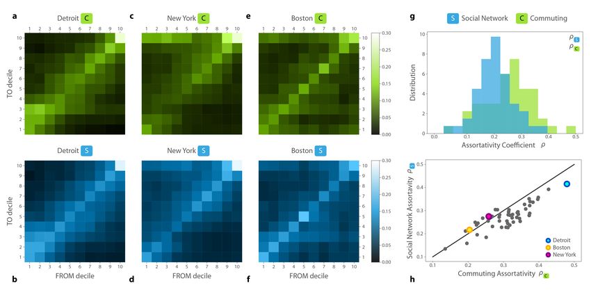
The aggregated patterns of commuting C and friendship ties S are presented in Figures 3a-f for
three example metropolitan areas, Detroit, New York, and Boston. Unlike previous studies (Dong
et al. 2020; Morales et al. 2019), we do not observe universal assortativity patterns over all cities in
these networks. In some of the cities, such as Detroit, the strong diagonal component features strong
segregation patterns, meaning that people tend to commute to neighborhoods with similar annual
household incomes as their home neighborhood, and they tend to form social ties with people living
in neighborhoods with similar income, as also found in (Heine et al. 2021). In cities like Boston,
patterns of mobility and online social ties are less assortative with higher likelihood for diverse,
off-diagonal connections. All commuting and social network matrices are available in the SI 6 for
the 50 metropolitan areas.
To explore this heterogeneity further, we computed the Pearson correlation coefficient of the
above matrices (see Materials and methods equation (4)). We use these correlation coefficients as
a single-number measure of assortativity in the metropolitan-level networks denoted by ρC for the
commuting, and ρS for the social network assortativity matrix. We show the ρC and ρS distributions
in Figure 3g. We see here that the level of assortativity varies remarkably across the 50 metro
areas, but judging by their averages, commuting in metro areas (ρ̄C = 0.31 ± 0.07) are more income
Figure 3: (a) Commuting assortativity matrix C and (b) social network assortativity matrix S between the 10
income deciles for Detroit, New York (c) and (d) and Boston (e) and (f). (h) Distribution of Pearson correlations
ρC (green) and ρS (blue) for the assortativity matrices C and S of the top 50 metropolitan areas of the US. (g)
Commuting assortativity and social network assortativity are strongly correlated across cities. Solid line represent
ρC = ρS .
6
assortative than online social ties (ρ̄S = 0.27 ± 0.05). Interestingly, our observations in Figure 3a-
f further suggest that the measured commuting and social network assortativity matrices are not
independent of each other. Indeed, Figure 3g illustrates that ρC and ρS pairs are strongly correlated
(ρ=0.84) suggesting a substantial relationship that social networks are segregated in cities where
home-work commuting patterns are assortative.
   To investigate the association between long-distance commute and social mixing on the aggregate
city-level in more detail, we separate the baseline sample of the C and S matrices by commuting
distance. Thus, we create a C and S matrix from users commuting to a distance d < median
and d > median, as in the example in Figure 4a-d, where we show these four matrices (two for
both C and S) for Detroit. These matrices indicate that for users commuting an above median
distance, matrices are less diagonal, and reflect more diverse and less segregated commuting and
social connections. Panels (e) and (f) from Figure 4 present the distributions of ρC and ρS for
the two subgroups of users in all 50 metropolitan areas. As expected, longer commuting distance
is associated with less assortativity because distant workplaces are likely to be located in socio-
economically different environments as compared to home location. This might be due to spatial
clustering of tracts with similar annual household incomes (Chodrow 2017), leading to shorter
commute patterns landing in places with similar income level. In parallel, we observe that longer
commutes are also associated with lower levels of assortativity of online social network ties such that
off-diagonal social ties are relatively more likely for d > median distances than for d < median.
However, while ρC falls sharply for d > median distances compared to d < median, the difference
of ρS is moderate in Figure 4e-f. This finding indicates that although long-distance commutes can
link disparate neighborhoods, not all of the diversity generated by commuting has imprints on social
connections. Instead, income homophily remains a major yet weaker factor of social tie selection
for long commuters as well.
   Despite the heterogeneity of metro areas, results in Figure 4g show general patterns in two re-
gards. First, assortativity of both commuting and social networks are lower for long-distance com-
muters in every metropolitan area. Second, the assortativity reduction between shorter and longer
than median commutes is decreasing sharply, while the reduction of social network assortativity is
moderate and takes similar values for every metropolitan area. The Pearson correlation coefficient
between the two assortativity values ρS and ρC is 0.80 for short commuters and 0.72 for long com-
muters, thus they signify a strong relationship between mobility and social network assortativity
patterns for both user groups (Figure 4h). To understand the magnitudes of change, we calculate the
percentage of social network assortativity reduction by ((ρS,d>median −ρS,d
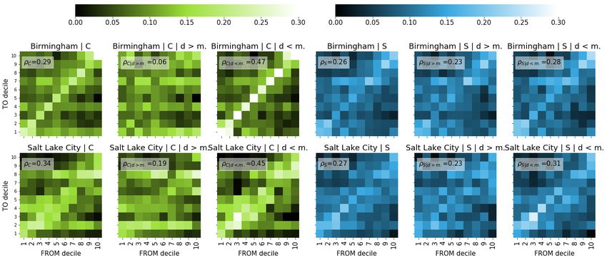
Figure 4: Panels (a)-(d) show the C and S assortativity matrices for the below (d < median) and above median
(d > median) commuting users in a selected metropolitan area, Detroit. (e)-(f) The corresponding distributions of
ρC (green) and ρS (blue) for all 50 metropolitan areas for users with d > median and d < median. (g) Pairwise
values of ρC and ρS for users with d > median and d < median by metropolitan areas. Metropolitan areas are sorted
in decreasing order by ρC for easier representation. (h) Social network assortativity versus commuting assortativity
for below and above median commuters with selected cities from Fig. 3 labeled. (i) Decrease in the commuting
assortativity and the social network assortativity measured in percentage. Black horizontal line corresponds to the
average change in social network assortativity. Grey shaded area marks the standard deviation.
                                                         8
that the uniform ∼ 30% decrease disappears if we separate two user groups randomly instead of
by commuting distance, but this observation remains consistent across multiple absolute distance
thresholds (3 km, 5 km, and 10 km). In addition, in SI 8, we show that assortativity reduction
by long-distance commute is a result of increasing social mixing of users from poorest and to some
extent, from the richest neighborhoods.
3 Discussion
Understanding the complex behavioral patterns of people is crucial to develop more liveable, equal
and sustainable urban environments. Our study contributes to this challenge by using large-scale
geolocated Twitter data to study the role of commuting in the composition and assortativity of
social interaction. We illustrate that long-distance commuting acts against structural closure and
income homophily of social relationships and reduces segregation between remote income classes by
facilitating connections and mixing. We show that home-work commutes and online social ties are
not equally assortative in every metropolitan area, but in most cases, commuting is even more likely
to point to places with similar income level than online social connections. Our findings suggest that
longer commutes are more likely to connect places with different income levels, which contributes
to the development of more diverse and less assortative social ties. Moreover, working further away
from home results in more heterogeneous social connections in every metropolitan area.
Our results suggest that urban mobility has a fundamental role in fulfilling the promise of social
inclusion and reduction of social segregation in cities. The association between commuting distance
and social networks is remarkably stable across all metropolitan areas with different size and spatial
structure (Boeing 2019). This universal pattern highlights that commuting-enabled social mixing
follows similar mechanisms regardless of the urban context. We find that facilitating the access
between distant neighborhoods can reduce segregation in metropolitan areas, while gains in social
inclusion are limited to a 30% reduction of assortativity. These results signal that providing access
across disparate neighborhoods cannot erase mechanisms of social network segregation but can
mitigate the divide between rich and poor.
The methodology applied in this paper could easily be extended to other cities with large popu-
lations of geolocated Twitter users, and where granular census data with similar spatial resolution
is available. However, this approach is not without limitations. While we are confident in our ap-
proach to identify home and work locations of users, we cannot confirm whether the identified work
locations are actual workplaces or any another facility that people visit frequently during daytime
(such as restaurants, schools, etc.). We measure commuting distances as the Euclidean distance
between the home location and the work location, whereas in multiple cities, physical obstacles
such as rivers might considerably increase to travel times or change the socio-economic segregation
patterns of settlements (Tóth, Wachs, Di Clemente, et al. 2021). We are not aware of the available
modalities to reach work destinations, but we admit that it would also introduce a large variability
into travel times. We choose this simplification because both travel times with a car or public
9transportation might depend on the exact time of the day and varying traffic conditions. Both the
underestimation of commuting distances and the inclusion of users who might not have a regular
workplace can result that the observed commuting in our case (see SI Figure 3) falls behind the
commuting distances reported in the American Community Survey. Because we do not use an ab-
solute threshold to distinguish long and short commutes, and we use the city-wise median to divide
the users into categories, we believe that the aforementioned biases do not affect our results dras-
tically. However, we test both the results of Figure 2 and Figure 4i for different absolute distance
thresholds, 3 km, 5 km and 10 km, where our results still hold (see SI 4 and SI 7).
Even though the fraction of users present in the analysis is proportional to the population
size of the 50 metropolitan areas (see SI Figure 2), we have to highlight that our dataset is not
representative for the US population and results have to be interpreted accordingly. Hargittai and
Litt 2011 finds that African American users are overrepresented on the platform, and Twitter users
are predominantly young, well-educated (Webster 2010; Sloan et al. 2015) and unrepresentative
of other ethnicities (Mislove et al. 2011; Malik et al. 2015). Therefore, we cannot generalize our
findings to the whole population of these metropolitan areas. Another limitation of the study could
be that the free 1% sample from Twitter Streaming API was used for the initial data collection.
Joseph, Landwehr, and Carley 2014; Morstatter, Pfeffer, and Liu 2014 confirms that tweets filtered
to containing GPS coordinates are retrieved to almost 90% of the time compared to the full dataset.
By imposing strict count limits, spatio-temporal constraints and mutual followership for ties, we
believe that our sample is less distorted from bot activity than what Pfeffer, Mayer, and Morstatter
2018 would suggest.
Despite the imperfection of the data, we believe that the presented exercise offers useful insights
to the structure of social connections within urban areas. Such large-scale, micro-level analysis
enables us to uncover the fundamental patterns behind segregation, inequality or the lack of inclusion
inside cities. Publicly available online social network data can complementing official census reports
or surveys and can provide opportunities to detect and react to societal patterns and changes.
4 Materials and methods
4.1 Data collection and combination methods
We focus on users of the online social networking site of Twitter who posted tweets frequently
containing precise geographic information. More specifically, we use a unique, historical database
rich in tweets containing GPS coordinates (Dobos et al. 2013; Kondor et al. 2014). These tweets
originate from users who enabled the exact geolocation option on their smartphones. Overall,
we detect the three most frequent tweeting locations of users as spatial clusters of their locations
in the 50 most populated metropolitan areas of the United States. We use the Friend-of-Friend
algorithm (Huchra and Geller 1982) to cluster the spatial coordinates for each user. This algorithm
is a paralellizable, scalable clustering algorithm known from astronomy, and it is widely used to
identify galaxy clusters (Kwon et al. 2010). In our case, any two tweet coordinates of the same
10person are considered to belong to the same spatial cluster if their separation is less than 1 km. For
each cluster, we determine the first two moments of the coordinate distribution. Before calculating
the mean coordinates of the cluster, we trim data points until all points are inside a 3σ radius to
eliminate outliers. We keep the aforementioned three highest cardinality clusters per user (Dobos
et al. 2013; Kallus, Barankai, et al. 2015).
To determine the possible home and work locations of users, we follow the approach proposed by
McNeill, Bright, and Hale 2017. We assume that the home and work locations of users are within the
previously detected three clusters. We select users for whom at least two out of the three clusters
are within the same metropolitan area from the top 50 metropolitan areas of the United States
and one of these clusters is their top cardinality location. First, we calculate the daily timeline of
clusters for each user based on the timestamp of the tweets with hourly aggregation, converting all
UTC tweet timestamps to local times across the whole US. We only consider users with more than
15 tweets on weekdays (Monday to Friday) in total. Local aggregated weekday timelines of two
clusters for a sample user are presented in Figure 1a. We calculate the share of tweets sent between
9AM and 5PM on weekdays to capture messages predominantly sent during the working hours.
Similarly, we calculate the share of tweets sent between 8PM and 8AM on weekdays contributing
to a possible home tweeting fraction. Then, the cluster with the highest work tweet share or home
tweet share becomes the work and home cluster of the user.
Commuting of users is characterized by the overhead distance between their home and work
locations. We restricted our sample to users with at least 0.1 km commutes. Thus, we have 975,492
users in our sample. The distribution of observed commuting distances for each metro area are
presented in SI 3. Additionally, we attach socio-economic data to each home and work location in
the observed metropolitan areas from the 2012 American Community Survey. More precisely, we
map the home locations of users into the census tracts of the top 50 US metropolitan areas and
attribute the average annual household income of the census tract to each user living there. After
that, we sort users into city-wise income deciles based on the average annual household incomes,
and we apply the same approach to determine the average income and the income decile of their
workplaces. Figure 1b shows the commute of the same sample user and the income level of the
surrounding census tracts.
Social connections of users are defined as their mutual followership relations on Twitter as they
represent relative stronger ties in context of online social networks (Szüle et al. 2014). Figure 1c
represents a sample ego network that we construct for every user from our home-work sample who
has at least 1 mutual followership tie within the same metropolitan area. In the end, we have 348,850
users for whom we have both the home and work location information, and a mutual followership
ego network. The composition and spatial distribution of our final sample is presented in SI 1.
Through the home location of the user’s friends, we can infer their income, thus, we are able to
characterize the socio-economic status of the neighbors in the ego networks by identifying their
income deciles. Figure 1c shows this characterization by using the same colorscale for both the ego
and its first neighbors as the choropleth map in Figure 1b.
11At the individual level, commuting and online social ties of our users are characterized by
multiple different indicators. We measure user commutes by the Euclidean distance d between their
inferred home and work locations. We calculate degree and local clustering coefficient from their
ego networks. We also measure the average income difference between their own home income and
the home income of their friends, following the formula below:
1 X
∆I = log10 |If − Iego | (1)
#neighbors
f ∈neighbors
4.2 Assortativity metrics
At the aggregated, metropolitan area level, we create multiple different assortativity matrices be-
tween income deciles D for each metropolitan area. First, an assortativity matrix of commuting is
constructed, where we capture the probability Cij that a user u belonging to a home census tract
in income decile D = i commutes to a tract with income decile D = j to work. Second, we measure
the conditional probabilities of social ties across home census tracts in different income deciles, the
social network assortativity matrix S. The element Sij of this matrix measures the probability that
a user u from income decile D = i has a mutual followership tie to a user in income decile D = j.
Formally, the two matrices can be calculated as
P
1
{u∈U |Du,home=j ,Du,work=i }
Cij = P (2)
1
{u∈U |Du,home=j }
P 1 P
ku 1
{u∈U |Du,home =j } {euf ∈Eu |Df,home=i }
Sij = P , (3)
1
{u∈U |Du,home=j }
where U is the user set within a metropolitan area for which we calculate the matrices, Eu is the
set of edges connected to the user u, ku is the degree of ego user u in the ego network, eu f is the
undirected edge between user u and f , Du and Df are the (home or work) deciles of users u and
f , respectively. We also measure two additional friendship and commuting assortativity matrices,
S d>median , S dmedian and C dWe measure assortativity in these matrices by calculating the Pearson correlation coefficient ρ
of the matrix entries. If we normalize the elements of matrix X such that X̃ij = Xij /n, where
P
n = i,j Xij , the sum of the elements of a matrix, then ρ captures how diagonal these matrices are:
P P P
ij X̃ij − iX̃ij j X̃ij
i,j i,j i,j
ρX = v !2 v !2 , (4)
u u
uP uP
i2 X̃ij − iX̃ij t j 2 X̃ij −
P P
t j X̃ij
i,j i,j i,j i,j
where the summation for i and j both go over all of the income deciles D = 1, . . . , 10. An as-
sortativity value ρ = +1 would mean a completely diagonal, thus, completely assortative matrix,
whereas ρ ≈ 0 values indicate the lack of any preference for people following others from the very
same income class of their own.
13References
[1] Jane Jacobs. The death and life of great American cities. Vintage, 2016.
[2] Edward Glaeser. “Cities, productivity, and quality of life”. In: Science 333.6042 (2011),
pp. 592–594.
[3] Luı́s M A Bettencourt. “The Origins of Scaling in Cities”. In: Science 340.6139 (June 2013),
pp. 1438–1441. doi: 10.1126/science.1235823.
[4] Gilles Duranton and Diego Puga. “The economics of urban density”. In: Journal of Economic
Perspectives 34.3 (2020), pp. 3–26. doi: 10.1257/jep.34.3.3.
[5] Michael Storper and Anthony J Venables. “Buzz: Face-to-face contact and the urban econ-
omy”. In: Journal of Economic Geography 4.4 (2004), pp. 351–370. doi: 10.1093/jnlecg/
lbh027.
[6] Francesco Calabrese et al. “Interplay between telecommunications and face-to-face interac-
tions: A study using mobile phone data”. In: PLoS ONE 6.7 (2011), e20814. doi: 10.1371/
journal.pone.0020814.
[7] Shi Kai Chong et al. “Economic outcomes predicted by diversity in cities”. In: EPJ Data
Science 9.1 (2020), p. 17. doi: 10.1140/epjds/s13688-020-00234-x.
[8] Robert J. Sampson. “Moving to Inequality: Neighborhood Effects and Experiments Meet
Social Structure”. In: American Journal of Sociology 114.1 (July 2008), pp. 189–231. doi:
10.1086/589843.
[9] Edward L Glaeser, Matt Resseger, and Kristina Tobio. “Inequality in cities”. In: Journal of
Regional Science 49.4 (2009), pp. 617–646. doi: 10.1111/j.1467-9787.2009.00627.x.
[10] Richard Florida and Charlotta Mellander. “Segregated city: The geography of economic seg-
regation in America’s metros”. In: Martin Prosperity Institute (2015).
[11] Elizabeth Oltmans Ananat. “The wrong side(s) of the tracks: The causal effects of racial segre-
gation on urban poverty and inequality”. In: American Economic Journal: Applied Economics
3.2 (2011), pp. 34–66. doi: 10.1257/app.3.2.34.
[12] Philip S Chodrow. “Structure and information in spatial segregation”. In: Proceedings of the
National Academy of Sciences of the United States of America 114.44 (2017), pp. 11591–
11596. doi: 10.1073/pnas.1708201114.
[13] Richard Fry and Paul Taylor. “The rise of residential segregation by income”. In: Pew Research
Center (2012).
[14] Eszter Bokányi, Dániel Kondor, et al. “Race, religion and the city: twitter word frequency
patterns reveal dominant demographic dimensions in the United States”. In: Palgrave Com-
munications 2.1 (Dec. 2016), p. 16010. doi: 10.1057/palcomms.2016.10.
[15] Douglas S Massey and Nancy A Denton. “The dimension of residential segregation”. In: Social
Forces 67.2 (1988), pp. 281–315.
14[16] Nathan Eagle, Alex Pentland, and David Lazer. “Inferring friendship network structure by
using mobile phone data”. In: Proceedings of the National Academy of Sciences of the United
States of America 106.36 (2009), pp. 15274–15278. doi: 10.1073/pnas.0900282106.
[17] Michael Bailey et al. “Social connectedness in urban areas”. In: Journal of Urban Economics
118 (July 2020), p. 103264. doi: 10.1016/j.jue.2020.103264.
[18] Lukas Norbutas and Rense Corten. “Network structure and economic prosperity in municipal-
ities: A large-scale test of social capital theory using social media data”. In: Social Networks
52 (Jan. 2018), pp. 120–134. doi: 10.1016/j.socnet.2017.06.002.
[19] Jacob Levy Abitbol and Marton Karsai. “Interpretable socioeconomic status inference from
aerial imagery through urban patterns”. In: Nature Machine Intelligence 2.11 (2020), pp. 684–
692.
[20] Gergő Tóth, Johannes Wachs, Riccardo Di Clemente, et al. “Inequality is rising where social
network segregation interacts with urban topology”. In: arXiv 12.1 (2019), pp. 1–9. doi:
10.1038/s41467-021-21465-0.
[21] Qi Wang et al. “Urban mobility and neighborhood isolation in America’s 50 largest cities”.
In: Proceedings of the National Academy of Sciences 115.30 (July 2018), pp. 7735–7740. doi:
10.1073/pnas.1802537115.
[22] Luca Pappalardo et al. “Using big data to study the link between human mobility and socio-
economic development”. In: Proceedings - 2015 IEEE International Conference on Big Data,
IEEE Big Data 2015. IEEE. 2015, pp. 871–878. doi: 10.1109/BigData.2015.7363835.
[23] Xiaowen Dong et al. “Segregated interactions in urban and online space”. In: EPJ Data
Science 9.1 (Dec. 2020), p. 20. doi: 10.1140/epjds/s13688-020-00238-7.
[24] Cate Heine et al. “Analysis of mobility homophily in Stockholm based on social network data”.
In: PLoS ONE 16.3 March (2021), pp. 1–14. doi: 10.1371/journal.pone.0247996.
[25] Nathan Eagle, Michael Macy, and Rob Claxton. “Network diversity and economic develop-
ment”. In: Science 328.5981 (2010), pp. 1029–1031. doi: 10.1126/science.1186605.
[26] Shan Jiang et al. “The TimeGeo modeling framework for urban motility without travel sur-
veys”. In: Proceedings of the National Academy of Sciences of the United States of America
113.37 (2016), E5370–E5378. doi: 10.1073/pnas.1524261113.
[27] Eric Dahlin, Erin Kelly, and Phyllis Moen. “Is work the new neighborhood? Social ties in the
workplace, family, and neighborhood”. In: Sociological Quarterly 49.4 (2008), pp. 719–736.
doi: 10.1111/j.1533-8525.2008.00133.x.
[28] Francesco Calabrese et al. “Interplay between Telecommunications and Face-to-Face Interac-
tions: A Study Using Mobile Phone Data”. In: PLoS ONE 6.7 (July 2011). Ed. by Enrico
Scalas, e20814. doi: 10.1371/journal.pone.0020814.
15[29] Mario L. Small and Laura Adler. “The Role of Space in the Formation of Social Ties”. In:
Annual Review of Sociology 45 (2019), pp. 111–132. doi: 10.1146/annurev- soc- 073018-
022707.
[30] Gil Viry. “Residential mobility and the spatial dispersion of personal networks: Effects on
social support”. In: Social Networks 34.1 (Jan. 2012), pp. 59–72. doi: 10.1016/j.socnet.
2011.07.003.
[31] Joshua Blumenstock, Guanghua Chi, and Xu Tan. “Migration and the Value of Social Net-
works”. 2019.
[32] Elizabeth Roberto. “The Spatial Proximity and Connectivity Method for Measuring and An-
alyzing Residential Segregation”. In: Sociological Methodology 48.1 (2018), pp. 182–224. doi:
10.1177/0081175018796871.
[33] Maarten van Ham, Tiit Tammaru, and Heleen J Janssen. “A multi-level model of vicious
circles of socio-economic segregation”. In: Divided Cities. Vol. 615159. 8774. OECD, 2018,
pp. 135–153. doi: 10.1787/9789264300385-8-en.
[34] Jaap Nieuwenhuis et al. “Does segregation reduce socio-spatial mobility? Evidence from four
European countries with different inequality and segregation contexts”. In: Urban Studies 57.1
(Jan. 2020), pp. 176–197. doi: 10.1177/0042098018807628.
[35] Alfredo J. Morales et al. “Segregation and polarization in urban areas”. In: Royal Society
Open Science 6.10 (Oct. 2019), p. 190573. doi: 10.1098/rsos.190573.
[36] Manuel A Florez et al. “Measuring the impacts of economic well being in commuting networks
— A case study of Columbia”. In: Transportation Research Board, 96th Annual Meeting.
Vol. 17. 03745. 2016.
[37] Teodoro Dannemann, Boris Sotomayor-Gómez, and Horacio Samaniego. “The time geogra-
phy of segregation during working hours”. In: Royal Society Open Science 5.10 (Oct. 2018),
p. 180749. doi: 10.1098/rsos.180749.
[38] Nibir Bora, Yu-Han Chang, and Rajiv Maheswaran. “Mobility Patterns and User Dynamics in
Racially Segregated Geographies of US Cities”. In: Proceedings of the international conference
on social computing, behavioral-cultural modeling, and prediction (2014), pp. 11–18. doi: 10.
1007/978-3-319-05579-4_2.
[39] Yannick Leo et al. “Socioeconomic correlations and stratification in social-communication
networks”. In: Journal of The Royal Society Interface 13.125 (Dec. 2016), p. 20160598. doi:
10.1098/rsif.2016.0598.
[40] Ngai Ming Yip, Ray Forrest, and Shi Xian. “Exploring segregation and mobilities: Application
of an activity tracking app on mobile phone”. In: Cities 59 (2016), pp. 156–163. doi: 10.1016/
j.cities.2016.02.003.
16[41] Laszlo Dobos et al. “A multi-terabyte relational database for geo-tagged social network data”.
In: 2013 IEEE 4th International Conference on Cognitive Infocommunications (CogInfoCom).
IEEE, Dec. 2013, pp. 289–294. doi: 10.1109/CogInfoCom.2013.6719259.
[42] Zsófia Kallus, Norbert Barankai, et al. “Spatial Fingerprints of Community Structure in Hu-
man Interaction Network for an Extensive Set of Large-Scale Regions”. In: PLOS ONE 10.5
(May 2015). Ed. by Bin Jiang, e0126713. doi: 10.1371/journal.pone.0126713.
[43] Zsófia Kallus, Dániel Kondor, et al. “Video Pandemics: Worldwide Viral Spreading of Psy’s
Gangnam Style Video”. In: ICT Innovations 2017: Data-Driven Innovation. Ed. by Dimitar
Trajanov and Verica Bakeva. Vol. 778. Cham: Springer International Publishing, 2017, pp. 3–
12. doi: 10.1007/978-3-319-67597-8_1.
[44] Eszter Bokányi, Zoltán Lábszki, and Gábor Vattay. “Prediction of employment and unem-
ployment rates from Twitter daily rhythms in the US”. In: EPJ Data Science 6.1 (Dec. 2017),
p. 14. doi: 10.1140/epjds/s13688-017-0112-x.
[45] Renaud Lambiotte et al. “Geographical dispersal of mobile communication networks”. In:
Physica A: Statistical Mechanics and its Applications 387.21 (Sept. 2008), pp. 5317–5325.
doi: 10.1016/j.physa.2008.05.014.
[46] Graham McNeill, Jonathan Bright, and Scott A. Hale. “Estimating local commuting patterns
from geolocated Twitter data”. In: EPJ Data Science 6.1 (Dec. 2017), p. 24. doi: 10.1140/
epjds/s13688-017-0120-x.
[47] Duncan J. Watts and Steven H. Strogatz. “Collective dynamics of ’small-world9 networks”.
In: Nature 393.6684 (June 1998), pp. 440–442. doi: 10.1038/30918.
[48] Geoff Boeing. “Urban spatial order: street network orientation, configuration, and entropy”.
In: Applied Network Science 4.1 (Dec. 2019), p. 67. doi: 10.1007/s41109-019-0189-1.
[49] Gergő Tóth, Johannes Wachs, Riccardo Di Clemente, et al. “Inequality is rising where social
network segregation interacts with urban topology”. In: Nature Communications 12.1 (Dec.
2021), p. 1143. doi: 10.1038/s41467-021-21465-0.
[50] Eszter Hargittai and Eden Litt. “The tweet smell of celebrity success: Explaining variation
in Twitter adoption among a diverse group of young adults”. In: New Media & Society 13.5
(Aug. 2011), pp. 824–842. doi: 10.1177/1461444811405805.
[51] Tom Webster. “Twitter Usage In America : 2010”. In: Edison Research/ Arbitron Internet
and Multimedia Study. (2010).
[52] Luke Sloan et al. “Who Tweets? Deriving the Demographic Characteristics of Age, Occupation
and Social Class from Twitter User Meta-Data”. In: PLOS ONE 10.3 (Mar. 2015). Ed. by
Tobias Preis, e0115545. doi: 10.1371/journal.pone.0115545.
[53] Alan Mislove et al. “Understanding the Demographics of Twitter Users”. In: Int’l AAAI
Conference on Weblogs and Social Media (ICWSM). 2011, pp. 554–557.
17[54] Momin M Malik et al. “Population bias in geotagged tweets”. In: AAAI Workshop - Technical
Report WS-15-18 (2015), pp. 18–27.
[55] Kenneth Joseph, Peter M. Landwehr, and Kathleen M. Carley. “Two 1%s Don’t Make a
Whole: Comparing Simultaneous Samples from Twitter’s Streaming API”. In: Association fo
the Advanced of Artificial Intelligence. June 2014, pp. 75–83. doi: 10 . 1007 / 978 - 3 - 319 -
05579-4_10.
[56] Fred Morstatter, Jürgen Pfeffer, and Huan Liu. “When is it biased?” In: Proceedings of the
23rd International Conference on World Wide Web - WWW ’14 Companion. New York, New
York, USA: ACM Press, Jan. 2014, pp. 555–556. doi: 10.1145/2567948.2576952.
[57] Jürgen Pfeffer, Katja Mayer, and Fred Morstatter. “Tampering with Twitter’s Sample API”.
In: EPJ Data Science 7.1 (Dec. 2018), p. 50. doi: 10.1140/epjds/s13688-018-0178-0.
[58] Dániel Kondor et al. “Efficient classification of billions of points into complex geographic re-
gions using hierarchical triangular mesh”. In: Proceedings of the 26th International Conference
on Scientific and Statistical Database Management - SSDBM ’14. New York, New York, USA:
ACM Press, 2014, pp. 1–4. doi: 10.1145/2618243.2618245.
[59] J P Huchra and M. J. Geller. “Groups of galaxies. I - Nearby groups”. In: The Astrophysical
Journal 257 (June 1982), p. 423. doi: 10.1086/160000.
[60] Yongchul Kwon et al. “Scalable clustering algorithm for N-body simulations in a shared-
nothing cluster”. In: Lecture Notes in Computer Science (including subseries Lecture Notes in
Artificial Intelligence and Lecture Notes in Bioinformatics) 6187 LNCS (2010), pp. 132–150.
doi: 10.1007/978-3-642-13818-8_11.
[61] János Szüle et al. “Lost in the City: Revisiting Milgram’s Experiment in the Age of Social
Networks”. In: PLoS ONE 9.11 (Nov. 2014). Ed. by Jordi Garcia-Ojalvo, e111973. doi: 10.
1371/journal.pone.0111973.
185 Acknowledgements
Eszter Bokányi was supported by the ÚNKP-20-4 New National Excellence Program of the Min-
istry for Innovation and Technology from the source of the National Research, Development and
Innovation Fund of Hungary. Márton Karsai acknowledges support from the H2020 SoBigData++
project (H2020-871042) and the DataRedux ANR project (ANR-19-CE46-0008). Balázs Lengyel
and Sándor Juhász acknowledge support from the Hungarian Scientific Research Fund (OTKA K-
129207). We thank for the usage of ELKH Cloud (https://science-cloud.hu/) that significantly
helped us achieving the results published in this paper. We thank József Stéger for helping in the
maintenance of the Twitter database, and Szabolcs Tóth-Zs. (https://bandart.eu/) for figure
design.
19Supplementary information
SI 1: Observed users across the top 50 US metropolitan areas
Figure 5: (A) Map of the selected 50 metropolitan areas with the highest population in the US. (B) The histogram
represents the number of observed users with home and work locations, minimum 100 meter commute and minimum
1 connection to a user with discovered home and work locations in the same metro area. The metro areas are ordered
by population.
20SI 2: Population and observed users in metro areas
Figure 6: Population size and observed users in the selected 50 metropolitan areas of the US. Observed users
have detected home and work locations, commute at least 100 meter and have at least 1 friendship tie to users with
discovered home and work locations inside the same metro area.
SI 3: Distribution of commuting distances
Figure 7: The distribution of commuting distances in the selected 50 metropolitan areas represented by boxplots.
Black dots represent the average commuting distance in each metro area in our data. We only consider those users
for whom home and work locations are identifiable, home and work is separated by a minimum 100 meter commute,
and the user has minimum 1 friend with identified home and work locations in the same metro area. The metro areas
are ordered by population and outlier individuals are not presented.
21SI 4: Effect of different distance thresholds
Figure 8: Network characteristics of users commuting above and below 3 km distance in the top 50 metropolitan
areas of the United States. The slightly more transparent signs indicate that differences of means are not significant
(p>0.05).
22Figure 9: Network characteristics of users commuting above or below 5 km distance in the top 50 metropolitan
areas of the United States. The slightly more transparent signs indicate that differences of means are not significant
(p>0.05).
23Figure 10: Network characteristics of users commuting above or below 10 km distance in the top 50 metropolitan
areas of the United States. The slightly more transparent signs indicate that differences of means are not significant
(p>0.05).
24SI 5: Regression on network characteristics and commuting
Table 1 presents 8 linear regression models to complement Figure 2 of the main text. For these
robustness checks we log transferred (indicated in the table) or normalized the variables. We
introduce control variables step-by-step. Model (1)-(4) further strengthens our previous findings at
Figure 2a as longer commuting is connected to lower local clustering in the mutual followership ego
network of users. However, the positive and significant quadratic term suggests that commuting
distance has an increasing return on network clustering. This relationship is stable even while
controlling for the degree, home income and metro area of users. Model (5) shows that longer
commutes are linked to ego networks with lower income difference between friends and commuting
distance has a diminishing return on income difference to friends. However, this relationship does
not hold while controlling for the degree and home income of users in Model (8) whereas controllers
introduced in Models (6)-(7) are stable.
Table 1: Relationship between commuting and network characteristics
Dependent variable
Local clustering Income diff. (log)
(1) (2) (3) (4) (5) (6) (7) (8)
∗∗∗ ∗∗∗ ∗∗
Distance (log) −0.056 −0.036 0.078 −0.035
(0.003) (0.003) (0.031) (0.028)
Distance2 (log) 0.023∗∗∗ 0.013∗∗∗ −0.059∗∗∗ 0.008
(0.002) (0.001) (0.016) (0.014)
Degree (log) −0.178∗∗∗ −0.179∗∗∗ 0.368∗∗∗ 0.422∗∗∗
(0.001) (0.001) (0.005) (0.005)
Income (log) 0.018∗∗∗ −0.003∗∗ 3.506∗∗∗ 3.546∗∗∗
(0.001) (0.001) (0.013) (0.013)
Constant 0.155∗∗∗ 0.369∗∗∗ 0.049∗∗∗ 0.404∗∗∗ 1.049∗∗∗ 0.651∗∗∗ −14.394∗∗∗ −15.014∗∗∗
(0.002) (0.002) (0.007) (0.006) (0.020) (0.016) (0.059) (0.060)
Metro FE Yes Yes Yes Yes Yes Yes Yes Yes
Observations 261,283 261,283 258,949 258,949 348,728 348,728 345,610 345,610
R2 0.009 0.243 0.007 0.244 0.009 0.023 0.182 0.200
Adjusted R2 0.008 0.243 0.007 0.244 0.009 0.023 0.182 0.200
∗ ∗∗ ∗∗∗
Note: pTable 2 presents 3 additional linear regression models to uncover the relationship between the degree
of users and their commuting distance. Results are in line with the trends of SI 4 Figure 8-10 as
longer commuting is connected to higher degree, however, commuting distance has diminishing
returns on user degree.
Table 2: Relationship between degree and commuting
Dependent variable
Degree
(1) (2) (3)
∗∗∗
Distance (log) 0.146 0.144∗∗∗
(0.010) (0.010)
Distance2 (log) −0.074∗∗∗ −0.073∗∗∗
(0.005) (0.005)
Income (log) −0.096∗∗∗ −0.096∗∗∗
(0.005) (0.005)
Constant 1.047∗∗∗ 1.528∗∗∗ 1.474∗∗∗
(0.007) (0.021) (0.021)
Metro FE Yes Yes Yes
Observations 348,728 345,610 345,610
R2 0.007 0.007 0.008
Adjusted R2 0.007 0.007 0.008
∗ ∗∗ ∗∗∗
Note: pSI 6: All assortativity matrices for the top 50 US metropolitan areas
Figure 11: Assortativity matrices C and S in all 50 investigated US metropolitan areas for the overall, mobile and non-mobile users.
ρ-values are indicated in the labels.
27Figure 11: (continued) Assortativity matrices C and S in all 50 investigated US metropolitan areas for the overall, mobile and non-mobile
users. ρ-values are indicated in the labels.
28Figure 11: (continued) Assortativity matrices C and S in all 50 investigated US metropolitan areas for the overall, mobile and non-mobile
users. ρ-values are indicated in the labels.
29Figure 11: (continued) Assortativity matrices C and S in all 50 investigated US metropolitan areas for the overall, mobile and non-mobile
users. ρ-values are indicated in the labels.
30Figure 11: (continued) Assortativity matrices C and S in all 50 investigated US metropolitan areas for the overall, mobile and non-mobile
users. ρ-values are indicated in the labels.
31Figure 11: (continued) Assortativity matrices C and S in all 50 investigated US metropolitan areas for the overall, mobile and non-mobile
users. ρ-values are indicated in the labels.
32SI 7: Different distance thresholds and assortativity change
Figure 12: Change in the assortativity of the social network matrices vs. the commuting matrices
for different distance thresholds
Figure 13: Change in the assortativity of the social network matrices vs. the commuting matrices
for two random user groups
33SI 8: Diversity in commuting and social connections
We measure the diversity SC and SS of the matrices C and S (or for any matrices on the smaller
user base, e.g. Sd>median ) by averaging the normalized entropiesPof the columns of the matrices.
Formally, for a 10 × 10 matrix X, where the sum of the columns j Xij = 1 for every possible j,
10 10
1 X 1 X
SX = · Xij · log Xij , (5)
10 log 10
j=1 i=1
which means that SX = 0 corresponds to a matrix in which every column contains exactly one
element that is 1, and the others are 0, and SX = 1 corresponds to the case when every element
1
of the matrix is equal, 10 . Thus, SX values closer to 1 mean matrices in which commuting or
friendship ties in a column are on average more distributed over multiple income classes, whereas
smaller SX values mean matrix columns with rather one dominant element.
In parallel to the decreasing assortativity with longer commutes, we can observe an increasing
average diversity for the connection patterns of both matrices, if measured by the averaged entropy
of the column-wise probability distributions SS and SC (see Section 4 for details on this measure).
This increase in the diversity is shown for all 50 metropolitan areas. Again, there is a higher
increase in diversity for the commuting assortativity matrix, if we compare long commuters to
short commuters, but this increase in the diversity is in parallel with the increase in the friendship
assortativity matrix. If we measure which income deciled contribute to the increasing entropy
values in both the mobility and the social network patterns, we can see that the lowest and highest
income classes have the most diversity increase (see the inset). Therefore, it is most likely that
rearrangement of the social connections of the richest and poorest deciles contribute most to the
30% decrease in social network assortativity that comes with longer commutes.
Figure 14: Diversity
34Figure 15: Assortativity of commuting and social network matrices by income groups.
35You can also read