On the semi-annual variation of relativistic electrons in the outer radiation belt
←
→
Page content transcription
If your browser does not render page correctly, please read the page content below
Ann. Geophys., 39, 413–425, 2021
https://doi.org/10.5194/angeo-39-413-2021
© Author(s) 2021. This work is distributed under
the Creative Commons Attribution 4.0 License.

On the semi-annual variation of relativistic electrons in the outer
radiation belt
Christos Katsavrias1,2 , Constantinos Papadimitriou1,2 , Sigiava Aminalragia-Giamini1,2 , Ioannis A. Daglis1,3 ,
Ingmar Sandberg2 , and Piers Jiggens4
1 Department  of Physics, National and Kapodistrian University of Athens, Athens, Greece
2 Space Applications and Research Consultancy (SPARC), Athens, Greece
3 Hellenic Space Center, Athens, Greece
4 ESA/ESTEC, Noordwijk, the Netherlands

Correspondence: Christos Katsavrias (ckatsavrias@phys.uoa.gr)

Received: 19 December 2020 – Discussion started: 8 January 2021
Revised: 5 April 2021 – Accepted: 7 April 2021 – Published: 12 May 2021

Abstract. The nature of the semi-annual variation in the rel-      shown that the trapped relativistic electron population, in the
ativistic electron fluxes in the Earth’s outer radiation belt is   near-Earth space, can be enhanced, depleted or even not af-
investigated using Van Allen Probes (MagEIS and REPT)              fected at all due to the interplay of acceleration and loss
and Geostationary Operational Environmental Satellite En-          mechanisms (Reeves et al., 2003; Katsavrias et al., 2015;
ergetic Particle Sensor (GOES/EPS) data during solar cy-           Turner et al., 2015; Reeves and Daglis, 2016; Katsavrias et
cle 24. We perform wavelet and cross-wavelet analysis in a         al., 2019a; Daglis et al., 2019).
broad energy and spatial range of electron fluxes and exam-           Nevertheless, the relativistic electron fluxes in the outer
ine their phase relationship with the axial, equinoctial and       radiation belt also show variations on longer timescales, ex-
Russell–McPherron mechanisms. It is found that the semi-           hibiting a semi-annual as well as an annual periodicity. Even
annual variation in the relativistic electron fluxes exhibits      though this semi-annual variation (henceforward SAV) has
pronounced power in the 0.3–4.2 MeV energy range at L              long been recognized in geomagnetic activity (Cortie, 1912;
shells higher than 3.5, and, moreover, it exhibits an in-phase     Chapman and Bartels, 1940), in the electron fluxes of the
relationship with the Russell–McPherron effect, indicating         radiation belt, it was reported for the first time in Baker et
the former is primarily driven by the latter. Furthermore, the     al. (1999) using 2–6 MeV electron flux measurements from
analysis of the past three solar cycles with GOES/EPS indi-        the Solar Anomalous and Magnetospheric Particle Explorer
cates that the semi-annual variation at geosynchronous orbit       (SAMPEX) satellite. Over the past 20 years, the cause of the
is evident during the descending phases and coincides with         SAV in the relativistic electrons of the outer belt has still been
periods of a higher (lower) high-speed stream (HSS) (inter-        under debate, and three possible mechanisms have been pro-
planetary coronal mass ejection, ICME) occurrence.                 posed:

                                                                     1. the axial effect (Svalgaard, 1977), the variation of the
                                                                        position of the Earth in heliographic latitude (λ) result-
1   Introduction                                                        ing in a varying exposure of the terrestrial magneto-
                                                                        sphere to high-speed solar wind streams (e.g., coronal
The outer radiation belt consists of electrons with energies            holes);
from hundreds of kiloelectron volts (keV) to several mega-
electron volts (MeV), and its response to geospace distur-           2. the equinoctial effect (Cliver et al., 2000, 2002), that is
bances is extremely variable, spanning from a few hours to              the varying angle of the Earth’s dipole (ψ) with respect
several days or even months. Concerning the short-term (a               to the Earth–Sun line (and consequently the solar wind
few hours to a few days) variability, previous studies have             speed) with the angle at 90◦ during the equinoxes; and

Published by Copernicus Publications on behalf of the European Geosciences Union.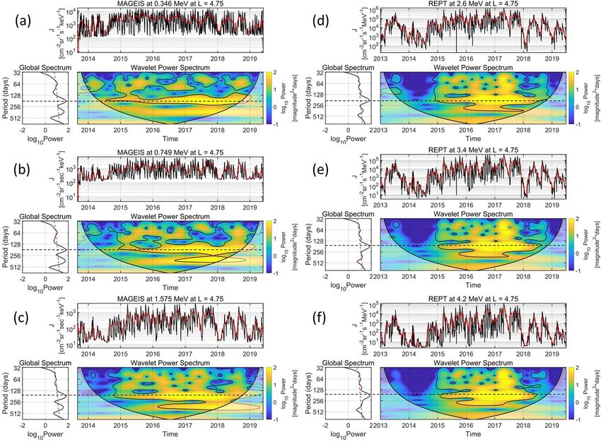
414                                                             C. Katsavrias et al.: Semi-annual variation of outer belt electrons

                                                                        southward component of the IMF plays a crucial role in de-
                                                                        termining which geomagnetic storms result in increased elec-
                                                                        tron fluxes and which do not; therefore this may account for
                                                                        the dominance of the RM effect as far as relativistic electrons
                                                                        are concerned.
                                                                           Furthermore, Emery et al. (2011) used > 2 MeV electron
                                                                        fluxes from Geostationary Operational Environmental Satel-
                                                                        lite (GOES) and argued that the SAV, which was relatively
                                                                        strong in the 1995–1997 solar minimum, was a combina-
                                                                        tion of the Russell–McPherron effect and the appearance of
                                                                        equinoctial peaks in the amplitudes of solar rotation periods
                                                                        of 13.5 and 27 d. Finally, Poblet et al. (2020) used GOES
                                                                        > 2 MeV electron fluxes during the 1987–2008 time period
                                                                        and concluded that the equinoctial mechanism seems to be
                                                                        the dominant driver of the SAV of electron fluence at GEO.
                                                                           This study aims to investigate the causes of this semi-
                                                                        annual variation by exploiting the high-resolution data of the
                                                                        Van Allen probes and by estimating its occurrence – during
Figure 1. Annual profiles of the absolute value of the λ angle gov-     solar cycle 24 (henceforward SC24) – using sophisticated
erning the axial mechanism (dotted black line), the solar declination   wavelet techniques (e.g., cross-wavelet and wavelet coher-
ψ governing the equinoctial mechanism (solid black line) and the θ      ence).
angle responsible for the Russell–McPherron effect (dashed black
line). The vertical lines correspond to the equinoxes’ maxima (red
and blue) and the summer solstice minimum (green) derived from          2     Data and methods
the three mechanisms (Cliver et al., 2002).
                                                                        2.1    Data selection and preprocessing
  3. the Russell–McPherron (henceforward RM) effect
                                                                        We use the spin-averaged differential fluxes from the Mag-
     (Russell and McPherron, 1973), an effect due to the
                                                                        netic Electron Ion Spectrometer (MagEIS; Blake et al.,
     larger z component of the interplanetary magnetic field
                                                                        2013) and the Relativistic Electron Proton Telescope (REPT;
     (IMF) near the equinoxes in GSM coordinates, which
                                                                        Baker et al., 2012) on board the Radiation Belt Storm
     results from the tilt of the dipole axis with respect to the
                                                                        Probes (RBSP). The dataset spans the time period from Jan-
     heliographic equatorial plane (θ ).
                                                                        uary 2013 until July 2019, which corresponds to the late
   The daily values of these three angles are plotted in Fig. 1         maximum and descending phase of solar cycle 24.
in a similar way to that in Cliver et al. (2002).                          Over the early part of the mission, the MagEIS instru-
   Since Baker et al. (1999), several studies have attempted            ments underwent several major changes to energy channel
to shed light on the cause of the SAV occurrence. Li et al.             definitions, operational modes and flux conversion factors.
(2001) used 8 years of SAMPEX electron flux measurements                Therefore, in this study, we will focus on data from Septem-
in the 2–6 MeV energy range and divided the SAV into two                ber 2013 onward, when the major operational changes were
parts: a semi-annual variation due to the response of the mag-          mostly complete. We use the background-corrected data
netosphere to the solar wind, such as the equinoctial effect,           (level 2; see also Claudepierre et al., 2015) using measure-
and a semi-annual variation in the solar wind itself in GSM             ments where the background correction error is less than
coordinates, such as the axial and RM effects. They argued              75 %, similar to Boyd et al. (2019). From this procedure,
that the semi-annual variation of the Dst index and megaelec-           several energy channels from both MagEIS units are ex-
tron volt (MeV) electrons deep in the inner magnetosphere               cluded due to an insufficient amount of data. REPT chan-
can be attributed mostly to the equinoctial effect (orientation         nels, especially those with higher energies (> 5 MeV), are
of the Earth’s dipole axis relative to solar wind flow), with           often dominated by background measurements induced by
the axial (heliographic latitude) and the RM (IMF z com-                contamination due to galactic cosmic rays. This results in a
ponent in GSM coordinates) effects also contributing, while             flattening of the spectrum at channels 6–12 (E > 5.3 MeV).
the semi-annual variation of MeV electrons at geostationary             For the lower energy channels, the foreground signal is al-
orbit (henceforward GEO) is attributed mostly to the semi-              ways much stronger than the background, so no correc-
annual variation of solar wind velocity as seen by Earth.               tion is needed. The instrument’s background is extracted by
A few years later, Kanekal et al. (2010) argued that while              applying a sinusoidal fit in the flux data at L > 6 (GEO)
the equinoctial mechanism may be the dominant mechanism                 following Boyd et al. (2019). Table 1 shows the nominal
for the seasonal dependence of the geomagnetic activity, the            energy values of the combined RBSP A and B channels

Ann. Geophys., 39, 413–425, 2021                                                        https://doi.org/10.5194/angeo-39-413-2021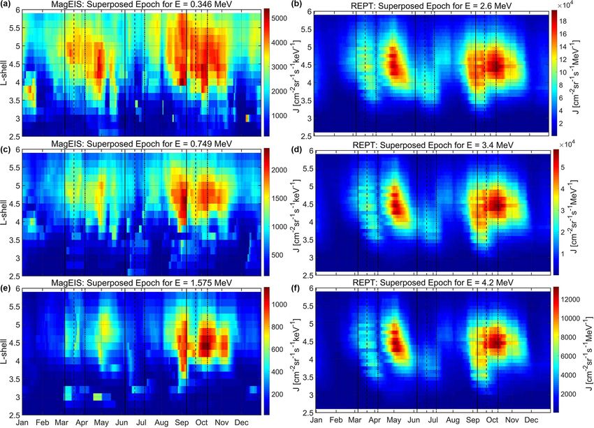
C. Katsavrias et al.: Semi-annual variation of outer belt electrons                                                                415

Table 1. MagEIS and REPT energy channels used in this study.            and scaled in time:

      Instrument                                    Energy (MeV)
                                                                                      Z∞         p
                                                                        W (t, f ) =        F (τ ) f ψ ∗ [f (τ − t)]dτ.             (1)
      MagEIS       0.033, 0.054, 0.080, 0.108, 0.143, 0.184, 0.235
                   0.346, 0.470, 0.597, 0.749, 0.909, 1.575, 1.728                  −∞

      REPT                          1.8, 2.1, 2.6, 3.4, 4.2, 5.3, 6.3   As mother wavelet, we use the Morlet wavelet (whose con-
                                                                        jugate is ψ ∗ ), which is the most common function used in
                                                                        astrophysical signal expansions; this allows for a straightfor-
                                                                        ward comparison with previously published work. Further-
                                                                        more, due to its Gaussian support, the Morlet wavelet expan-
used. The L shell values are obtained from the magnetic
                                                                        sion inherits optimality as regards the uncertainty principle
ephemeris files of the ECT Suite (https://www.rbsp-ect.lanl.
                                                                        (Morlet, 1983). Along with the wavelet power spectrum, the
gov/science/DataDirectories.php/, last access: 7 May 2021),
                                                                        global wavelet spectrum is also used, which corresponds to
which are calculated using the Tsyganenko and Sitnov
                                                                        the average of the wavelet power spectral density in a specific
(2005) magnetospheric field model (TS05).
                                                                        frequency (f ):
   We have also analyzed electron integral flux measure-
ments with energies > 2 MeV from the Energetic Particle                               N
Sensor (EPS) on board NOAA GOES satellites (GOES/EPS;                              1 X
                                                                        W (f ) =         kWn (f )k ,                               (2)
https://satdat.ngdc.noaa.gov/sem/goes/data/, last access:                          N n=1
7 May 2021), starting with GOES-07 in January 1993 and
extending to July 2019 through GOES-15 (Onsager et al.,                 where Wn (f ) is the amplitude of the wavelet at a specific
1996).                                                                  frequency f at the time stamp with order number n. The
   For the calculation of the angles λ, ψ and θ governing               global wavelet spectrum generally exhibits similar features
the axial, the equinoctial and the RM effect, we used the In-           (and shape) to the corresponding Fourier spectrum.
ternational Radiation Belt Environment Modeling (IRBEM)
library (Bourdarie and O’Brien, 2019).                                  2.2.2   Cross-wavelet transform
   For the performance of the spectrum analysis, we have
                                                                        The cross-wavelet transform (henceforward XWT; see also
used the electron fluxes which initially were found at near-
                                                                        Grinsted et al., 2004) between two time series X and Y and
equatorial pitch angles (aeq > 75◦ ). This was done in order to
                                                                        their corresponding CWTs is defined as
restrict the investigation to measurements of near-equatorial
mirroring electrons which correspond to the majority of the             WnXY (f ) = WnX (f ) · WnY (f )∗ .                         (3)
population and, moreover, are less affected by pitch angle
scattering effects (Usanova et al., 2014).                              The result is, in general, complex; the phase relationship be-
                                                                        tween the two variables is then defined as
2.2     Methods                                                                    "
                                                                                             XY
                                                                                                      #
                                                                                −1 im( Wn (f ) )
                                                                        8 = tan                         .                          (4)
                                                                                      re( WnXY (f ) )
In this study, following Katsavrias et al. (2016), we make
use of the continuous wavelet transform, the cross-wavelet              As shown, the XWT examines the causal relationship in
transform and the wavelet coherence.                                    time–frequency space between two time series searching for
                                                                        regions of high common power and consistent phase relation-
2.2.1    Continuous wavelet                                             ship.

                                                                        2.2.3   Wavelet coherence
The analysis of a function in time, F (t), into an orthonormal
basis of wavelets is conceptually similar to the Fourier trans-         The wavelet coherence (henceforward WTC) is an estimator
form. However, Fourier is only localized in frequency, while            of the confidence level of the consistent phase relationship,
the continuous wavelet transform (henceforward CWT), be-                between the two time series, even if the common power is
ing localized in frequency and time, allows for the local de-           low. The measure of wavelet coherence closely resembles a
composition of non-stationary time series, providing a com-             localized correlation coefficient in time–frequency space and
pact, two-dimensional representation (Torrence and Compo,               varies between 0 and 1, corresponding to a non-coherent and
1998). The wavelets forming the basis are derived from an               highly coherent phase relationship, respectively. It is used
integrable zero-mean mother wavelet ψ(t), and the wavelet               alongside the XWT as the latter appears to be unsuitable
transform of F (t), W (t, f ), is calculated as the convolution         for significance testing of the interrelation between two pro-
of this function with the mother wavelet appropriately shifted          cesses (Maraun and Kurths, 2004). Thus, in our analysis, we

https://doi.org/10.5194/angeo-39-413-2021                                                            Ann. Geophys., 39, 413–425, 2021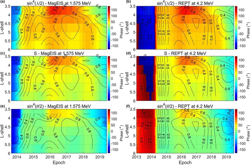
416 C. Katsavrias et al.: Semi-annual variation of outer belt electrons
are searching for common periodicities which are accompa- GOES/EPS. Note that the longer duration of available data
nied by high levels of coherence. The statistical significance from GOES/EPS allows us to compare the different SC
level of the WTC is estimated using Monte Carlo methods phases; thus, we plot the superposed epoch during three dif-
(see also Grinsted et al., 2004). ferent time periods: the whole dataset (solid blue line), the
ascending phase and maximum (solid red line) and the de-
scending phase (solid green line). As shown, the aforemen-
3 Results and discussion tioned asymmetry is exhibited at geostationary orbit as well.
Concerning the whole dataset (blue line), once again the first
3.1 Observations peak occurs during May, while the second one occurs si-
multaneously with the RM-predicted maximum, during early
Figure 2 presents the results of the superposed epoch anal- October. Similar behavior is exhibited concerning the sec-
ysis for the 0.346, 0.749, 1.575, 2.6, 3.4 and 4.2 MeV elec- ondary maxima. The flux during the descending phase (green
tron fluxes from MagEIS and REPT during the 2013–2019 line) exhibits the same behavior. On the other hand, the flux
time period, which corresponds to the late maximum and de- during the ascending and maximum phase (red line) exhibits
scending phase of SC24. The zero epoch time in each plot a completely different behavior. It increases up to a first
corresponds to the first day of the year (the extra day corre- peak which occurs between the equinoctial and RM predicted
sponding to leap years was not used as it is expected to have maxima and, then, forms a plateau with small variations up to
a negligible effect on the results). The data shown are daily July, when the predicted minimum of the RM hypothesis oc-
averages, further smoothed using a 28 d moving average win- curs. Then it decreases up to late September (predicted maxi-
dow in order to remove any effects of the solar rotation, while mum of the equinoctial mechanism) and forms a shorter lived
the vertical lines correspond to the equinoxes’ maxima and maximum during October. The evolution of the superposed
the summer solstice minimum derived by the three mecha- flux during the ascending phase and maximum of SC24 in-
nisms (Cliver et al., 2002). dicates that there is not only an asymmetry between the SC
It is evident that there are two distinct islets (peaks in rela- phases, but also that the SAV has almost disappeared.
tivistic electron flux) in all energy channels, centered roughly
on 4 < L < 5 (with the exception of 0.346 MeV, which spans 3.2 Semi-annual variation (SAV)
the 4 < L < 6 L shell range). In detail, the first peak oc-
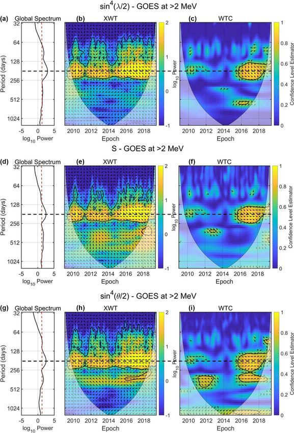
curs during May (approximately 1, 1.5 and 2 months after Figure 4 presents the time series, wavelet spectra (CWT)
the RM, equinoctial and axial maxima, respectively), while and global wavelet of the 0.346, 0.749, 1.575, 2.6, 3.4 and
the second one occurs almost simultaneously with the RM 4.2 MeV electron fluxes at 4.5 < L < 5 during the 2013–
maximum and lags ≈ 18 and ≈ 30 d behind the equinoctial 2019 time period. The black and red solid lines in the time
and axial maxima, respectively. Moreover, these peaks are series correspond to the daily values and to a 28 d moving
accompanied by secondary maxima (peaks at all energies average, respectively.
but with lower flux values than the aforementioned maxima), In order to reveal the SAV in the corresponding time se-
which occur almost simultaneously with the equinoctial and ries by eliminating the pronounced solar rotation, we have
axial maxima during March and September, respectively. applied a low-pass inverse Chebyshev filter (Williams and
This behavior has been observed before (see also Kanekal Taylors, 1988) with a cutoff period at 33 d; thus, the CWTs
et al., 2010, and Fig. 2 therein). Kanekal et al. (2010), using (and consequently the global spectra) are calculated using the
10 years of SAMPEX data (1993–2002), demonstrated that aforementioned filtered time series. The filtered time series
this asymmetry between the lags of the spring and autumn exhibit specific bands of periodic behavior with specific du-
equinox existed in both the descending phase of SC22 and ration, which is defined by the 95 % confidence level (black
the ascending phase of SC23, with the latter being even more contours in the CWT spectra). Moreover, the global spectrum
prominent than the former. They further suggested that this – which resembles a Fourier spectrogram – shows the fre-
asymmetry is either due to the limited dataset they used or quency range of each periodic band along with its maximum,
due to the different ways that high-speed streams and coro- while the dashed red line corresponds to the 95 % confidence
nal mass ejections energize relativistic electrons. We must level. We must note here that the 95 % confidence level in
note here that there can be no straightforward comparison be- the CWT and the global spectrum has a different meaning,
tween SAMPEX (low earth orbit and a broad range of equa- even though they are both sample-dependent. The former in-
torial pitch angles) and the dataset considered in this study dicates whether a specific variation is statistically significant
(near-equatorial elliptical orbit and near-equatorial pitch an- (or not) for a finite time period of the sample, while the latter
gles only). Nevertheless, our results indicate that this asym- indicates whether a specific variation is statistically signifi-
metry is equally prominent during the descending phase of cant for the entire sample.
SC24. As shown in the CWT and the global wavelet spectra of
Figure 3 shows the superposed epoch analysis using the corresponding time series, there is a pronounced SAV
integral flux measurements of > 2 MeV electrons from (maximum at ≈ 175 d) at all energy channels which spans
Ann. Geophys., 39, 413–425, 2021 https://doi.org/10.5194/angeo-39-413-2021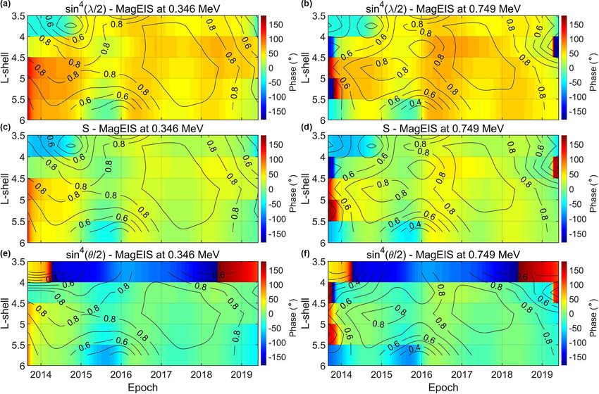
C. Katsavrias et al.: Semi-annual variation of outer belt electrons                                                                    417

Figure 2. Annual superposed epoch analysis showing 28 d moving average of electron fluxes (2013–2019) during the late maximum and
descending phase of SC24. Panels (a, c, e) correspond to MagEIS channels (top to bottom: 0.346, 0.749 and 1.575 MeV) and panels (b, d,
f) to REPT channels (top to bottom: 2.6, 3.4 and 4.2 MeV). Similar to Fig. 1, the vertical lines correspond to the equinoxes’ maxima and the
summer solstice minimum predicted by the three mechanisms (Cliver et al., 2002).

Figure 3. Annual superposed epoch analysis showing 28 d moving average electron fluxes at E > 2 MeV from GOES/EPS during three
time periods: the whole SC24 (solid blue line), the ascending phase and maximum (solid red line) and the descending phase (solid green
line). Similar to Fig. 1, the vertical lines correspond to the equinoxes’ maxima and the summer solstice minimum predicted by the three
mechanisms (Cliver et al., 2002).

https://doi.org/10.5194/angeo-39-413-2021                                                           Ann. Geophys., 39, 413–425, 2021
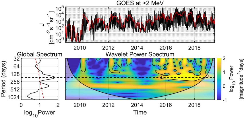
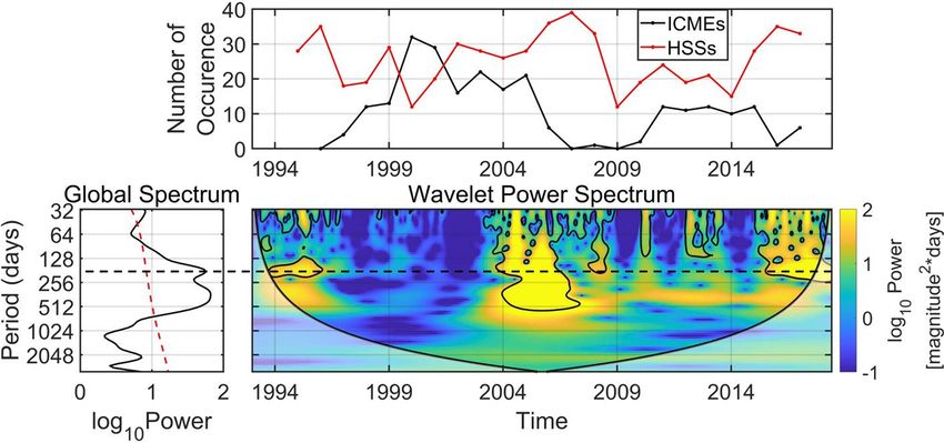
418                                                           C. Katsavrias et al.: Semi-annual variation of outer belt electrons

Figure 4. Time series, wavelet power (CWT) and global wavelet spectra of (a) 0.346, (b) 0.749, (c) 1.575, (d) 2.6, (e) 3.4 and (f) 4.2 MeV
electron fluxes at 4.5 < L < 5; the red lines are a 28 d moving average smoothing of the time series. The wavelet power display is color-
coded, with yellow corresponding to the maxima; the black line is the cone of influence of the spectra, where edge effects in the processing
become important, while the black contours correspond to the 95 % confidence level. The dashed red lines in the global spectra represent the
95 % confidence level of the global power. The horizontal dashed (black) lines highlight the SAV.

the time period 2015–2018. Furthermore, the SAV seems to                electrons. Grandin et al. (2019) studied the solar wind HSSs
be completely absent during the late maximum of the SC24                emanating from coronal holes during 1995–2017, encom-
(2013–2014) as well as 2019; nevertheless, most of the afore-           passing three descending phases (SC22, SC23 and SC24).
mentioned time period falls inside the cone of influence. Note             In order to investigate the aforementioned scenario, we
that the SAV is present in the descending phase of SC24 at              compared the CWT of > 2 MeV electron fluxes from
all energy channels (E > 100 keV) and at L > 3.5, while at              GOES/EPS with the number of occurrence of interplane-
L < 3.5 (not shown here) it is mostly below the 95 % confi-             tary coronal mass ejections (ICMEs) and HSSs during 1993–
dence level.                                                            2019 (taken from Figs. 3 and 5 in Grandin et al., 2019).
   Figure 5 shows the CWT of the > 2 MeV electron flux                  As shown in Fig. 6, the SAV occurs during all three de-
from GOES/EPS during the whole SC24 (2009–2019). As                     scending phases, roughly during 1994–1996, 2004–2007 and
shown, the SAV is exhibited at GEO, once again, with pro-               2015–2018. The common feature between the occurrences
nounced power (above the 95 % confidence level) during the              of the SAV is the simultaneous increase (decrease) of HSS
descending phase of SC24, while it is absent from any other             (ICMEs), with the exception of 2004 and 2005 where both
time period in the dataset. This behavior is in agreement with          are increased. These results indicate that the SAV in the rel-
the results shown in Fig. 3. As mentioned before, Kanekal               ativistic electrons at GEO is not only a manifestation of the
et al. (2010) argued that a possible explanation for the ob-            different reconnection rates produced by the equinoctial/RM
served asymmetry between ascending and descending SC                    mechanisms, but also a combination of the latter with the
phase is the different way that high-speed streams (hencefor-           simultaneous occurrence (absence) of HSSs (ICMEs). We
ward HSSs) and coronal mass ejections energize relativistic             must note here that during periods of high occurrence of both

Ann. Geophys., 39, 413–425, 2021                                                          https://doi.org/10.5194/angeo-39-413-2021
C. Katsavrias et al.: Semi-annual variation of outer belt electrons                                                           419

Figure 5. Same as Fig. 4 for the > 2 MeV electron fluxes from GOES/EPS during the whole SC24 from 2009 until 2019. The horizontal
dashed (black) line highlights the SAV.

ICMEs and HSSs, the effect of coherent magnetic structure           panels exhibits the maximum power during the descending
such as an ICME (or at least its magnetic cloud which can           phase of SC24. Moreover, it appears with reduced (but
cause long-lasting southward IMF and, thus, long-lasting re-        still significant) power during 2012–2013 and 2009–2010.
connection) is far more prominent than the modulation of            Note, that during 2014, where the SAV fades, we have the
reconnection produced by the variability of the controlling         maximum activity of SC24 in terms of the Solar Flare Index
angles of the equinoctial/RM mechanisms.                            provided by the National Oceanic and Atmospheric Admin-
                                                                    istration (NOAA; see also https://www.ngdc.noaa.gov/stp/
3.3   Common periodic behavior and phase relationship               space-weather/solar-data/solar-features/solar-flares/index/,
                                                                    last access: 7 May 2021).
                                                                       The phase relationship between the flux and the three func-
In order to investigate the effect of each mechanism (axial,
                                                                    tions is significant during the descending phase of SC24
equinoctial and RM) on the generation of the SAV in the rela-
                                                                    (2015–2018) only; a time period during which the maximum
tivistic electron fluxes, we use specific functions of the afore-
                                                                    power of the cross-spectrum occurs, as well. The important
mentioned angles instead of the angles themselves. For the
                                                                    difference in the cross-spectra between the flux and the three
ψ angle, which controls the equinoctial mechanism, we use
                                                                    functions lies in the phase relationship. As shown in both
the Svalgaard (1977) function: S = 1.157 · [1 + 3 · cos (90◦ −
                                                                    XWT and WTC, the θ function of the RM effect is the only
ψ)2 ]−2/3 . Moreover, similar to Akasofu (1981), we use the
                                                                    one in-phase with the electron flux at GEO during the whole
θ and λ angles, which control the RM and the axial mech-
                                                                    descending phase (arrows continuously pointing to the right).
anism, respectively, as sin(θ/2)4 and sin(λ/2)4. Figure 7
                                                                    On the other hand, the λ exhibits a ≈ 80–90◦ phase, which
shows the cross-wavelet transform (XWT) and wavelet co-
                                                                    corresponds to a ≈ 39–44 d time lag, while the S function ex-
herence (WTC) calculations used to study the interrelation of
                                                                    hibits a ≈ 30◦ phase, which corresponds to a ≈ 15 d time lag.
the > 2 MeV electron flux from GOES/EPS and the three pa-
                                                                    These time lags and the phase relationships are in agreement
rameters at geostationary orbit during the whole SC24. The
                                                                    with the results presented in Fig. 3 concerning the second
middle panels show the XWT spectrum of the two time se-
                                                                    maximum near the autumn equinox. They further indicate
ries under examination. The left-hand panels depict the time
                                                                    that the observed SAV at the > 2 MeV electron flux at GEO
average of the XWT spectrum, which once again resembles
                                                                    during the descending phase of SC24 is primarily driven by
a Fourier periodogram, and the right-hand panels the WTC.
                                                                    the RM mechanism.
The latter is the correlation coefficient of the time series
                                                                       Figure 8 shows the phase relationship between relativistic
wavelet transform phase. Arrows indicate the phase relation-
                                                                    electron fluxes (0.346 and 0.749 MeV) from MagEIS and the
ship between the two time series in time–frequency space:
                                                                    three angle functions as inferred from the XWT spectrum as
those pointing to the right correspond to in-phase behavior
                                                                    a function of L shell and time. The phase is color-coded, with
and those to the left anti-phase. The downwards-pointing ar-
                                                                    green corresponding to 0◦ . The black contours correspond to
rows indicate 90◦ lead of the first dataset, meaning that the
                                                                    the coherence level estimator as inferred from WTC. Note
first dataset occurs earlier in time.
                                                                    that we only show data at L > 3.5 since the SAV in both the
   As shown, the SAV is shared between the > 2 MeV elec-
                                                                    CWT and the XWT is below the 95 % confidence level at
tron flux and all three parameters with a maximum power at
                                                                    L < 3.5.
≈ 175 d (left-hand panels of Fig. 7). In detail, the SAV in all

https://doi.org/10.5194/angeo-39-413-2021                                                    Ann. Geophys., 39, 413–425, 2021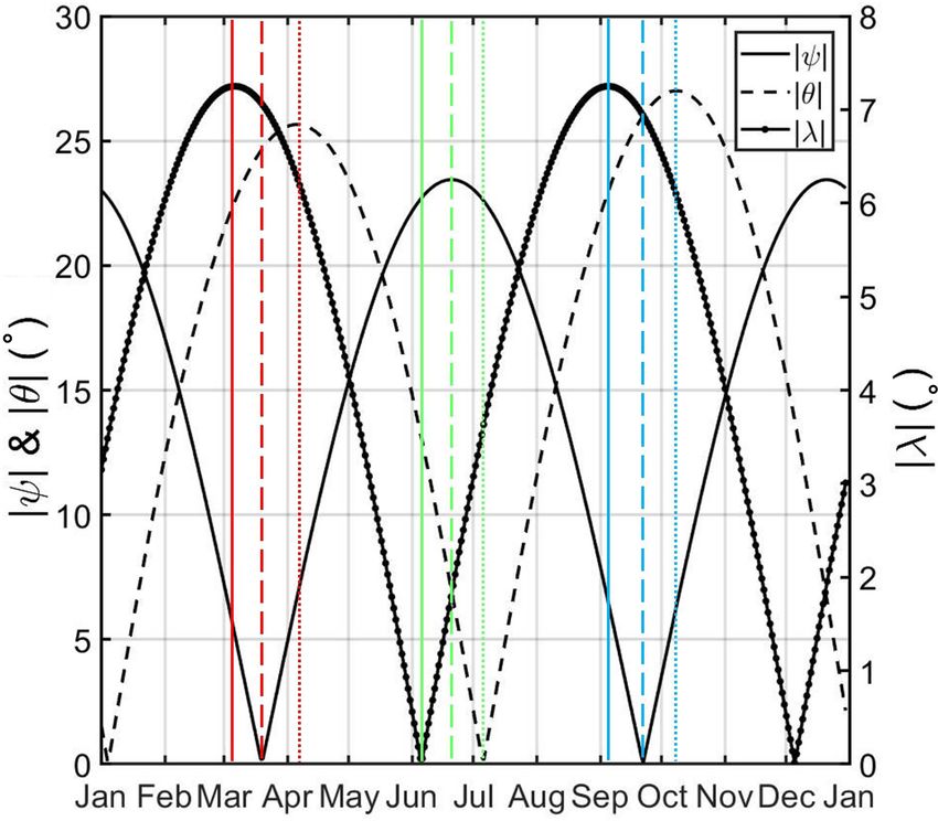
420                                                       C. Katsavrias et al.: Semi-annual variation of outer belt electrons

Figure 6. Comparison of the occurrence of the SAV in the > 2 MeV electron flux from GOES/EPS and the number of occurrence of ICMEs
and HSSs during the 1993–2019 time period. The horizontal dashed (black) line highlights the SAV.

   As shown, the results in the outer radiation belt are in        multiple SCs and with various in situ data renders the con-
agreement with the results at GEO (see also Fig. 7). In both       clusions significantly important.
energy channels, the SAV exhibits an in-phase relationship            Moreover, as shown in the previous sections, the presence
with the θ function, which controls the RM effect. We em-          of the SAV in the relativistic electrons of the outer belt co-
phasize the fact that the deviations in-phase are within the       incides with enhanced HSS occurrence during the descend-
0–10◦ range, corresponding to a maximum time lag of 5 d.           ing phase of the SC. This was also indicated by Baker et
This behavior is consistent at the 4 < L < 5.5 range during        al. (1999), who proposed the following scenario: substorm
the late 2014–2018 time period, with coherence levels > 0.6.       injections are enhanced due to the effective southward IMF
At L > 5.5 the in-phase relationship between the flux and the      component, which, in turn, is favored by the RM effect (and
θ function is limited in the 2016–2018 time period. On the         other factors). Then the injected source–seed populations of
other hand, the phase relationship between the flux and the        low-energy electrons into the inner magnetosphere are accel-
S (λ) function is mostly ≈ 30 (≈ 90)◦ , which, as mentioned        erated by ultralow-frequency (ULF) waves produced by the
before, corresponds to a ≈ 15 (45) d time lag. As we move          Kelvin–Helmholtz instability, which is favored by the HSSs.
to higher electron energy (Fig. 9), there are small deviations     McPherron et al. (2009) provided further evidence on the va-
from the aforementioned pattern. At 1.575 and 4.2 MeV, the         lidity of the aforementioned scenario, highlighting the im-
flux is in-phase with the θ function, with coherence levels        portance of the azimuthal electric field (Ey). Similar results
exceeding the 0.6 level mostly during the 2015–2018 time           were reported by Smirnov et al. (2019) and Katsavrias et al.
period and at L > 4.5. As in the lower energy channels,            (2021) using Cluster/RAPID and GOES/MAGED data, re-
the phase relationship between 1.575 and 4.2 MeV electron          spectively. On the other hand, Kanekal et al. (2010) showed
fluxes and the S (λ) function is mostly ≈ 30 (≈ 90)◦ .             that radial diffusion could not explain the simultaneous and
                                                                   rapid flux peaks over a broad range of L shells and proposed
3.4   Discussion                                                   that, even though the HSSs were responsible for the elevated
                                                                   fluxes during the equinoxes of the descending phase, in situ
These results verify that the SAV in the relativistic electron     acceleration rather than radial transport process may domi-
fluxes of the outer radiation belt is primarily driven by the      nate electron energization.
RM effect, which in turn is controlled by the θ angle and,            Regardless of the acceleration process, all aforementioned
moreover, is present during the descending phase of SC24           authors agree on the dependence of SAV (and consequently
(2015–2019). Nevertheless, we cannot exclude some con-             of the electron flux increase around the equinoxes) on the
tribution from the equinoctial mechanism as well, since the        combination of HSSs and the RM effect. Nevertheless, we
variation of the phase between electron fluxes and the S func-     must note that recent studies have shown that HSSs are
tion can reach ≈ 15◦ , which corresponds to a ≈ 7.5 d time         equally (or more) effective in enhancing ultrarelativistic elec-
lag. The derived results are in agreement with Kanekal et          trons than a major geomagnetic storm produced by an ICME
al. (2010), who argued that the times of peak fluxes of rel-       (Horne et al., 2018; Katsavrias et al., 2019b).
ativistic electrons lag behind the nominal equinoxes signifi-         Finally, there is still an open question left concerning
cantly, and, therefore, the equinoctial mechanism cannot ac-       the observed asymmetry between the spring and autumn
count for the observed SAV as previously suggested by Li et
al. (2001). The fact that these results are consistent through

Ann. Geophys., 39, 413–425, 2021                                                   https://doi.org/10.5194/angeo-39-413-2021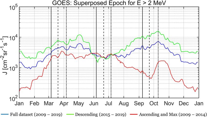
C. Katsavrias et al.: Semi-annual variation of outer belt electrons                                                                        421

Figure 7. Global wavelet (a, d, g), cross-wavelet transformation (XWT; b, e, h) and wavelet coherence (WTC; c, f, i) between the > 2 MeV
electron flux from GOES/EPS and the λ function (a, b, c), the S function (d, e, f) and the θ function (g, h, i); the dashed red line corresponds
to the 95 % confidence level of the global wavelet. The thick black contours mark the 95 % confidence level, and the thin line indicates the
cone of influence (COI). The color bar of the XWT indicates the log10(power); the color bar of the WTC corresponds to the confidence
level of the phase obtained by the Monte Carlo test, and the arrows correspond to a confidence level > 0.6. The arrows point to the phase
relationship of the two data series in time–frequency space: (1) arrows pointing to the right indicate in-phase behavior; (2) arrows pointing
to the left indicate anti-phase behavior; (3) arrows pointing downward indicate that the first dataset is leading the second (meaning that the
first dataset occurs earlier in time) by 90◦ . The horizontal dashed (black) lines highlight the SAV.

https://doi.org/10.5194/angeo-39-413-2021                                                              Ann. Geophys., 39, 413–425, 2021
422                                                             C. Katsavrias et al.: Semi-annual variation of outer belt electrons

Figure 8. Phase relationship between electron fluxes and the three angle functions as inferred from the XWT spectrum as a function of L
shell and time. Panels (a, c, e) correspond to 0.346 and panels (b, d, f) to 0.749 MeV electrons from MagEIS. The phase relationship between
the flux and λ (a, b), ψ (c, d) and θ (e, f) functions, which control the axial, equinoctial and RM mechanism, respectively. The black contours
correspond to the coherence level estimator as inferred from WTC.

Figure 9. Same as Fig. 8 for the 1.575 MeV electron flux from MagEIS (a, c, e) and 4.2 MeV electron flux from REPT (b, d, f).

equinox, which cannot be explained by the phase variation                 ments on board RBSP in order to investigate not only the oc-
inferred from this study.                                                 currences, but also the drivers of the SAV of the relativistic
                                                                          electron fluxes in the outer radiation belt.
                                                                             Our results indicate that the SAV in the relativistic elec-
4     Conclusions                                                         tron fluxes at both GEO and the outer radiation belt (L >
                                                                          4) is exhibited during the descending phase SC24, roughly
In this work we have exploited a broad energy range dataset               spanning the 2015–2018 time period. In order to investigate
(≈ 0.3–4.2 MeV) provided by the MagEIS and REPT instru-

Ann. Geophys., 39, 413–425, 2021                                                            https://doi.org/10.5194/angeo-39-413-2021
C. Katsavrias et al.: Semi-annual variation of outer belt electrons 423
the consistency of this result during different SCs, we used static models, while it should be noted that these relatively
the > 2 MeV integral electron fluxes derived from the Ener- short-scale dynamics are of particular interest for short-lived
getic Particle Sensor (EPS) on board the geostationary GOES missions (e.g., electric orbit-raising trajectories or short-lived
satellites, covering almost three SCs from January 1993 to nanosats).
July 2019. The wavelet spectrum showed that the SAV oc-
curred during all three descending phases and, moreover, co-
existed with periods of an increased (decreased) number of Code availability. The software code for MATLAB can be
HSS (ICME) occurrence, indicating that the SAV is a result found at https://noc.ac.uk/business/marine-data-products/
of the modulation of reconnection produced by the variabil- cross-wavelet-wavelet-coherence-toolbox-matlab (Grinsted et
ity of the controlling angles of the RM (and/or equinoctial) al., 2004).
mechanism during periods of enhanced solar wind speed.
Unfortunately, this conclusion can be verified only at GEO
Data availability. The datasets for the RBSP and GOES data are
since RBSP data cover less than a full SC.
available at https://www.rbsp-ect.lanl.gov/science/DataDirectories.
Furthermore, we applied the cross-wavelet and wavelet co-
php (Radiation Belt Storm Probes ECT, 2021) and https://satdat.
herence techniques in order to investigate the phase relation- ngdc.noaa.gov/sem/goes/data/ (NOAA, 2021) respectively.
ship between the relativistic electron fluxes and the control-
ling angles of the axial, equinoctial and RM mechanisms.
Our results indicate that the SAV in the relativistic elec- Author contributions. CK drafted and wrote the paper, with partic-
trons of the outer radiation belt is primarily driven by the ipation of all coauthors. CP and SAG contributed to software devel-
RM effect, without excluding a small contribution from the opment. IS, IAD and PJ were consulted regarding the data analysis
equinoctial mechanism. and interpretation of the results.
The aforementioned results can be used to refine ongoing
developments or further contribute to radiation belt modeling
endeavors. Several specification models of the outer radiation Competing interests. The authors declare that they have no conflict
belt are used by the engineering community to design both of interest.
the orbital characteristics of future missions and the shield-
ing of sensitive instruments on board. Unfortunately, most of
these are either completely static or include time variations Acknowledgements. This work has received funding from the Eu-
in an overly simplistic manner. As an example, the standard ropean Union’s Horizon 2020 Research and Innovation programme
“SafeSpace” (grant agreement no. 281 870437) and from the Eu-
AE-8 model only comes in two versions for active (AE-8
ropean Space Agency under the “European Contribution to Inter-
MAX) and quiet (AE-8 MIN) solar conditions (Vette, 1991).
national Radiation Environment Near Earth (IRENE) Modelling
The successor to AE-8, AE-9 (Ginet et al., 2013), is mostly System” activity (ESA contract no. 4000127282/19/NL/IB/gg).
static, only exhibiting time dependence for specific periodic- The MATLAB package of the National Oceanography Centre,
ities (including a 6-month one) in a random fashion, using Liverpool, UK, was used in the calculation of the CWT, XWT
a Monte Carlo approach. On the other hand, the ONERA and WTC. The authors acknowledge the RBSP/MagEIS and
models MEO (Lazaro et al., 2009) and IGE-2006 (Sicard- RBSP/REPT teams for the use of the corresponding datasets
Piet et al., 2008) do exhibit a proper solar cycle dependence, which can be found online at https://www.rbsp-ect.lanl.gov/science/
but these models are built using yearly averages and thus DataDirectories.php (last access: 7 May 2021) and the developers of
cannot account for shorter periodicities. A new category of the International Radiation Belt Environment Modeling (IRBEM)
models that has emerged in recent years is machine learning library that was used to calculate the theoretical angles of the axial,
equinoctial and Russell–McPherron mechanisms. The GOES/EPS
models, such as the very recent MERLIN model (Smirnov
data are retrieved from https://satdat.ngdc.noaa.gov/sem/goes/data/
et al., 2020). These are typically built on many years of data (last access: 7 May 2021).
and thus probably include the effects of all such variabili-
ties but in a way that is difficult to disentangle from all the
other effects and variations. Even in these cases though, our Financial support. This research has been supported by the Euro-
study can help in the choice of input parameters that when pean Union’s Horizon 2020 Research and Innovation programme
included in a machine learning model will assist it in prop- (SafeSpace (grant no. 281 870437)) and from the European Space
erly representing this type of phenomenon. Finally, physics- Agency under the “European Contribution to International Radia-
based models are typically run using the value of a specific tion Environment Near Earth (IRENE) Modelling System” activity
geomagnetic activity index as input or a larger set of obser- (ESA contract no. 4000127282/19/NL/IB/gg).
vations of the interplanetary conditions, and thus they require
accurate predictions of these parameters long into the future.
Conversely to all these, incorporating the semi-annual vari- Review statement. This paper was edited by Elias Roussos and re-
ability can be easily performed for any point in time, and this viewed by two anonymous referees.
helps produce more realistic outputs from even completely
https://doi.org/10.5194/angeo-39-413-2021 Ann. Geophys., 39, 413–425, 2021424 C. Katsavrias et al.: Semi-annual variation of outer belt electrons
References Daglis, I. A., Katsavrias, C., and Georgiou, M.: From so-
lar sneezing to killer electrons: outer radiation belt re-
sponse to solar eruptions, Philos. T. Roy. Soc. A, 377,
Akasofu, S. I.: Energy coupling between the so- https://doi.org/10.1098/rsta.2018.0097, 2019.
lar wind and the magnetosphere, 28, 121–190, Emery, B. A., Richardson, I. G., Evans, D. S., Rich, F. J, and Wil-
https://doi.org/10.1007/BF00218810, 1981. son, G. R.: Solar Rotational Periodicities and the Semiannual
Baker, D. N., Kanekal, S. G., Pulkkinen, T. I., and Blake, J. B.: Variation in the Solar Wind, Radiation Belt, and Aurora, Sol.
Equinoctial and solstitial averages of magnetospheric relativistic Phys., 274, 399–425, https://doi.org/10.1007/s11207-011-9758-
electrons: A strong semiannual modulation, Geophys., Res. Lett., x, 2011.
26, 3193–3196, https://doi.org/10.1029/1999GL003638, 1999. Ginet, G. P., O’Brien, T. P., Huston, S. L., Johnston, W. R., Guild,
Baker, D. N., Kanekal, S. G., Hoxie, V. C., Batiste, S., Bolton, M., T. B., Friedel, R., Lindstrom, C. D., Whelan, P., Quinn, R. A.,
Li, X., Elkington, S. R., Monk, S., Reukauf, R., Steg, S., Westfall, Madden, D., Morley, S., and Su, Y.-J.: AE9, AP9 and SPM:
J., Belting, C., Bolton, B., Braun, D., Cervelli, B., Hubbell, K., New Models for Specifying the Trapped Energetic Particle and
Kien, M., Knappmiller, S., Wade, S., Lamprecht,B., Stevens, K., Space Plasma Environment, Space Sci. Rev., 179, 579–615,
Wallace, J., Yehle, A., Spence, H. E., and Friedel, R.: The Rela- https://doi.org/10.1007/s11214-013-9964-y, 2013.
tivistic Electron–Proton Telescope (REPT) instrument on board Grandin, M., Aikio, A. T., and Kozlovsky, A.: Properties and geo-
the Radiation Belt Storm Probes (RBSP) spacecraft: Characteri- effectiveness of solar wind high-speed streams and stream inter-
zation of Earth’s radiation belt high–energy particle populations, action regions during solar cycles 23 and 24, J. Geophys. Res.-
Space Sci. Rev., 65, 1385–1398, https://doi.org/10.1007/s11214- Space, 124, 3871–3892, https://doi.org/10.1029/2018JA026396,
012-9950-9, 2012. 2019.
Blake, J. B., Carranza, P. A., Claudepierre, S. G., Clemmons, J. Grinsted, A., Moore, J. C., and Jevrejeva, S.: Application
H., Crain, W. R, Dotan, Y., Fennell, J. F., Fuentes, F. H., Gal- of the cross wavelet transform and wavelet coherence to
van, R. M., George, J. S., Henderson, M. G., Lalic, M., Lin, geophysical time series, Nonlin. Processes Geophys., 11,
A. Y., Looper, M. D., Mabry, D. J., Mazur, J. E., McCarthy, 561–566, https://doi.org/10.5194/npg-11-561-2004, 2004 (data
B., Nguyen, C. Q., O’Brien, T. P., Perez, M. A., Redding, M. available at: https://noc.ac.uk/business/marine-data-products/
T., Roeder, J. L., Salvaggio, D. J., Sorensen, G. A., Spence, H. cross-wavelet-wavelet-coherence-toolbox-matlab, last access:
E., Yi, S., and Zakrzewski, M. P.: The Magnetic Electron Ion 7 May 2021).
Spectrometer (MagEIS) instruments aboard the Radiation Belt Horne, R. B., Phillips, M. W., Glauert, S. A., Meredith, N.
Storm Probes (RBSP) spacecraft, Space Sci. Rev., 179, 383–421, P., Hands, A. D. P., Ryden, K. A., and Li, W.: Realistic
https://doi.org/10.1007/s11214-013-9991-8, 2013. Worst Case for a Severe Space Weather Event Driven by
Bourdarie, S. and O’Brien, T. P.: International Radiation Belt En- a Fast Solar Wind Stream, Space Weather, 16, 1202–1215,
vironment Modelling Library, Space Res. Today, 174, 27–28, https://doi.org/10.1029/2018SW001948, 2018.
https://doi.org/10.1016/j.srt.2009.03.006, 2009. Kanekal, S. G., Baker, D. N., and McPherron, R. L.: On the seasonal
Boyd, A. J., Reeves, G. D., Spence, H. E., Funsten, H. O., dependence of relativistic electron fluxes, Ann. Geophys., 28,
Larsen, B. A., Skoug, R. M., Blake, J. B., Fennell, J. F., 1101–1106, https://doi.org/10.5194/angeo-28-1101-2010, 2010.
Claudepierre, S. G., Baker, D. N., Kanekal, S. G., and Katsavrias, C., Daglis, I. A., Li, W., Dimitrakoudis, S., Geor-
Jaynes, A. N.: RBSP-ECT combined spin-averaged electron giou, M., Turner, D. L., and Papadimitriou, C.: Com-
flux data product, J. Geophys. Res.-Space, 124, 9124–9136, bined effects of concurrent Pc5 and chorus waves on rel-
https://doi.org/10.1029/2019JA026733, 2019. ativistic electron dynamics, Ann. Geophys., 33, 1173–1181,
Chapman, S. and Bartels, J.: Geomagnetism, vol. 2, Oxford Univer- https://doi.org/10.5194/angeo-33-1173-2015, 2015.
sity Press, London, UK, p. 601, 1940. Katsavrias, C., Hillaris, A., and Preka-Papadema, P.: A wavelet
Claudepierre, S. G., O’Brien, T. P., Blake, J. B., Fennell, J. F., based approach to Solar–Terrestrial Coupling, Adv. Space Res.,
Roeder, J. L., Clemmons, J. H., Looper, M. D., Mazur, J. E., 57, 2234–2244, https://doi.org/10.1016/j.asr.2016.03.001, 2016.
Mulligan, T. M., Spence, H. E., Reeves, G. D., Friedel, R. Katsavrias, C., Daglis, I. A., and Li, W.: On the statistics of ac-
H. W., Henderson, M. G., and Larsen, B. A.: A background celeration and loss of relativistic electrons in the outer radiation
correction algorithm for Van Allen Probes MagEIS electron belt: A superposed epoch analysis, J. Geophys. Res.-Space, 124,
flux measurements, J. Geophys. Res.-Space, 120, 5703–5727, 2755–2768, https://doi.org/10.1029/2019JA026569, 2019a.
https://doi.org/10.1002/2015JA021171, 2015. Katsavrias, Ch., Sandberg, I., Li, W., Podladchikova, O., Daglis,
Cliver, E. W., Kamide, Y., and Ling, A. G.: Mountains vs. valleys: I. A., Papadimitriou, C., Tsironis, C., Aminalragia-Giamini, S.:
the semiannual variation of geomagnetic activity, J. Geophys. Highly relativistic electron flux enhancement during the weak
Res., 105, 2413–2424, https://doi.org/10.1029/1999JA900439, geomagnetic storm of April–May 2017, J. Geophys. Res.-Space,
2000. 124, 4402–4413, https://doi.org/10.1029/2019JA026743, 2019b.
Cliver, E. W., Kamide, Y., and Ling, A.: The semiannual Katsavrias, C., Aminalragia-Giamini, S., Papadimitriou, C. Sand-
variation of geomagnetic activity: phases and profiles for berg, I., Jiggens, P., Daglis, I. A., and Evans, H.: On the In-
130 years of aa data, J. Atmos. Solar Terr. Phys., 64, 47–53, terplanetary Parameter Schemes which Drive the Variability of
https://doi.org/10.1016/S1364-6826(01)00093-1, 2002. the Source/Seed Electron Population at GEO, J. Geophys. Res.-
Cortie, A. L.: Sunspots and terrestrial magnetic phenomena, Space, accepted, 2021.
1898–1911: the cause of the annual variation in mag-
netic disturbances, Mon. Not. R. Astron. Soc., 73, 52–60,
https://doi.org/10.1093/mnras/73.1.52, 1912.
Ann. Geophys., 39, 413–425, 2021 https://doi.org/10.5194/angeo-39-413-2021C. Katsavrias et al.: Semi-annual variation of outer belt electrons 425 Lazaro, D., Bourdarie, S., Ryden, K., Hands, A., Underwood, C., Smirnov, A. G., Kronberg, E. A., Latallerie, F., Daly, P. W., and Ecoffet, R.: MEO Final Report, ESA/ESTEC CONTRACT Aseev, N., Shprits, Y. Y., Kellerman, A., Kasahara, S., Turner, NO. 21403/08/NL/JD, 2009. D., and Taylor, M. G. G. T. : Electron intensity measure- Li, X., Baker, D. N., Kanekal, S. G., Looper, M., and Temerin, ments by the Cluster/RAPID/IES instrument in Earth’s ra- M.: Long term measurements of radiation belts by SAM- diation belts and ring current, Space Weather, 17, 553–566, PEX and their variations, Geophys. Res. Lett., 28, 3827–3830, https://doi.org/10.1029/2018SW001989, 2019. https://doi.org/10.1029/2001GL013586, 2001. Smirnov, A. G., Berrendorf, M., Shprits, Y. Y., Kronberg, E. A., Maraun, D. and Kurths, J.: Cross wavelet analysis: significance Allison, H. J., Aseev, N. A., Zhelavskaya, I. S., Morley, S. K., testing and pitfalls, Nonlin. Processes Geophys., 11, 505–514, Reeves, G. D., Carver, M. R., and Effenberger, F.: Medium en- https://doi.org/10.5194/npg-11-505-2004, 2004. ergy electron flux in earth’s outer radiation belt(MERLIN): A McPherron, R. L., Baker, D. N., and Crooker, N. U.: Role of machine learning model, Space Weather, 18, e2020SW002532, the Russell–McPherron effect in the acceleration of relativis- https://doi.org/10.1029/2020SW002532, 2020. tic electrons, J. Atmos. Solar Terr. Phys., 71, 1032–1044, Svalgaard, L.: Geomagnetic activity: Dependence on solar wind pa- https://doi.org/10.1016/j.jastp.2008.11.002, 2009. rameters, in: Coronal Holes and High Speed Wind Streams, Col- Morlet, J.: Sampling Theory and Wave Propagation, in: Issues in orado Association University Press, Boulder, Colorado, USA, Acoustic Signal – Image Processing and Recognition, edited 371, 1977. by: Chen, C. H., NATO ASI Series (Series F: Computer Torrence, C. and Compo, G. P.: A Practical and System Sciences), vol. 1., Springer, Berlin, Heidelberg, Guide to Wavelet Analysis, B. Am. Meteo- https://doi.org/10.1007/978-3-642-82002-1_12, 1983. rol. Soc., 79, 61–78, https://doi.org/10.1175/1520- National Oceanic and Atmospheric Administration (NOAA): 0477(1998)0792.0.CO;2, 1998. GOES/EPS, available at: https://satdat.ngdc.noaa.gov/sem/goes/ Tsyganenko, N. A. and Sitnov, M. I.: Modeling the dy- data/, last access: 7 May 2021, 2021. namics of the inner magnetosphere during strong geo- Onsager, T. G., Grubb, R., Kunches, J., Matheson, L., Speich, D., magnetic storms, J. Geophys. Res.-Space, 110, A03208, Zwickl, R., and Sauer, H.: Operational uses of the GOES en- https://doi.org/10.1029/2004JA010798, 2005. ergetic particle detectors, Proc. SPIE Int. Soc. Opt. Eng., 2812, Turner, D. L., O’Brien, T. P., Fennell, J. F., Claudepierre, 281, 1996. S. G., Blake, J. B., Kilpua, E. K. J., and Hietala, H.: Poblet, F. L., Azpilicueta, F., and Lam, H.-L.: Semiannual variation The effects of geomagnetic storms on electrons in Earth’s of Pc5 ultra-low frequency (ULF) waves and relativistic electrons radiation belts, Geophys. Res. Lett., 42, 9176–9184, over two solar cycles of observations: comparison with predic- https://doi.org/10.1002/2015GL064747, 2015. tions of the classical hypotheses, Ann. Geophys., 38, 953–968, Usanova, M. E., Drozdov, A., Orlova, K., Mann, I. R., Shprits, https://doi.org/10.5194/angeo-38-953-2020, 2020. Y., Robertson, M. T., Turner, D. L., Milling, D. K., Kale, A., Radiation Belt Storm Probes ECT: RBSP-ECT Science Data Baker, D. N., Thaller, S. A., Reeves, G. D., Spence, H. E., Klet- Products, available at: https://www.rbsp-ect.lanl.gov/science/ zing, C., and Wygant, J.: Effect of EMIC waves on relativistic DataDirectories.php, last access: 7 May 2021. and ultrarelativistic electron populations: Groundbased and Van Reeves, G. D., McAdams, K. L., Friedel, R. H. W., and Allen Probes observations, Geophys. Res. Lett., 41, 1375–1381, O’Brien, T. P.: Acceleration and loss of relativistic electrons https://doi.org/10.1002/2013GL059024, 2014. during geomagnetic storms, Geophys. Res. Lett., 30, 1529, Vette, J. I.: The AE-8 Trapped Electron Model Environment, https://doi.org/10.1029/2002GL016513, 2003. NSSDC report 91-24, NSSDC, 1991. Reeves, G. D. and Daglis, I. A.: Geospace Magnetic Storms and the Williams, A. B. and Taylors, F. J.: Electronic Filter Design Hand- Van Allen Radiation Belts, in: Waves, Particles and Storms in book, McGraw-Hill, New York, USA, ISBN 0-07-070434-1, Geospace, edited by: Balasis, G., Daglis, I. A., and Mann, I. R., 1988. Oxford University Press, Oxford, UK, 2016. Russell, C. T. and McPherron, R. L.: Semiannual variation of geomagnetic activity, J. Geophys. Res., 78, 92–108, https://doi.org/10.1029/JA078i001p00092, 1973. Sicard-Piet, A., Bourdarie, S., Boscher, D., Friedel, R. H. W., Thomsen, M., Goka, T., Matsumoto, H., and Koshiishi, H.: A new International Geostationary Electron model: IGE- 2006, from 1 keV to 5.2 MeV, Space Weather, 6, S07003, https://doi.org/10.1029/2007SW000368, 2008. https://doi.org/10.5194/angeo-39-413-2021 Ann. Geophys., 39, 413–425, 2021
You can also read