Continuous national gross domestic product (GDP) time series for 195 countries: past observations (1850-2005) harmonized with future projections ...
←
→
Page content transcription
If your browser does not render page correctly, please read the page content below
Earth Syst. Sci. Data, 10, 847–856, 2018
https://doi.org/10.5194/essd-10-847-2018
© Author(s) 2018. This work is distributed under
the Creative Commons Attribution 4.0 License.

        Continuous national gross domestic product (GDP) time
        series for 195 countries: past observations (1850–2005)
         harmonized with future projections according to the
             Shared Socio-economic Pathways (2006–2100)
                                                        Tobias Geiger
              Potsdam Institute for Climate Impact Research, Telegraphenberg A 56, 14473 Potsdam, Germany
                                 Correspondence: Tobias Geiger (geiger@pik-potsdam.de)

                                    Received: 21 July 2017 – Discussion started: 24 August 2017
                           Revised: 26 March 2018 – Accepted: 27 March 2018 – Published: 27 April 2018

       Abstract. Gross domestic product (GDP) represents a widely used metric to compare economic development
       across time and space. GDP estimates have been routinely assembled only since the beginning of the second
       half of the 20th century, making comparisons with prior periods cumbersome or even impossible. In recent years
       various efforts have been put forward to re-estimate national GDP for specific years in the past centuries and
       even millennia, providing new insights into past economic development on a snapshot basis. In order to make
       this wealth of data utilizable across research disciplines, we here present a first continuous and consistent data
       set of GDP time series for 195 countries from 1850 to 2009, based mainly on data from the Maddison Project
       and other population and GDP sources. The GDP data are consistent with Penn World Tables v8.1 and future
       GDP projections from the Shared Socio-economic Pathways (SSPs), and are freely available at http://doi.org/10.
       5880/pik.2018.010 (Geiger and Frieler, 2018). To ease usability, we additionally provide GDP per capita data
       and further supplementary and data description files in the online archive. We utilize various methods to handle
       missing data and discuss the advantages and limitations of our methodology. Despite known shortcomings this
       data set provides valuable input, e.g., for climate impact research, in order to consistently analyze economic
       impacts from pre-industrial times to the future.

1   Introduction                                                   of economic development within or across nations. Many
                                                                   other development proxies, e.g., the level of education, life
The concept of measuring and comparing economic activity           expectancy, the population’s health status, and many others,
within and across countries using the gross domestic prod-         have been shown to correlate well with a nation’s GDP; see,
uct (GDP) is rather new in historic terms. Starting with some      e.g., Gennaioli and La Porta (2013). Similarly, a reduction in
first attempts to quantify economic activity in the late 19th      vulnerability (or an increase in resilience) to natural disasters
century for certain countries, comprehensive regular assess-       has also been shown to correlate well with a nation’s GDP
ments of GDP were only established in the second half of           (Kousky, 2013), resulting in less mortality and in fewer dam-
the 20th century. Since then GDP has become the standard           ages relative to GDP. Most research in this field focuses only
indicator to assess nations’ development, despite initial and      on the last decades where sufficient coverage of economic ac-
more recent criticism concerning the incomplete representa-        tivity exists for most countries of the world. However, many
tion of a nation’s state via GDP and the potential problematic     fields of research could benefit from a more comprehensive
comparison across countries (Speich Chasse, 2013).                 economic data set that covers a larger time horizon and a
   Nonetheless and because of a lack of alternatives GDP           larger number of nations to gain a better understanding of
has proven to be a useful measure to track the evolution           the drivers of long-term economic development.

Published by Copernicus Publications.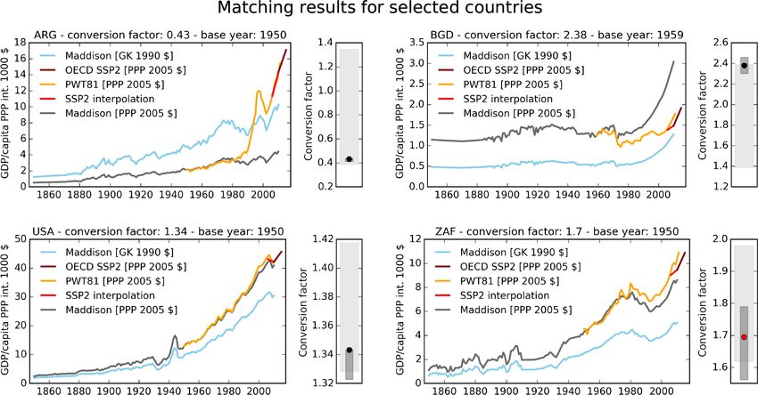
848                                    T. Geiger: Continuous national gross domestic product time series for 195 countries

   Various global institutions (e.g., Worldbank, Organisation    Table 1. Overview of data sources used to create the final data prod-
for Economic Co-operation and Development, OECD; In-             uct ranked according to their priority. Please refer to Sects. 2.1 and
ternational Monetary Fund, IMF) and research groups (e.g.,       2.2 for details on the data sources.
Penn World Table) have therefore assembled global GDP
                                                                       Data           Historical                    Future
data sets, most of which provide a comprehensive view
                                                                       priority      observations                 projections
across space but lack data prior to the 1960s. In addition,
there have been attempts to provide GDP or income (i.e.,                          Income   Population       Income     Population
GDP per capita) estimates reaching further back in time                1          PWT8.1   PWT8.1                OECD SSP2
based on proxies for specific periods; see, e.g., Baier et             2          MPD      HYDE                   –              –
al. (2002), Mitchel (2003), Maddison (2007), and Bolt and              3          PWT9.0   PWT9.0                 –              –
van Zanden (2014). However, these estimates only provide               4          WDI      WDI                    –              –
snapshots of economic activities for specific periods without
continuous global coverage across time.
   Here, we contribute to increasing the usability of histori-   2.1       Gross domestic product (GDP)
cal economic time series by creating a continuous and com-
                                                                 2.1.1      Penn World Tables (PWTs)
plete income and GDP time series from 1850 to the present.
We do so by combination of various data sources and meth-        The PWTs comprise national accounts data maintained by
ods to interpolate and extrapolate missing data points in        scholars at the University of California and the University
a pragmatic but most sensible way. The Maddison Project          of Groningen to measure real GDP across countries and
Database (MPD) thereby constitutes the foundation of the         over time. The database is successively updated and ex-
period mostly before 1960, while the Penn World Table (ver-      tended, with the latest release being PWT 9.0 (Feenstra et
sion 8.1) sets the basis for the more recent past. Our final     al., 2015), and provides the most extensive coverage for GDP
GDP time series covers 195 countries (in their present con-      reported in purchasing power parity (PPP) across time. We
stitution) from 1850 to 2009 and is consistent with GDP pro-     here mostly rely on the PWT release 8.1 from 2015 for
jections from the Shared Socio-economic Pathways (SSPs)          two reasons: first, PWT8.1 data are reported in 2005 PPP
that extend the historical time series from 2010 to 2100.        USD and are thus consistent with SSP projections. Second,
   The long record and complete coverage enhance the data        PWT8.1 is in close agreement with the SSP initial data in
set’s usability. It has already been assigned as input data      2010, thus reducing matching artefacts to a minimum. More-
for the current climate change impact model runs within the      over, PWT8.1 replaces the strongly criticized original PPPs
global Inter-sectoral Impact Model Intercomparison Project       for 2005; see, e.g., Deaton and Heston (2010), with a modi-
(ISIMIP2b) (Frieler et al., 2017), and has been used in a        fied version; see Inklaar and Rao (2017) for details. Missing
downscaling approach to provide spatially explicit economic      countries in PWT8.1 are taken from PWT9.0 after rescaling
information on the grid level (Geiger et al., 2017; Murakami     from 2011 to 2005 PPP USD; see the discussion below. PWT
and Yamagata, 2017) that can, e.g., be used to quantify          also provides national population estimates that we apply to
economic values exposed to climate extremes (Geiger et           generate income estimates based on national GDP.
al., 2018). Despite various known shortcomings that are dis-
cussed in detail below, this new data set has broadened and
                                                                 2.1.2      World Development Indicators (WDI)
will further broaden the applicability of historic estimates
of economic activity and potentially feed back to foster in-     The WDI assembled by the Worldbank provide a vast re-
creased research interest in the field of economic history and   source of socio-economic data. Their present release of PPP-
the improvement of the current data set.                         based GDP comes in 2011 PPP USD and is available for
                                                                 1990 to 2015 (Worldbank, 2017). As income estimates in
                                                                 2005 PPP USD values are no longer available, we rescale
                                                                 from 2011 PPP USD to 2005 PPP USD to insert otherwise
2   Data and methods                                             missing countries in the PWT data; see the discussion below.
                                                                 The WDI also provide national population estimates that we
In the following we present our methodology that is used         apply to generate income estimates based on national GDP.
to create a continuous and consistent GDP time series for
195 countries based on national accounts data from the Penn      2.1.3      Shared Socio-economic Pathways (SSPs)
World Table (PWT), the MPD, World Development Indica-
tors (WDI), the History Database of the Global Environment       The SSPs are storylines of plausible alternative evolutions
(HYDE), and projections from the SSPs. We will present the       of society at the global level that can be combined with
data sources first before we describe the consistent merging     assumptions about climate change and policy responses to
procedure across all sources, as additionally summarized in      evaluate climate change impacts, adaptation, and mitigation
Table 1.                                                         (O’Neill et al., 2017). Meanwhile different integrated assess-

Earth Syst. Sci. Data, 10, 847–856, 2018                                             www.earth-syst-sci-data.net/10/847/2018/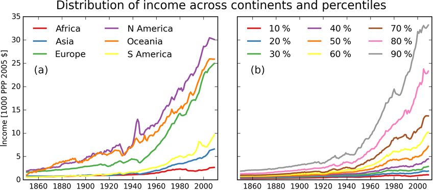
T. Geiger: Continuous national gross domestic product time series for 195 countries 849
ment models (IAMs) have generated GDP projections along
the SSP storylines. The associated national time series all
start in 2010. The historical data set we provide is designed
to allow for a smooth transition from historical time series to
the associated future projections. As such it can, e.g., be used
for transient climate impact model simulations covering the
historical period and future projections under different socio-
economic development pathways as described by the SSPs.
SSP projections are generally available at https://tntcat.
iiasa.ac.at/SspDb/dsd?Action=htmlpage&page=about. We
here use the OECD GDP data set (Dellink et al., 2017)
provided by the Inter-Sectoral Impact Model Intercom-
parison Project (ISIMIP), freely available at https://www.
isimip.org/gettingstarted/availability-input-data-isimip2b/
upon registration. This data set was directly provided by
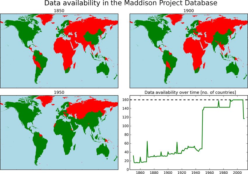
the OECD and is advantageous as it contains data on seven Figure 1. Illustration of data availability in the Maddison Project
additional countries. Note that one of these additional Database over time. Maps show the geographical distribution of
countries (Aruba, ABW) was excluded due to data issues. available data points for 3 selected years (1850, 1900, 1950), while
(The reported SSP GDP value for 2010 is a factor of 10 the plot displays the actual number of available countries over the
smaller than observational records.) full period. Countries are displayed using their current borders. We
only show data for those 160 countries that are explicitly named
in the Maddison Project Database; country group estimates lacking
2.1.4 Maddison Project national resolution are not shown (see Table 2 for details).
The Maddison Project resembles a cooperative effort to as-
semble historical national accounts (Bolt and van Zanden, History Database of the Global Environment (HYDE)
2014), continuing the ground-breaking work by the late An-
gus Maddison. The MPD is a freely available Excel spread- HYDE is developed under the authority of the Nether-
sheet (Maddison, 2016) that provides per capita income (in lands Environmental Assessment Agency and provides (grid-
1990 Geary–Khamis, G–K, dollars) for 184 countries and/or ded) time series of population and land use for the last
world regions between AD 1 and 2010 in varying time inter- 12 000 years (Klein Goldewijk et al., 2010, 2011). HYDE
vals. Since 1800 data have been provided annually, contain- provides national population data decennially up to 2000 and
ing however large fractions of missing values, in particular annually up to 2015. Where required we linearly interpolate
for the African continent, Western Asia and the former Soviet the data to derive annual distributions.
Union. The global missing value fraction is 61.8 % between
1800 and 2010. It steadily decreases to 51.7 % (36.9 %) when 2.3 Completing the Maddison Project Database
analyzing the data from 1850 (1900) onwards. After 1950,
when national accounts data were starting to be routinely col- The MPD provides income data on a national and supra-
lected, the missing value fraction drops to 8 %. The data are national level, where the supranational data represent
nearly complete since 1990 (missing value fraction: 3.6 %). population-weighted averages of national values (see Ta-
See Fig. 1 and the supplementary data in the DOI data archive ble 2). In addition, there exist three world region-specific
(Geiger and Frieler, 2018). groups of small countries (groups of 14 small European
We selected 1850 as the start year for our present work for countries, 21 Caribbean countries, and 24 South-East Asian
two reasons: first, coverage is somehow better than in 1800, countries) which lack national resolution; i.e., member coun-
and second, we can rely on available data points between tries are prescribed identical growth paths (see Table 2). In
1800 and 1849 for the purpose of interpolation rather than the following, each of the three country groups is treated like
extrapolation. an individual country with respect to replacement of missing
data.
2.2 Population data
Generally, gap filling is first done on the supranational
level and later gaps in national time series are filled by ac-
Parts of the GDP data sets (PWT and WDI) also provide na- counting for growth rates of either neighboring countries, the
tional population data to derive income. Whenever available associated supranational level, or the associated world region
we use the associated population estimates from the same the country belongs to.
source to derive income from GDP. However, to estimate na- In the following we present our gap-filling methodology,
tional GDP from the income data generated within the MPD first general steps and then for each world region in detail,
we use population estimates from the HYDE data set. starting with regions with the least missing values.
www.earth-syst-sci-data.net/10/847/2018/ Earth Syst. Sci. Data, 10, 847–856, 2018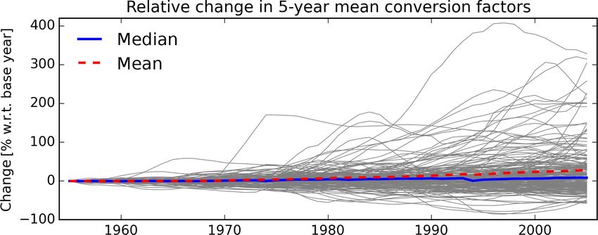
850                                      T. Geiger: Continuous national gross domestic product time series for 195 countries

Table 2. Overview of the world region-specific supranational country groups and the small country groups that lack national resolution, as
used within the Maddison Project Database.

                World region     Supranational group 1          Supranational group 2       Small country groups
                Europe           12 Western European (WE)       7 Eastern European (EE)     14 small European countries
                Latin America    8 Latin American (LA)          –                           21 Caribbean countries
                Asia             16 Eastern Asian (EA)          Western Asian (WA)          24 South-East Asian countries
                Africa           African total (AT)             –                           –

2.3.1   Preparatory steps                                              2.3.4    Latin America

As a first step we populate all missing data points in 1850,           Following the country grouping in the MPD, we generate
the initial year of our data product, by linear interpolation          a complete population-weighted average income time series
between the last available data point before 1850 and the first        for a group of eight large Latin American (LA) countries. To
one after 1850, ensuring that it is not more distant in time           do so, Peru and Mexico’s income is respectively extrapolated
than 1870. Next, and if available, we generate annual data             before 1870 and interpolated after 1870 based on the mean
by linear interpolation of data points between 1850, 1860,             growth of the seven remaining countries. Relative changes
and 1870. These preparatory steps reduce the missing value             in the LA time series are applied to estimate the income of
fraction from 51.7 to 48.5 %.                                          the remaining South American countries. The time series for
                                                                       the group of 21 Caribbean countries is linearly interpolated
                                                                       and then used to fill gaps in the remaining Caribbean and
2.3.2   Europe                                                         Central American countries, except for Jamaica and Cuba,
                                                                       whose time series is sufficiently dense to be interpolated in-
The preparatory steps completed the country-level data for             dividually.
most countries in Western Europe. These individual country-               Finally, the fraction of missing values is reduced to 29.7 %.
level data are then used to complete the time series for the
supranational group of 12 Western European (WE) coun-
tries by population-weighted mean income using HYDE’s                  2.3.5    Asia
national population data, as growth rates from the WE time
                                                                       Asia is separated into East and West Asia, reduced by the
series are used to approximate missing values for the country
                                                                       fraction that belonged to the former USSR.
group of 14 small European countries. Similarly, the United
                                                                          Where required relative income changes based on the lin-
Kingdom’s growth path is used to complete Ireland’s time
                                                                       early interpolated time series for a group of 16 Eastern Asian
series.
                                                                       (EA) countries are used to extrapolate individual country
   Next, gaps in the supranational group of seven Eastern Eu-
                                                                       data before 1870. Furthermore, data gaps for selected coun-
rope (EE) countries time series are linearly interpolated (in-
                                                                       tries with quite dense coverage (India, Japan, Indonesia (Java
cluding the time of World War 2) and then, starting in 1870,
                                                                       before 1880), Sri Lanka, and China) are filled by linear inter-
used to extrapolate individual country growth paths in East-
                                                                       polation on an individual basis. Using a step-wise procedure,
ern Europe back to 1850.
                                                                       we fill the EA time series after 1870 with the population-
   Relative changes in the former Yugoslavia’s time series
                                                                       weighted average income of all countries for which original
are used to extrapolate their temporary constituents back to
                                                                       data are available at any given time step. Relative changes in
1850, and to extrapolate Kosovo’s income between 1991 and
                                                                       the EA time series are then used to fill gaps in all remain-
2010. The same procedure is conducted for the constituents
                                                                       ing Eastern and South-East Asian countries, in particular to
of the former Czechoslovakia.
                                                                       complete the time series for the joint group of 24 South-East
   Relative EE changes prior to 1885 are used to complete the
                                                                       Asian countries. However, missing values for Bangladesh
former USSR time series. The relative changes in the USSR
                                                                       and Pakistan are estimated based on India’s relative changes.
time series are used to extrapolate income for all member
                                                                       Thereby, the fraction of missing values is reduced to 24.3 %.
countries of the USSR up to 1973, and to interpolate between
                                                                          In a second step, Western Asian countries including the
1973 and 1990. The fraction of missing values in the entire
                                                                       Gulf States are treated, where data availability is very lim-
data set thus decreases to 34.4 %.
                                                                       ited before 1950. Except for Turkey (former Ottoman Em-
                                                                       pire, complete data since 1923), relevant data points exist
2.3.3   North America, Australia, and New Zealand                      only for 1820, 1870, and 1913. To also include countries with
                                                                       completely missing data before 1950, we assume that the in-
The preparatory steps were sufficient to fill the respective           come of Israel is equal to West Bank/Gaza income in 1870
time series completely.                                                and 1913, and that the income of some Gulf States is equal

Earth Syst. Sci. Data, 10, 847–856, 2018                                                  www.earth-syst-sci-data.net/10/847/2018/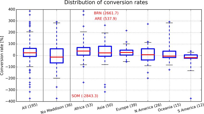
T. Geiger: Continuous national gross domestic product time series for 195 countries                                           851

to Iran’s income. For each country we linearly interpolate        rising conversion factors with time (see Fig. 3 below for a
the data until 1913, and again until 1950, except for Kuwait,     more detailed discussion). The income in 2005 PPP USD
Qatar, and the UAE. For those three countries we estimate in-     is determined from the income in 1990 GK USD by using
come growth to 1939 based on average income growth for all        the country-specific conversion factor (CF) for the respective
Western Asian (WA) countries and then linearly interpolate        base year:
each country individually between 1940 and 1950, thereby
ensuring that sharp income rises only occur after the discov-
ery of oil.                                                       Income (2005 PPP USD)
   Upon completing Asian time series the fraction of missing         = Income (1990 GK USD) · CF (base year) .
values is reduced to 19.5 %.

2.3.6    Africa
                                                                  To test for robustness the conversion factors are calculated
                                                                  for not only the earliest reporting year of PWT8.1, but also
The MPD contains only six countries with income data              for each of the first 5 years. If the five individual conversion
prior to 1950: Egypt, Tunisia, Morocco, Algeria, and South        factors significantly vary (fraction of standard deviation of
Africa/Cape Colony (all since 1820), and Ghana (since             the first five conversion factors and the first conversion factor
1870). Therefore, the African total (AT) population-weighted      larger than the iteratively derived threshold of 4 %), we use
average income prior to 1950 is only defined by six countries.    the 5-year mean conversion factor instead. In total, 78 out of
For historic and geographic reasons, we assume that those         195 countries require a mean conversion factor, while over-
countries define the upper income limit when extrapolating        lapping time series for 14 countries are so short that a mean
the remaining countries back in time. So if a country’s 1950      conversion factor cannot be determined. All conversion fac-
income is smaller than the six-country population-weighted        tors and the base year of matching are available in the Sup-
mean, the income fraction is used to define the scaled income     plement as well as supplementary data in the DOI archive
in 1913; otherwise, it is set equal to the six-country mean in    (Geiger and Frieler, 2018). Figure 2 provides an illustration
1913. Missing data between 1913 and 1950 are then interpo-        of the conversion factors, here shown as conversion rates in
lated according to scaled AT relative changes, while the bare     percent to highlight the symmetrical scattering around the
AT relative changes are used to extrapolate missing values        cross-country median, which is larger than unity, as expected,
from 1913 to 1850.                                                due to the transformation forward in time between 1990 and
                                                                  2005. The statistical distribution of conversion rates is shown
2.3.7    Summary
                                                                  for all 195 countries (left boxplot in Fig. 2), all 36 countries
                                                                  that do not appear specifically in the MPD but as country
Using all the steps described above, all missing values are       groups only (“no Maddison” boxplot in Fig. 2; see also Ta-
filled and a complete time series (1850–2010) is obtained for     ble 2), and separately for six different world regions. The out-
all countries listed within the MPD. This time series, reported   liers ARE (United Arab Emirates), BRN (Brunei), and SOM
in 1990 G–K dollars and matched with IS03 country codes,          (Somalia) are explicitly stated in Fig. 2, making their respec-
can be found in the DOI data archive (Geiger and Frieler,         tive converted time series before 1970 and 2010 rather un-
2018). Note that for some countries the reporting period ends     certain. A large fraction of relatively large conversion rates
in 2008; no extrapolation was done thereafter as more reli-       stems from those countries with no individual resolution in
able data from other sources are available for this period.       the MPD (“no Maddison” boxplot in Fig. 2) that are matched
                                                                  to PWT8.1 data using the respective country group data; see
2.4     Matching and time series conversion
                                                                  Table 2. In contrast to the other world regions, Europe and
                                                                  South America show rather small variations in conversion
Our final database is reported in PPP dollars referenced to       rates that are in line with the relatively dense data coverage
2005, the original unit of PWT8.1 and the SSPs. Conse-            within the MPD.
quently, data from the MPD, the WDI, and PWT9.0 require              Additional countries that are reported in the SSPs but not
conversion. As for the MPD, no official conversion factors        in PWT8.1 are included based on data first from PWT9.0
are available; time series of historic income from the MPD        and second from WDI, except for El Salvador (SLV) and
are scaled to systematically match PWT8.1 income data at          Zimbabwe (ZWE), where PWT9.0 data are chosen in place
the earliest reporting year of PWT8.1 data. This ensures that     of the available PWT8.1 due to known issues in the data
(1) time series for a large fraction of countries (18.5 %) with   set; see https://www.rug.nl/ggdc/docs/what_is_new_in_pwt_
no country-specific resolution in the MPD are assigned indi-      81.pdf for details. Conversion of PWT9.0 data between 2011
vidual growth paths as soon these data are available, (2) data    PPP USD and 2005 PPP USD values is conducted by us-
already provided in the finally desired currency unit (2005       ing the PWT-provided exchange rates (PWT abbreviation:
PPP USD) are used preferably, and (3) the risk of overes-         xr) and price levels of GDP (PWT abbreviation: pl_gdpo)
timation of values in the distant past is reduced because of      to yield the following PWT- and country-specific conversion

www.earth-syst-sci-data.net/10/847/2018/                                            Earth Syst. Sci. Data, 10, 847–856, 2018
852 T. Geiger: Continuous national gross domestic product time series for 195 countries
Figure 3. Base year dependent relative change in 5-year running-
mean conversion factors for all 181 countries (gray lines) for which
a 5-year mean can be determined. The cross-country mean (red-
dashed) and the median (blue-solid) conversion factor increase by
Figure 2. Statistical distribution of conversion rates used to convert 28.2 and 8.4 % between 1954 and 2005, respectively.
1990 GK USD to 2005 PPP USD. Most countries are close to the
cross-country median conversion rate (+23.3 %, red line in the left
boxplot), while SOM (Somalia), ARE (United Arab Emirates), and
BRN (Brunei) (stated in red; ARE, BRN, and SOM also appear in directly. An illustrative example of the matching procedure
the “all” boxplot, ARE additionally in the “no Maddison” boxplot) for four selected countries is displayed in Fig. 4; the match-
are clear outliers with respective conversion rates shown in paren- ing result for all 195 countries is shown in Fig. S1 in the
theses. Whiskers display the 5 to 95 % percentile range. Numbers in Supplement.
parentheses on the horizontal axis indicate the number of countries As mentioned above, there are several reasons why we
included in the respective boxplot.
use the earliest year of data availability for PWT8.1 data as
a base year for conversion, one of which being insufficient
factor CFPWT : coverage for many countries in the MPD. While this is a sen-
sible decision for most countries where conversion factors
CFPWT (2011 PPP USD → 2005 PPP USD) do not fluctuate rapidly over time, it can lead to distortions
= xr (2005) · pl_gdpo(2005)
xr (2011) · pl_gdpo(2011) .
for some countries as, e.g., hyperinflation, economic crisis,
or rapid economic growth may produce different conversion
For WDI data we use the provided PPP conversion table factors in different base years. In general, using earlier years
(Worldbank, 2017) and corrections for inflation based on the for matching results in more conservative estimates of past
USA GDP deflator (Worldbank, 2017) to yield the following income because mean and median conversion factors across
WDI- and country-specific conversion factor CFWDI : countries grow with time; see Fig. 3.
Figure 3 also illustrates that changes in country-specific
CFWDI (2011 PPP USD → 2005 PPP USD) conversion factors over time cluster at relatively low values,
= PPPconv (2005) PPPconv (2011) · GDPdefl (2011 → 2005) , while some countries show larger deviations and fluctuations
from the mean development. Table 3 therefore provides a
where GDPdefl ∼ 0.89 accounts for the price increase in the more detailed sensitivity analysis for 181 countries for which
USA economy of about 12 % between 2005 and 2011. Where at least 5 years of overlapping data exist. For more than 70 %
sufficient information was missing to convert between 2011 of the countries the change in conversion factors is smaller
and 2005 PPP USD, we either used the USA GDP deflator than 50 %, while almost 14 % of the countries show changes
only (for SLV, El Salvador, and ZWE, Zimbabwe), or used larger than 100 %. This sensitivity check provides useful in-
the conversion of a neighboring country (NRU, Nauru, in- formation about the uncertainty of past income estimates:
stead of KIR, Kiribati). North Korea (ISO3: PRK) is only users should keep in mind that income estimates are inher-
available in the MPD and is therefore excluded from the anal- ently uncertain not only due to reporting issues and lack of
ysis. data, but also due to currency conversion and their respective
In order to be consistent with SSP projections starting in change over time. Country-specific conversion factors over
2010, we truncate the observation-based time series in 2005 time are provided for selected countries in Fig. 4 and for all
and linearly interpolate from 2006 to 2009. Despite the fact countries in Fig. S1.
that we drop 4 years of observational data including the unan- In a next step we multiply income and population time se-
ticipated changes due to the global financial crisis (SSP prod- ries to obtain GDP time series. As for the income matching
ucts were produced many years prior to the financial crisis), between historical observations and SSP projections, popu-
we opted for this smooth procedure consistent with other lation estimates are truncated in 2005 and linearly interpo-
SSP-informed data sources to avoid large unphysical kinks lated to match SSP population projections in 2010. For al-
in the time series. Users that require more recent observa- most all countries the initial value of the SSP time series in
tional data are advised to rely on the underlying data sources 2010 and actually observed GDP values in 2010 only slightly
Earth Syst. Sci. Data, 10, 847–856, 2018 www.earth-syst-sci-data.net/10/847/2018/T. Geiger: Continuous national gross domestic product time series for 195 countries 853
Figure 4. Results of matched GDP per capita time series for Maddison, PWT, and OECD SSP2 data for selected countries: ARG: Argentina;
BDG: Bangladesh; USA: United States of America; ZAF: South Africa. Original Maddison data (blue, in 1990 GK USD) are matched to
PWT data (yellow, in 2005 PPP USD) using a country-specific base year and conversion factor, to obtain converted Maddison data (gray, in
2005 PPP USD). Between 2006 and 2009, PWT data are interpolated (red) to match OECD SSP2 projections (maroon) starting in 2010. The
sensitivity of the conversion factor over time is displayed to the right of each income time series. The black (red) point indicates whether
the selected conversion factor was chosen based on the first overlapping year (5-year mean), while the dark gray and light gray shaded areas
show the conversion factor min/max range for the first 5 overlapping years and for the 5-year running mean between the base year and 2005,
respectively.
deviate; see Figs. 4 and S1: only six countries show devia- Table 3. Changes in 5-year running-mean conversion factors be-
tions larger than 10 % (AZE, Azerbaijan, GNQ, Equatorial tween the country-specific base year and 2005 for all 181 countries
Guinea, PNG, Papua New Guinea, SLV, El Salvador, TLS, that have sufficient overlapping years of data. Where informative
Timor-Leste, ZWE, Zimbabwe). Even though the deviation the specific countries are listed with their respective ISO3 codes;
illustrated in Fig. 4 corresponds to income deviations only, italicized countries lack individual country resolution in the MPD.
it also reflects GDP differences well as the SSP income pro-
jections are the main source of deviations, mostly due to the Threshold No. of % of Selected list
in % countries countries of countries
already mentioned fact that SSP simulations were completed
(181)
before the financial crisis in 2008. However, Zimbabwe
shows a large discrepancy of about 70 % that is caused by ≤ ±5 2 1.1 HRV, UZB
differences in both income and population estimates. When ≤ ±10 14 7.7 –
using Zimbabwe’s time series for historical analysis only, we ≤ ±20 52 28.7 –
recommend truncation of the time series in 2005. Further- ≤ ±25 69 38.1 –
≤ ±50 127 70.2 –
more, for the following countries (Aruba, ABW, Antigua and
≤ ±100 156 86.2 –
Barbuda, ATG, Bermuda, BMU, Dominica, DMA, Federated > ±100 25 13.8 –
States of Micronesia, FSM, Grenada, GRD, Kiribati, KIR, > ±200 10 5.5 ABW, ARG, GAB,
Saint Kitts and Nevis, KNA, Marshall Islands, MHL, Nauru, GRD, IRQ, KNA,
NRU, Seychelles, SYC, Tuvalu, TUV), no GDP projections KWT, MAC, MDV,
exist in the OECD database. We therefore used the observa- QAT
tional data from our reconstruction up to 2009.
For some small countries HYDE data have missing
population values prior to certain years (Bermuda, BMU, valu, TUV < 1960). Therefore, the corresponding GDP time
Macao, MAC, Maldives, MDV < 1970; Federated States of series contains missing values for this period.
Micronesia, FSM, Kiribati, KIR, Marshall Islands, MHL,
Nauru, NRU, French Polynesia, PYF, Seychelles, SYC, Tu-
www.earth-syst-sci-data.net/10/847/2018/ Earth Syst. Sci. Data, 10, 847–856, 2018854 T. Geiger: Continuous national gross domestic product time series for 195 countries
3 Data availability
We provide three different primary data sets, a data de-
scription file, and two supplementary data sets in the online
archive at https://doi.org/10.5880/pik.2017.003.
1. A continuous table of global income data (in original
1990 G–K USD) based on the MPD for 160 individual
countries and 3 groups of countries from 1850 to 2010.
2. A continuous and consistent table of global income
Figure 5. Distribution of population-weighted income over time
data (in 2005 PPP USD) for 195 countries based on
across continents (a) and percentiles (b) that can be analyzed for,
the merged MPD and PWT8.1 data and extended using e.g., income inequality or other distributional effects. Percentiles
PWT9.0 and WDI data from 1850 to 2009, and con- rank the number of countries by average national income.
sistent with OECD SSP2 income projections starting in
2010.
3. A continuous and consistent table of global GDP
data (in 2005 PPP USD) for 195 countries based on with various techniques to replace missing values. Our main
the merged MPD and PWT8.1 data, extended using assumption is that geographically close countries have ob-
PWT9.1 and WDI data, and consistent with OECD served similar growth paths over the last 150–200 years, such
SSP2 GDP projections starting in 2010. that we can use neighboring (groups of) countries to estimate
missing data. This assumption strongly depends on many po-
The second data set is illustrated in Fig. 5, showing the litical, economical, and societal aspects (e.g., the economic
population-weighted income distribution across continents system, the membership in alliances, the occurrence of wars,
and percentiles. the colonial background, and many more) that, however,
Furthermore, we provide two supplementary data sets. were not considered in our work. While rather exhaustive
1. A mask table complementing the first primary data set data exist for Western European countries, these limitations
indicating which of the data points are original values might be less of a problem than for most African countries.
and which are estimated based on our present method- As a consequence, one should treat the data with care and
ology, and used to generate Fig. 1. allow for uncertainties, in particular where data coverage is
limited or almost non-existent.
2. A table of conversion factors (1990 GK USD to 2005 Another limitation arises due to different units: the origi-
PPP USD) also indicating the data source used for nal MPD is measured in 1990 GK USD, while all other data
matching and the methodology used for conversion, and sets use PPP equivalents in either 2005 or 2011 USD. The
used to generate Fig. 2. required PPP transformation can lead to underestimation or
overestimation of economic figures, in particular further back
All data sets are provided in “csv” format and are freely in time. As mentioned above for Brunei (discovery of fos-
available at https://doi.org/10.5880/pik.2018.010. Please also sil fuels) and Somalia (ethnic conflict and civil war), large
consult the data description file for additional information on conversion factors are due to rapid changes in a country’s in-
the data set. come over a short period of time that can deteriorate the PPP
conversion. However, as currently there exists no reliable so-
4 Discussion and conclusion lution to circumvent this conversion problem, one has to in-
terpret transformed data with caution. For example, countries
In conclusion, we provide a continuous time series for per that mainly depend on fossil-fuel exports had rapid income
capita income and GDP between 1850 and 2009 for 195 jumps in the not so distant past that can overestimate their
countries. The foundation of our work is the income data income before oil discovery. For this reason we also provide
set maintained by the Maddison Project, which is completed the interpolated MPD in original 1990 GK USD. In addition
using various interpolation and extrapolation techniques and to this, the choice of a specific base year for currency conver-
harmonized with economic data from the Penn World Tables. sion introduces additional uncertainty about past estimates.
The main objective is to provide a continuous economic time For several reasons discussed above, we here systematically
series that is readily applicable across disciplines and by non- rely on a conversion factor defined at the earliest possible
experts in the field. The methodology applied is rather simple time. While this provides a rather conservative estimate of
and comes with several limitations and caveats. historical income in general, a different base year for con-
As we do not devise new historic economic figures our- version can yield large differences for some countries, as our
selves, we are bound to existing data only that are combined sensitivity assessment has shown.
Earth Syst. Sci. Data, 10, 847–856, 2018 www.earth-syst-sci-data.net/10/847/2018/T. Geiger: Continuous national gross domestic product time series for 195 countries 855
Another problem arises due to shifting national borders, Competing interests. The author declares that he has no conflict
and the formation of new and disappearance of old nations: of interest.
the data sets only reflect the current political map defined
by the list of countries available in the PWT8.1 database.
To circumvent but not fully exclude this problem, we work Acknowledgements. We wish to thank Johannes Gütschow for
with per capita income time series until the very last moment his valuable comments on the generation of this data set and Katja
that are then multiplied by historical population data to gen- Frieler for her helpful remarks to improve the manuscript. We also
thank Jutta Bolt for advice on the Maddison Project Database. We
erate GDP estimates. The income data are here provided as
further thank Kirsten Elger from GFZ Data Services for invaluable
well such that the inclined user can generate GDP time series
support in creating the DOI data archive.
for a different political map himself. For consistency reasons This work was funded through the framework of the Leibniz
population and income estimates are selected from identical Competition (SAW-2013-PIK-5 and SAW-2016-PIK-1).
sources, except for the MPD, where HYDE data are used.
However, when merging different time series, inconsisten- Edited by: David Carlson
cies arise due to different country definitions, e.g., as is the Reviewed by: two anonymous referees
case for countries in the former Yugoslavia or for the transi-
tion between historical data and SSP projections. To reduce
the inconsistencies to a minimum we rely on the country def-
References
initions in PWT8.1 and adjust the other sources to it. Regard-
ing the former Yugoslavia, we split the population estimates Baier, S. L., Dwyer, G. P., and Tamura, R.: How Important Are Cap-
for missing time periods for SCG (Serbia and Montenegro) ital and Total Factor Productivity for Economic Growth?, Econ.
into Serbian (SER) and Montenegrin (MNE) parts based on Inq., 44, 23–49, https://doi.org/10.1093/ei/cbj003, 2002.
reported population ratios from 1990. Further, the population Bolt, J. and van Zanden, J. L.: The Maddison Project: collabora-
of Kosovo (KSV) was added to Serbia (SER) to match with tive research on historical national accounts, Econ. Hist. Rev.,
the PWT’s estimates. A similar procedure was followed for 67, 627–651, https://doi.org/10.1111/1468-0289.12032, 2014.
the respective population of Israel (ISR) and Palestine (PSE) Deaton, A. and Heston, A.: Understanding PPPs and PPP-
prior to 1950 and 1969, respectively: reported population ra- based National Accounts, Am. Econ. J.-Macroecon., 2, 1–35,
https://doi.org/10.1257/mac.2.4.1, 2010.
tios were used to estimate a single country’s population fur-
Dellink, R., Chateau, J., Lanzi, E., and Magné, B.: Long-
ther back in time. No further adjustment was necessary for
term economic growth projections in the Shared Socioe-
the other world regions. conomic Pathways, Global Environ. Chang., 42, 200–214,
Furthermore and as mentioned above, historical popula- https://doi.org/10.1016/j.gloenvcha.2015.06.004, 2017.
tion estimates are unavailable for some small countries, mak- Feenstra, R. C., Inklaar, R., and Timmer, M. P.: The Next Genera-
ing the GDP time series incomplete. tion of the Penn World Table, Am. Econ. Rev., 105, 3150–3182,
Despite these shortcomings and uncertainties, this new https://doi.org/10.1257/aer.20130954, 2015.
data set will broaden the applicability of historic estimates Frieler, K., Lange, S., Piontek, F., Reyer, C. P. O., Schewe, J.,
of economic activity, e.g., in the field of climate impact re- Warszawski, L., Zhao, F., Chini, L., Denvil, S., Emanuel, K.,
search in order to facilitate impact simulations on centennial Geiger, T., Halladay, K., Hurtt, G., Mengel, M., Murakami, D.,
timescales (Frieler et al., 2017). It further provides the op- Ostberg, S., Popp, A., Riva, R., Stevanovic, M., Suzuki, T.,
Volkholz, J., Burke, E., Ciais, P., Ebi, K., Eddy, T. D., Elliott, J.,
portunity to generate gridded GDP distributions for the past
Galbraith, E., Gosling, S. N., Hattermann, F., Hickler, T., Hinkel,
based on recent downscaling initiatives (Geiger et al., 2017;
J., Hof, C., Huber, V., Jägermeyr, J., Krysanova, V., Marcé, R.,
Murakami and Yamagata, 2017). Moreover, the increased re- Müller Schmied, H., Mouratiadou, I., Pierson, D., Tittensor, D.
search interest in past GDP data will provide valuable feed- P., Vautard, R., van Vliet, M., Biber, M. F., Betts, R. A., Bodirsky,
back to the historians and economists working in this field B. L., Deryng, D., Frolking, S., Jones, C. D., Lotze, H. K., Lotze-
and might stimulate further advances. These advances are ex- Campen, H., Sahajpal, R., Thonicke, K., Tian, H., and Yamagata,
pected to improve this current data set further. Y.: Assessing the impacts of 1.5 ◦ C global warming – simula-
tion protocol of the Inter-Sectoral Impact Model Intercompar-
ison Project (ISIMIP2b), Geosci. Model Dev., 10, 4321–4345,
The Supplement related to this article is available online https://doi.org/10.5194/gmd-10-4321-2017, 2017.
at https://doi.org/10.5194/essd-10-847-2018-supplement. Geiger, T. and Frieler, K.: Continuous national Gross Domestic
Product (GDP) time series for 195 countries: past observations
(1850–2005) harmonized with future projections according the
Shared Socio-economic Pathways (2006–2100), V. 2.0, Potsdam
Institute for Climate Impact Research by GFZ Data Services,
Author contributions. TG created and analyzed the data set and
https://doi.org/10.5880/pik.2018.010, 2018.
wrote the paper.
Geiger, T., Murakami, D., Frieler, K., and Yamagata, Y.: Spatially-
explicit Gross Cell Product (GCP) time series: past observa-
tions (1850–2000) harmonized with future projections according
www.earth-syst-sci-data.net/10/847/2018/ Earth Syst. Sci. Data, 10, 847–856, 2018856 T. Geiger: Continuous national gross domestic product time series for 195 countries to the Shared Socioeconomic Pathways (2010–2100), Potsdam Maddison, A.: Contours of the world economy, 1–2030 AD: es- Institute for Climate Impact Research by GFZ Data Services, says in macro-economic history, Oxford University Press, Ox- https://doi.org/10.5880/PIK.2017.007, 2017. ford, 2007. Geiger, T., Frieler, K., and Bresch, D. N.: A global historical data set Maddison, A.: Maddison Project, available at: http://www.ggdc. of tropical cyclone exposure (TCE-DAT), Earth Syst. Sci. Data, net/maddison/maddison-project/data.htm, last access: 25 Octo- 10, 185–194, https://doi.org/10.5194/essd-10-185-2018, 2018. ber 2016. Gennaioli, N., and La Porta, R.: Human capital and Mitchel, B. R.: International Historical Statistics, Palgrave Macmil- regional development, Q. J. Econ., 128, 105–164, lan, London, UK, 2003. https://doi.org/10.1093/qje/qjs050, 2013. Murakami, D. and Yamagata, Y.: Estimation of gridded population Inklaar, R. and Rao, D. S. P.: Cross-Country Income Lev- and GDP scenarios with spatially explicit statistical downscal- els over Time: Did the Developing World Suddenly Be- ing, Environ. Res. Lett., available at: https://arxiv.org/abs/1610. come Much Richer?, Am. Econ. J. Macroecon., 9, 265–290, 09041, under review, 2017. https://doi.org/10.1257/mac.20150155, 2017. O’Neill, B. C., Kriegler, E., Ebi, K. L., Kemp-Benedict, E., Riahi, Klein Goldewijk, K., Beusen, A., and Janssen, P.: Long-term dy- K., Rothman, D. S.., van Ruijven, B. J., van Vuuren, D. P., Birk- namic modeling of global population and built-up area in a spa- mann, J., Kok, K., Levy, M., and Solecki, W.: The roads ahead: tially explicit way: HYDE 3.1, The Holocene, 20, 565–573, Narratives for shared socioeconomic pathways describing world https://doi.org/10.1177/0959683609356587, 2010. futures in the 21st century, Global Environ. Chang., 42, 169–180, Klein Goldewijk, K., Beusen, A., Van Drecht, G., and De Vos, https://doi.org/10.1016/j.gloenvcha.2015.01.004, 2017. M.: The HYDE 3.1 spatially explicit database of human-induced Speich Chasse, D.: Die Erfindung des Bruttosozialprodukts: globale global land-use change over the past 12,000 years, Global Ungleichheit in der Wissensgeschichte der Oekonomie, Vanden- Ecol. Biogeogr., 20, 73–86, https://doi.org/10.1111/j.1466- hock & Ruprecht, Göttingen, 2013. 8238.2010.00587.x, 2011. Worldbank: World Development Indicators, available at: http://data. Kousky, C.: Informing climate adaptation: A review of the eco- worldbank.org/, last access: 11 January 2017. nomic costs of natural disasters, Energy Econ., 46, 576–592, https://doi.org/10.1016/j.eneco.2013.09.029, 2013. Earth Syst. Sci. Data, 10, 847–856, 2018 www.earth-syst-sci-data.net/10/847/2018/
You can also read