Machine Learning Approach to Classify Rain Type Based on Thies Disdrometers and Cloud Observations - MDPI
←
→
Page content transcription
If your browser does not render page correctly, please read the page content below
atmosphere
Article
Machine Learning Approach to Classify Rain Type
Based on Thies Disdrometers and Cloud Observations
Wael Ghada 1, *, Nicole Estrella 1 and Annette Menzel 1,2
 1   Department of Ecology and Ecosystem Management, Technical University of Munich,
     Hans-Carl-von-Carlowitz-Platz 2, D-85354 Freising, Germany; estrella@wzw.tum.de (N.E.);
     amenzel@wzw.tum.de (A.M.)
 2   Institute for Advanced Study, Technical University of Munich, Lichtenbergstraße 2a, D-85748 Garching,
     Germany
 *   Correspondence: ghada@wzw.tum.de; Tel.: +49-81-6171-4743

 Received: 24 April 2019; Accepted: 4 May 2019; Published: 7 May 2019

 Abstract: Rain microstructure parameters assessed by disdrometers are commonly used to classify
 rain into convective and stratiform. However, different types of disdrometer result in different values
 for these parameters. This in turn potentially deteriorates the quality of rain type classifications.
 Thies disdrometer measurements at two sites in Bavaria in southern Germany were combined with
 cloud observations to construct a set of clear convective and stratiform intervals. This reference
 dataset was used to study the performance of classification methods from the literature based on the
 rain microstructure. We also explored the possibility of improving the performance of these methods
 by tuning the decision boundary. We further identified highly discriminant rain microstructure
 parameters and used these parameters in five machine-learning classification models. Our results
 confirm the potential of achieving high classification performance by applying the concepts of machine
 learning compared to already available methods. Machine-learning classification methods provide
 a concrete and flexible procedure that is applicable regardless of the geographical location or the
 device. The suggested procedure for classifying rain types is recommended prior to studying rain
 microstructure variability or any attempts at improving radar estimations of rain intensity.

 Keywords: convective; stratiform; rain microstructure; Thies; disdrometer; classification;
 machine learning

1. Introduction
     Different precipitation droplet growth mechanisms lead to the different properties of convective
and stratiform rain [1–3]. This is due to the vertical development of convective clouds in contrast
to the more horizontal development of stratiform clouds [4]. An accurate classification of rain types
has the potential to improve radar estimations of the rain rate [5]. Equally importantly, it fosters the
development of global climate and circulation models [1,6,7]. In addition, it is an important preliminary
step to investigating variations of rain properties with general weather conditions [8].
     A simple and widely used rain classification method was proposed by Bringi et al. [9], where
a threshold of the rain intensity and its standard deviation over 10 successive minutes are used to
separate convective and stratiform intervals. Llasat [10] also classified rain using a rain intensity
threshold for different time intervals. Such methods are prone to misclassification [11]; however,
they are applicable independent of the instrument type. Another classification approach is based on
cloud observations [12–14]. Convective rain is expected when cumulus and cumulonimbus clouds are
observed, while nimbus and nimbostratus clouds produce stratiform rain. Rulfová and Kyselý [15] used
cloud types in combination with synoptic weather state reports for this purpose. Other methods rely on

Atmosphere 2019, 10, 251; doi:10.3390/atmos10050251                          www.mdpi.com/journal/atmosphere
Atmosphere 2019, 10, 251                                                                                 2 of 18

the availability of wind profiler [16] and radar [17–19] data, or satellite images [20–22]. These methods
classify the rain type by identifying patterns in the vertical wind velocity, the spatial and temporal
extension of the detected clouds, the reflectivity values and their variations, and the existence of a
bright band and its thickness. Radars and satellites have the advantage of wide coverage, but usually
assume specific drop size distribution (DSD) models derived by disdrometers.
      Just two decades after Yuter and Houze [23] questioned the accuracy of rain microstructure
techniques for rain type classification, Thurai et al. [24] concluded that “rain DSD classification is sound.”
Within this period, many classification methods were proposed relying on rain DSDs as provided by
different types of disdrometers. Each method provides a classification boundary based on a pair of
parameters, such as the rain rate with the slope parameter (R–Λ), the rain rate with the intercept parameter
(R–N0) [25], the slope with the shape parameter (Λ–µ) [26], the intercept with the slope parameter
(N0–Λ) [27], or the median drop diameter with the log normalized concentration (N0–logNw) [28].
      Despite the availability of all these methods, rain classification remains challenging, especially
because these classes are not mutually exclusive [6]. The successful use of one classification method for
one case study does not imply repetition in other cases where different climate conditions exist [26,29].
It might also be incorrect to apply a method that has been specifically developed for one type of
disdrometer to the measurements of another type of disdrometer [11]. For example, You et al. [30]
adjusted the method proposed by Bringi et al. [28] for a specific region (Korea) and a specific disdrometer
device (PARSIVEL). To improve the classification accuracy, Bukovčić et al. [11] proposed using a
Bayesian approach with four parameters. Such an approach requires the availability of vertical wind
speed measurements or cloud type observations to construct a prior classification.
      The German Meteorological Service DWD (Deutscher Wetterdienst) operates a large network
of Thies disdrometers across Germany for radar calibration and precipitation classification [31].
To adequately investigate rain microstructure variation using Thies disdrometers, an accurate method
for rain type classification is needed. However, no method exists that is specifically designed to classify
the rain type based on Thies disdrometers because most available methods were developed using
impact disdrometers or two-dimensional video disdrometers (2DVD). Thies disdrometers are low-cost
easy-maintenance devices. They are well suited to construct long-term climatological radar algorithms
with performances comparable to more accurate devices such as 2DVD [32]. Nevertheless, even
laser disdrometers that use the same detection principle have different designs, minimum sensitivity
thresholds, drop counting velocity and size ranges, and internal correction algorithms. Consequently,
bulk precipitation parameters, such as rain intensity, radar reflectivity, and kinetic energy, are significantly
different when measured by a Thies disdrometer compared to PARSIVEL [33]. These parameters are
also used in the different rain type classification methods, and thus the following questions must
be asked.
•    How do classification methods designed for other disdrometer types perform when applied to
     Thies disdrometer measurements?
•    Can we achieve better classification performance by tuning the decision boundary for each method?
•    Which rain microstructure parameters are superior as rain type classifiers?
•    Do machine-learning techniques support a better classification?
     We aim to examine the performances of the available methods and their parameters.
These parameters will then be used to construct a classification method that should be suitable
for Thies disdrometers. The developed method will be needed in future studies to investigate the
spatial and temporal rain microstructure variations across Bavaria and Germany.

2. Materials and Methods

2.1. Data Sources and Tools
    We used cloud observations and measurements of rain DSDs by Thies disdrometers. Cloud
observations were obtained from the DWD’s Climate Data Center [34]. Disdrometer data were provided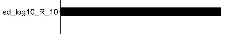
Atmosphere 2019, 10, 251                                                                              3 of 18

upon request directly from the DWD for two locations: Fürstenzell at 48.545146◦ N 13.353054◦ E
476.4 m ASL (hereafter FUR) and Regensburg at 49.042357◦ N 12.102053◦ E 365.4 m ASL (hereafter
REG). The availability of both cloud observations and DSD data limited the spatial and temporal extent
of the study. Simultaneous measurements and observation records were available between July 2013
and August 2014 at FUR and between July 2013 and January 2014 at REG.
     Data from FUR were used to test the performance of the existing classification methods and
to re-adjust the decision boundaries of these methods and improve their performance. These data
also served as a training set for constructing new predictive models. This included identifying the
most important predictors of rain type, constructing and training the models, and then testing their
performance by means of cross validation with 200 repetitions of stratified sampling.
     The REG data were used for testing the newly suggested models. This included the adjusted
models from the literature and the new predictive models, which were trained using the first dataset.
     For data handling, calculations, feature selection, model training, performance estimation, and
visual and statistical results, we used R [35], RStudio [36], and the reader [37], dplyr [38], reshape2 [39],
lubridate [40], stringr [41], ggplot2 [42], cowplot [43], caret [44], e1071 [45], doSNOW [46], zoo [47],
MASS [48], corrplot [49], and pROC [50] packages.

2.2. Cloud Observations
      According to the World Meteorological Organization (WMO), clouds are classified into ten genera
(hereafter types). These types can be further classified into species and varieties [51]. Cloud types
have been used to classify precipitation type [12–14]. Hourly observations of the cloud types are
available for both locations for up to four layers. Possible cloud types and the corresponding expected
rain type are provided in Table 1. Convective rain is believed to correspond to convective cloud
types (cumulus and cumulonimbus), while stratiform rain corresponds to stratiform cloud types
(stratus and nimbostratus) [12]. It is possible for several cloud types to be observed at the same time.
Such cases might produce mixed rain properties; therefore, these cases were discarded. All cloud data
have been recorded by trained staff, which still leaves (although reduced) chances for human errors.
However, DWD marks this data with the third quality level. This means that the data went through a
completeness check, climatological consistency check, time consistency check, internal consistency
check and spatial consistency check [52].

                           Table 1. Cloud types and their associated expected rain type.

                           Cloud Type (Genera)      Abbreviation      Expected Rain Type
                                  Cirrus                CI                     -
                              Cirrocumulus              CC                     -
                               Cirrostratus             CS                     -
                              Altocumulus               AC                     -
                               Altostratus              AS                     -
                              Nimbostratus              NS                Stratiform
                             Stratocumulus              SC                     -
                                 Stratus                ST                Stratiform
                                Cumulus                 CU                Convective
                             Cumulonimbus               CB                Convective

2.3. Thies Disdrometer and Extraction of Rain DSD
     Thies disdrometers provide the current weather state in addition to a number of precipitation
parameters such as the rain intensity and reflectivity with a high temporal resolution (1 min in our
case). However, the most relevant output in our case is the raw representation of the particle size
and velocity distribution. This is provided via the number of particles that fall within the limits of
22 particle size and 20 velocity ranges. The measurement principal is based on the reduction of the
power of a light beam that is transmitted from one end of the disdrometer to the other. The magnitude
and time of this reduction determine the size and velocity of the passing particle [53].
Atmosphere 2019, 10, 251 4 of 18
Specific filtering steps are needed prior to the calculation of the rain parameters. The process
proposed by Friedrich et al. [54], and additional steps performed by Ghada et al. [8], were used to
remove intervals with very high wind speed, snow, hail, frozen rain, graupel, intervals with very
low rain intensity (R < 0.1 mm/h), margin fallers, unrealistically large drops, and the splashing effect.
Consequently, the filtered rain data set contains 22,592 min at FUR and 4585 min at REG.
Table 2 provides a list of parameters that were calculated from the Thies measurements of the rain
DSD and rain velocity distribution. This list is the result of a literature survey of the potential predictors
of the rain type. Each reference contains either an equation to calculate the corresponding parameter or
the motivation for the use of the corresponding parameter. All these parameters can be obtained from
the rain DSD provided by a Thies disdrometer. Some parameters are acquired with different equations
according to different references (e.g., Lambda_TS, Lambda_Ca06, and Lambda_Ca08). These are
marked with the appropriate reference.
Atmosphere 2019, 10, x FOR PEER REVIEW 5 of 19
Table 2. Drop size distribution parameters as potential rain type classifiers.
Table 2. Drop size distribution parameters as potential rain type classifiers.
Abbreviation Unit Parameter Name and Relevant Reference 1
Abbreviation Unit Parameter Name and Relevant Reference
1
R R mm·h−1 mm∙h−1 rain intensity[8][8]
rain intensity
Z Z dBZ dBZ reflectivity[8][8]
reflectivity
Dm Dm mm mm mass
mass weighted diameter
weighted diameter [55]
[55]
D0 D0 mm mm median volumediameter
median volume diameter[56][56]
sd_D sd_D mm mm instantaneous
instantaneous (1(1 min) standarddeviation
min) standard deviationof of drop
drop sizesize
[2] [2]
sd_V sd_V m·h−1 m∙h−1 instantaneousstandard
instantaneous standard deviation
deviationofof drop
dropvelocities [2] [2]
velocities
Nt Nt −3
drop·mdrop∙m −3 totalnumber
total number of of drops
dropsper percubic meter
cubic meter[57][57]
Nw_Tes Nw_Tes −1
mm ·m mm−3−1∙m−3 normalized number
normalized numberofofdropsdrops[58]
[58]
Nw_Br Nw_Br mm−1 ·m mm−3−1∙m−3 normalized number
normalized numberofofdropsdrops[28]
[28]
logNw logNw Nw:
Nw: mm ·m −1 mm −3−1∙m−3 logNw =
logNw = log (NW_Br)
log1010 (NW_Br)
D0_Nt 3mm.m3−1 ∙drop−1 D0/Nt [59]
D0_Nt mm.m ·drop −1 D0/Nt [59]
Lambda_TS −1 mm slope of fitted gamma distribution [25]
Lambda_TS mm slope of fitted gamma distribution [25]
logLambda Lambda: mm−1 logLambda = log10(Lambda_TS) [25]
logLambda Lambda: mm−1 logLambda = log10 (Lambda_TS) [25]
mu_TS ‐ shape of fitted gamma distribution [25]
mu_TS - shape of fitted gamma distribution [25]
N0_TS −1−m
mm−1−m
−3
∙m−3 intercept of fitted gamma distribution [25]
N0_TS mm ·m
N0_TS: intercept of fitted gamma distribution [25]
logN0 logN0N0_TS: mmmm −1−m ·m−3
−1−m∙m−3
logN0 =
logN0 = log (N0_TS)
log1010 (N0_TS) [25]
[25]
Lambda_Ca06Lambda_Ca06 mm−1 mm−1 slope
slope of fitted gamma distribution [26][26]
of fitted gamma distribution
mu_Ca06 mu_Ca06 - ‐ shape
shapeof
of fitted gammadistribution
fitted gamma distribution [26][26]
N0_Ca06 −1−m ·m−1−m
−3 intercept
N0_Ca06 mm mm ∙m−3 intercept of
of fitted gammadistribution
fitted gamma distribution [26][26]
Lambda_Ca08Lambda_Ca08 mm−1 mm−1 slope
slopeof
of fitted gammadistribution
fitted gamma distribution [27][27]
N0_Ca08 N0_Ca08 mm−1−m −3 ∙m−3
·m−1−m
mm intercept
intercept of
of fitted gammadistribution
fitted gamma distribution [27][27]
Nt_4R Nt_4R (Drop·m −3 )0.25 −3)0.25
(Drop∙m 4th root
rootofofNtNt[11]
[11]
sd_R_10 sd_R_10 mm·h−1 mm∙h−1
sd_Dm_10 sd_Dm_10 mm mm
sd_D0_10 sd_D0_10 mm mm
sd_Nt_10 sd_Nt_10 drop drop
sd_R_30 sd_R_30 mm·h−1 mm∙h−1
sd_XX_YY:
sd_XX_YY: standarddeviations
standard deviations of
of XX
XXover
overYY
YY
sd_Dm_30 sd_Dm_30 mm mm minutes[11]
minutes [11]
sd_D0_30
sd_D0_30 mm mm
sd_Nt_30 drop
sd_Nt_30 drop
sd_log10(Nt)_30 ‐
sd_log10 (Nt)_30 -
sd_log10(R)_30 ‐
sd_log10 (R)_30 -
sd_log10(Nt)_10 ‐
sd_log10 (Nt)_10 -
sd_log10 (R)_10sd_log10(R)_10 - ‐
1 The Thewas
1
parameter parameter
used was used
in (or in (or motivated
motivated by)associated
by) the the associated reference.
reference.
2.4. Prior Rain Type Classification
2.4. Prior Rain Type Classification
Clearly separated convective and stratiform samples of rain are needed to evaluate the
performance of the classification methods. We relied in the first step on the simple and widely used
Clearly separated convective and stratiform samples of rain are needed to evaluate the performance
method of Bringi et al. [9], where rain is considered to be convective when the standard deviation of
of the classificationrain
methods. We
intensity over relied
five in the
consecutive firstintervals
two‐min step on the simple
exceeds 1.5 mm/h and
or whenwidely
the rainused method of
intensity
exceeds 10 mm/h. There is a risk of misclassification for weak convective and strong stratiform events.
Bringi et al. [9], where rain is considered to be convective when the standard deviation of rain intensity
Therefore, in a second step, we restricted the convective intervals to instances that corresponded to
over five consecutive two-min
convective intervals
cloud types and exceeds 1.5events
the stratiform mm/h or when
to those the rainto intensity
corresponding exceeds
stratiform clouds. This 10 mm/h.
There is a risk of misclassification for weak
step removed all intervals whereconvective
a combinationand strong stratiform
of convective and stratiformevents. Therefore,
cloud types was in a
observed, and intervals where none of the four relevant cloud types were observed (nimbostratus,
second step, we restricted the convective intervals to instances that corresponded to convective cloud
stratus, cumulus, and cumulonimbus). Events were defined by a minimum inter‐event time of 15 min
where the rain intensity did not exceed 0.1 mm/h.Atmosphere 2019, 10, 251 5 of 18
types and the stratiform events to those corresponding to stratiform clouds. This step removed all
intervals where a combination of convective and stratiform cloud types was observed, and intervals
Atmosphere
where none 2019,
of 10,
thex FOR
fourPEER REVIEW
relevant cloud types were observed (nimbostratus, stratus, cumulus, 6 of and
19
cumulonimbus). Events were defined by a minimum inter-event time of 15 min where the rain intensity
Figures 1 and 2 display examples from the reference dataset. All events in Figure 1 occurred
didAtmosphere
not exceed 2019, 0.1
10, xmm/h.
FOR PEER REVIEW 6 of 19
while a convective cloud type was observed. We are only interested in instances that show high rain
Figures 1 and 2 display examples from the reference dataset. All events in Figure 1 occurred
intensities or sudden 2 variations in the intensity. theTherefore, intervals where the convective 1signal was
while aFigures
convective1 and clouddisplay examples
type was from We
observed. reference
are dataset. All
only interested events
in instances in Figure
that show occurred
high rain
weak were filtered
while a convective out (blue points). In the case of stratiform clouds (Figure 2), when an event
intensities or suddencloud type was
variations in observed. We are
the intensity. only interested
Therefore, in instances
intervals where the thatconvective
show high rain signal
contained
intensities even
or one interval
sudden that was
variations in classified
the intensity. asTherefore,
convectiveintervals
rain by the classification
where the method
convective of Bringi
signal
was weak were filtered out (blue points). In the case of stratiform clouds (Figure 2), when anwas
event
et al. [9],
weak the entire
were filtered event
out was removed
(blue points).because
In the it might
case of be an indication
stratiform clouds of(Figure
a convective cell embedded
2), when an event of
contained
within even one
a stratiform interval that was classified as convective rain by the classification method
contained even onecloud. These
interval that events are marked
was classified with an asterisk
as convective rain by in
thethe top left corner
classification of each
method panel.
of Bringi
Bringi
The et al. [9],
filtered the entire
dataset with eventclassification
prior was removed of because
rain type it might be
consisted of an
7260indication
min (674 of a convective
min) of stratiformcell
et al. [9], the entire event was removed because it might be an indication of a convective cell embedded
embedded
(convective) within a stratiform
rain at cloud.
FUR and cloud.
406eventsThese
min (83 min)events are marked
of stratiform with an
(convective) asterisk in the top left corner of
within a stratiform These are marked with an asterisk in therain
topat REG.
left corner of each panel.
each panel. The filtered dataset with prior classification of rain type consisted of 7260 min (674 min) of
The filtered dataset with prior classification of rain type consisted of 7260 min (674 min) of stratiform
stratiform (convective) rain at FUR and 406 min (83 min) of stratiform (convective) rain at REG.
(convective) rain at FUR and 406 min (83 min) of stratiform (convective) rain at REG.
Figure 1. Rain intensity variations for selected events with convective clouds at Fürstenzell. Rain
intervals classified as stratiform by Bringi et al. [9] (blue points) were removed from the reference
Figure 1. Rain intensity variations for selected events with convective clouds at Fürstenzell. Rain
dataset.
Figure classified
1. Rain intensity variations for et
selected events with were
convective clouds
intervals as stratiform by Bringi al. [9] (blue points) removed fromatthe
Fürstenzell. Rain
reference dataset.
intervals classified as stratiform by Bringi et al. [9] (blue points) were removed from the reference
dataset.
Figure 2. Rain intensity variation for selected events with stratiform clouds at Fürstenzell. Rain events
Figure 2. Rain intensity variation for selected events with stratiform clouds at Fürstenzell. Rain events
that are marked with an asterisk in the upper left corner of the panel were removed from the reference
that are marked with an asterisk in the upper left corner of the panel were removed from the reference
dataset dueRain
Figure 2.
to sub-periods with convective
intensity variation
rain
for selectedrain
type.
events with stratiform clouds at Fürstenzell. Rain events
dataset due to sub‐periods with convective type.
that are marked with an asterisk in the upper left corner of the panel were removed from the reference
2.5. Rain Microstructure‐Based
dataset Classification
due to sub‐periods with convective Methods
rain type.
2.5. Rain Microstructure‐Based Classification MethodsAtmosphere 2019, 10, 251 6 of 18
2.5. Rain Microstructure-Based Classification Methods
A list of rain type classification methods that rely on disdrometer measurements is provided in
Table 3. This table refers to the parameters listed in Table 2 and the decision boundary that separates
convective and stratiform rain intervals proposed by the corresponding references. The convective
region explained in the decision boundary column assumes that the vertical axis represents the first
parameter. Note that the You_16 method uses the same parameters as Br_09 but its decision boundary
is different. The Bu_15 method uses four parameters in a Bayesian approach, and no decision boundary
is applicable in this case.
Table 3. Rain type classification methods from the literature.
Method Reference Parameters: y ~ x Decision Boundary
N0_TS = 4 × 10⁹ × R−4.3
TS_a [25] N0_TS ~ R
convective region above the decision boundary
Lambda_TS = 17 × R−0.37
TS_b [25] Lambda_TS ~ R
convective region above the decision boundary
(1.635 × Lambda_Ca06 − mu_Ca06) = 1
Ca_06 [26] Lambda_Ca06 ~ mu_Ca06
convective region below the decision boundary
Lambda_Ca08 + 4.17 = 1.92 log(N0_Ca08)
Ca_08 [27] Lambda_Ca08 ~ N0_Ca08
convective region below the decision boundary
log10 (Nw_Br) = −1.6D0 + 6.3
Br_09 [28] Nw_Br ~ D0
convective region above the decision boundary
>log10 (Nw_Br) = −9.6D0 + 5.3
You_16 [30] Nw_Br ~ D0
convective region above the decision boundary
Bu_15 [11] Z, Nt_4R, sd_log10(Nt)_30, sd_log10(R)_30 -
2.6. Indicators of the Classification Performance
From a statistical point of view, this presented an imbalanced classification problem. The probability
of observing a stratiform rain interval is much higher than the probability of observing a convective
rain interval; therefore, any model that predicts all cases as stratiform will achieve a high accuracy.
This rules out accuracy as a sole performance measure in this case. Other potential performance
indicators are Kappa and the F-measure.
Kappa [60] is defined as:
O−E
Kappa = , (1)
1−E
where O is the observed accuracy and E is the expected accuracy.
Kappa can take values between −1 and 1. A perfect performance would be indicated by a Kappa
value of 1. A Kappa value of zero means that no agreement was achieved between the observed and
predicted classes and that the classification method is not performing better than a random classifier.
A negative value indicates prediction performance that is worse than a random classifier [60].
The F-measure is the harmonic average between the recall and the precision (Equation (2)).
It guarantees a higher score for classification methods that increase both recall and precision values
compared to those that increase just one of the two [61].
Recall × Precision
F-measure = 2 × , (2)
Recall + Precision
where the recall and precision are given by Equations (3) and (4):
TP
Recall = , (3)
TP + FN
TP
Precision = , (4)
TP + FPAtmosphere 2019, 10, 251 7 of 18
where TP, FN, and FP are explained in the confusion matrix in Table 4. In our case, the recall (also
known as the sensitivity) is the number of the correctly detected convective rain intervals divided by
the total number of actual convective rain intervals (according to the prior classification). Precision is
the number of the correctly detected convective rain intervals divided by the total number of predicted
convective rain intervals.
Table 4. The confusion matrix.
Prediction of Rain Type Observed Rain Type *
Convective Stratiform
Convective True Positive (TP) False Positive (FP)
Stratiform False Negative (FN) True Negative (TN)
* According to the prior classification.
2.7. Advanced Predictive Models
Machine learning (ML) aims to solve real-world problems while reducing human errors [62].
ML methods are used in different domains including weather forecasting and interpreting radar
and satellite output. Classification is a huge domain of predictive modeling. However, we were
unable to find studies where such models have already been used in combination with the rain
microstructure for rain type classifications except for Bukovčić et al. [11]. The number of possible ML
classification methods is huge. To maintain the appropriate length for this manuscript, we only tested
five well-known types of ML classification methods. Note that the different rain parameters act as the
features for the models. Therefore, these two terms are used interchangeably.
2.7.1. Linear Discriminate Analysis (LDA)
LDA creates linear combinations of the available features that enlarge the mean differences
between the targeted classes while decreasing the mean differences within each class [63]. The rain
type classification methods proposed in the literature define the decision boundary based on visual
inspections of the relationships between two parameters for a limited number of events. LDA provides
an objective and mathematically valid approach to identify the most suitable decision boundary that
minimizes the error rate. This method was applied to optimize the decision boundary for each of the
methods in the literature. It was also applied using combinations of the most predictive features after
the process of feature selection.
2.7.2. K Nearest Neighbor (KNN)
KNN is one of the simplest models for classification. It assigns a class for each value in the
predictor space by examining the classes of the nearest k available observations in the training set.
The distance used in our case is the Euclidean distance, and the value of k is tuned automatically by
the model to maximize the accuracy based on cross validation within the training set [60].
2.7.3. Naïve Bayes (NB)
This method was applied for rain type classification by Bukovčić et al. [11]. It is based on the strong
assumption that the predictors are independent of each other. Despite the fact that this assumption is
not realistic, this method reduces the complexity of the model [60], and often yields a high performance
compared to advanced and more complex predictive methods [64].
2.7.4. Conditional Trees (Ctree)
This method tries to split the data into sub-datasets while maximizing homogeneity using a series
of rules. The target is to minimize the classification error rate. This is done by partitioning the dataset
based on the value of one predictor each time and trying to maximize the probability of having oneAtmosphere 2019, 10, 251 8 of 18
class within one or more of the subsequent partitions [60]. This method is computationally fast and
easy to understand and interpret. It handles irrelevant features automatically and eliminates the need
for feature selection [65].
2.7.5. Random Forests (RF)
This method was introduced by Breiman [66]. It uses the concept of bagged trees (conditional
trees with bootstrap aggregation). The random forest algorithm samples predictors during the training
process so that the subsequent trees are not correlated. For each case, each tree casts a vote for the final
class and the class with the highest number of votes is then assigned to this case [65].
2.8. Selecting Rain DSD Parameters
Thies disdrometers provide a rain DSD, which is used to calculate many features (see Table 2).
These features serve as input for the predictive models. However, involving a large number of features
in a predictive model has some disadvantages, including:
• High computational costs,
• The risk of overfitting the training set,
• Non-informative features that negatively affect some models [60], and
• Constructed models that are difficult to interpret.
Therefore, it is a common practice to reduce the number of features that are used in a model
while keeping the performance of the model within accepted levels. Some automated feature selection
methods such as forward or backward stepwise selection can be used [60]. However, we decided to
follow a heuristic approach that consists of two steps:
1- The features are clustered into X groups (hierarchal clustering). Each group contains a few
correlated features.
2- One feature is chosen out of each cluster. The chosen feature is the one with the highest AUC
value, where AUC is the area under the receiver operating characteristic curve [67]. The AUC
value is a measure of the capability of each feature to separate the classes.
The value of X in the first step needs to be high enough to insure that sufficient features are
included in the classification models to capture the distinct properties of the two rain types. At the
same time, choosing a very high value of X would result in high computational costs without important
improvements in the classification performance. The value of X was set to seven, which resulted in
seven clusters of features and ultimately seven parameters to be used in constructing the predictive
models. Five different types of classification models were constructed: LDA, KNN, NB, Ctree, and
RF. For each type of predictive model, seven models were constructed. The first (second, third, . . . ,
seventh) model used the most important feature (two features, three features, . . . , seven features).
The resulting 35 models were evaluated and compared via cross validation on the FUR data with
200 repetitions of stratified sampling. A second evaluation was performed by training the models on
the FUR data and testing them on the REG data.
3. Results
3.1. Performance of the Classification Methods from the Literature
The Ca_06 and Ca_08 models had the highest accuracy compared to the other methods. Br_09
recorded lower accuracy than its modified version You_16, while TS_b had the smallest accuracy of
slightly more than 50% (see the colored columns in Figure 3). As pointed out in the methods, focusing
on the accuracy as the sole performance indicator might lead to incorrect conclusions; Br_09 and
You_16 had much better F-measure and Kappa values than Ca_06 and Ca_08 despite having lower
accuracy. You_16 performed best considering all three performance indicators. It is important here toAtmosphere 2019, 10, 251 9 of 18
Atmosphere 2019, 10, x FOR PEER REVIEW 10 of 19
note that Ca_08
compared to thehad a valuemethods.
original of zero for
Thethemodified
F-measure and Kappa
decision because
boundary of all intervals
Br_09 wereagain
achieved classified
the
as stratiform according to this method. The negative values of Kappa for TS_a and TS_b
highest values for both the F‐measure and Kappa. Because You_16 differs from Br_09 only by the indicate that
the detection
decision of convective
boundary, the samerain by these
boxplot for methods
the Br_09was worse than
performance a randomapplies.
indicators classifier.
Figure 3.
Figure Performance of
3. Performance of the
the classification
classification methods
methods from
from the
the literature
literature (columns)
(columns) using
using different
different
performance indicators. The box plots represent the performance of a linear discriminant
performance indicators. The box plots represent the performance of a linear discriminant model model (LDA)
using the same parameters suggested by each model and a cross validation with 200 repetitions
(LDA) using the same parameters suggested by each model and a cross validation with 200 repetitions of
stratified
of sampling.
stratified sampling.
After adjusting the decision boundary of the methods in the literature using LDA, a better
3.2. Feature Selection
classification performance was achieved for all methods except Ca_06 (see the boxplots in Figure 3).
A case,
In this correlation
LDA didmatrix of the
not find rain microstructure
a suitable parameters
decision boundary (Figure
and ended 4) reveals all
up classifying thatrain
most features
intervals as
correlated. Only R and D0_Nt have low correlations with the other parameters. The parameters
stratiform rain. This explains the corresponding zero values for the F-measure and Kappa. In all other
clustered into accuracy
cases, the new seven groups of highly
was above 90%, correlated parameters
while the F-measure (the
and blackincreased
Kappa frames in Figure
clearly 4). For
compared
example, logLambda,
to the original methods.mu_TS, and logN0
The modified were highly
decision correlated
boundary with
of Br_09 each other.
achieved again the highest values
for both the F-measure and Kappa. Because You_16 differs from Br_09 only by the decision boundary,
the same boxplot for the Br_09 performance indicators applies.
3.2. Feature Selection
A correlation matrix of the rain microstructure parameters (Figure 4) reveals that most features
correlated. Only R and D0_Nt have low correlations with the other parameters. The parameters
clustered into seven groups of highly correlated parameters (the black frames in Figure 4). For example,
logLambda, mu_TS, and logN0 were highly correlated with each other.
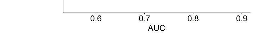
The capability of each feature to distinguish between the two classes is represented by the AUC
(Figure 5). For each of the seven groups, which were determined from the correlation matrix, the feature
with the highest AUC value was chosen and the remaining features were discarded. For example, out
of logLambda, mu_TS, and logN0, only logLambda was chosen in the final list of features.
The final selection of features, ordered by the AUC values, comprised of sd_Nt_10, sd_D0_10,
sd_log10_R_10, R, Z, D0_Nt, and logLambda. The correlation matrix and AUC values of the selected
features are provided in Figure 6.Atmosphere 2019, 10, 251 10 of 18
Atmosphere 2019, 10, x FOR PEER REVIEW 11 of 19
Figure 4. Correlation matrix of the rain microstructure parameters. Blank cells represent insignificant
Figure
Atmosphere 4. 10,
2019, Correlation matrix
x FOR PEER of the rain microstructure parameters. Blank cells represent insignificant
REVIEW 12 of 19
correlation with confidence level of 0.95.
correlation with confidence level of 0.95.
The capability of each feature to distinguish between the two classes is represented by the AUC
(Figure 5). For each of the seven groups, which were determined from the correlation matrix, the
feature with the highest AUC value was chosen and the remaining features were discarded. For
example, out of logLambda, mu_TS, and logN0, only logLambda was chosen in the final list of
features.
Figure 5. Relative
Figure importance
5. Relative importanceofofthe
therain
rainmicrostructure parametersexpressed
microstructure parameters expressed
by by
thethe
areaarea under
under the the
receiver operating characteristic curve (AUC) [67].
receiver operating characteristic curve (AUC) [67].
The final selection of features, ordered by the AUC values, comprised of sd_Nt_10, sd_D0_10,
sd_log10_R_10, R, Z, D0_Nt, and logLambda. The correlation matrix and AUC values of the selected
features are provided in Figure 6.Figure 5. Relative importance of the rain microstructure parameters expressed by the area under the
receiver operating characteristic curve (AUC) [67].
The final selection of features, ordered by the AUC values, comprised of sd_Nt_10, sd_D0_10,
sd_log10_R_10, R, Z, D0_Nt, and logLambda. The correlation matrix and AUC values of the selected
Atmosphere 2019, 10, 251 11 of 18
features are provided in Figure 6.
(a) (b)
Figure 6. (a) Correlation matrix where blank cells represent insignificant correlation with confidence
level of 0.95. (b) AUC values of the final list of selected features.
3.3. Performance
3.3. Performance of
of the
the ML
ML Methods
Methods
After applying
After applyingthe
thefive
fivedifferent
differentmachine-learning
machine‐learningclassification methods
classification on the
methods on FUR dataset,
the FUR their
dataset,
performances were measured by means of cross validation. High accuracy values were achieved
their performances were measured by means of cross validation. High accuracy values were achieved in
all cases, while the F-measure and Kappa were near 0.8 in the best cases (Figure 7). Four appeared
to be the optimum number of features to be used because the improvement beyond four parameters
was marginal. The RF models performed the best in most cases, followed by KNN, NB, and Ctree.
NB performed worse when the number of features exceeded four parameters. LDA performed the
worst. The performance of the NB method when using the four parameters (Z, Nt_4R, sd_log10(Nt)_30,
and sd_log10(R)_30) suggested in the Bu_15 method [11] (the red point in Figure 7) was lower than its
performance when using the four optimal parameters identified by the correlation matrix and AUC
(see Section 3.2).
When using the data from FUR to train the models and then testing them on the REG dataset,
the patterns of the performance indicators (Figure 8) were similar to the cross validation on the FUR
dataset (Figure 7); RF was still the best model, and four was again the optimum number of features.
Using RF with four parameters resulted in an accuracy of 98% and an F-measure and Kappa of 80%.
The NB performance dropped noticeably when using six parameters. It also dropped when using
the four parameters suggested in the Bu_15 method [11] (the red point in Figure 8). Remarkably,
Ctree achieved high performance indicators using only two parameters and its performance dropped
when using more than two parameters.was marginal. The RF models performed the best in most cases, followed by KNN, NB, and Ctree.
NB performed worse when the number of features exceeded four parameters. LDA performed the
worst. The performance of the NB method when using the four parameters (Z, Nt_4R,
sd_log10(Nt)_30, and sd_log10(R)_30) suggested in the Bu_15 method [11] (the red point in Figure 7)
was lower than its performance when using the four optimal parameters identified by the correlation
Atmosphere 2019, 10, 251 12 of 18
matrix and AUC (see Section 3.2).
Figure 7. Performance of the machine-learning classification methods with different numbers of
Figure 7. Performance of the machine‐learning classification methods with different numbers of
features. Each point is produced by taking the mean value of 200 repetitions of stratified cross validation
features. Each point is produced by taking the mean value of 200 repetitions of stratified cross
performed on the Fürstenzell dataset. The red point represents the performance of the Bu_15 method
validation performed on the Fürstenzell dataset. The red point represents the performance of the
with four parameters.
Bu_15 method with four parameters.
When using the data from FUR to train the models and then testing them on the REG dataset,
the patterns of the performance indicators (Figure 8) were similar to the cross validation on the FUR
dataset (Figure 7); RF was still the best model, and four was again the optimum number of features.
Using RF with four parameters resulted in an accuracy of 98% and an F‐measure and Kappa of 80%.
The NB performance dropped noticeably when using six parameters. It also dropped when using the
four parameters suggested in the Bu_15 method [11] (the red point in Figure 8). Remarkably, CtreeAtmosphere 2019, 10, x FOR PEER REVIEW 14 of 19
achieved high10,
Atmosphere 2019, performance
251 indicators using only two parameters and its performance dropped 13
when
of 18
using more than two parameters.
Figure 8. Performance of the machine-learning classification methods with different numbers of
Figure 8. Performance of the machine‐learning classification methods with different numbers of
features. Each model was trained on the Fürstenzell dataset and tested on the Regensburg dataset.
features. Each model was trained on the Fürstenzell dataset and tested on the Regensburg dataset.
The red point represents the performance of the Bu_15 method with four parameters.
The red point represents the performance of the Bu_15 method with four parameters.
4. Discussion
4. Discussion
The low percentage of convective rain intervals in the reference dataset (8.5%) explains the high
accuracylow
The percentage
of most methods of in
convective rain intervals
the literature in the reference
simply because dataset
they classify most (8.5%) explains
intervals the high
as stratiform
accuracy of most methods in the literature simply because they classify most intervals
rain. The F-measure and Kappa revealed clear differences in the performances of the different methods. as stratiform
rain. The F‐measure
The You_16, Ca_06, andandCa_08
Kappa revealed
methods clear
have highdifferences
accuracies.inHowever,
the performances
the Kappaofand theF-measure
different
methods.
values forThe You_16,
You_16 Ca_06,
are much and Ca_08
better methods
than those of thehave
otherhigh accuracies. However, the Kappa and F‐
methods.
measure values for You_16 are much better than those
The performance of You_16 compared to Br_09 provides clear of the otherevidence
methods. that adjusting the decision
The performance
boundary can considerablyof You_16
improvecompared to Br_09This
the performance. provides clear evidence
was confirmed again bythatthe adjusting
improvement the
decision boundary can considerably improve the performance.
achieved when optimizing the decision boundary by using LDA in three other cases.This was confirmed again by the
improvement achieved when optimizing the decision boundary by using LDA in
The performance of the modified Br_09 and You_16 methods indicates that using the combination three other cases.
of D0 andperformance
The log10 (Nw) toofclassify
the modified
rain typeBr_09 and You_16
is superior methods
to any other indicatessuggested
combination that using in the
the
combination of D0 and log 10(Nw) to classify rain type is superior to any other combination suggested
literature. This is in agreement with the findings of Thurai et al. [24] and explains the good performance
in the literature.
reported in variousThis is in agreement
papers despite thewith the findings
different of Thurai
geographical et al.and
locations [24]use
andofexplains
differentthe good
devices.
performance
However, after reported
adjustingin the
various papers
decision despiteTS_a
boundary, the and
different geographical
TS_b revealed very locations and for
similar values usethe
ofAtmosphere 2019, 10, 251 14 of 18
three performance indicators, i.e., accuracy, F-measure, and Kappa. This strongly suggests that the
parameters used in TS_a, TS_b, and Br_09 carry a sensitive signal that can successfully be used in
classifying the rain type.
As pointed out by Bukovčić et al. [11], two parameters are not sufficient to clearly separate
convective and stratiform rain. Many parameters have been suggested in the literature as potential
classifiers for the rain type. Our results show that many of these parameters are intercorrelated;
however, it is possible to limit the number of parameters to four while achieving a high performance.
The choice of these parameters is affected by the training dataset, the disdrometer type, and the prior
classification method. For example, Niu et al. [2] proposed using the spread of the measured velocities
across the diameter sizes. Our results suggest that this spread is correlated with Z, which is a better
classifier for the rain type. In addition, choosing the same parameters as Bukovčić et al. [11] resulted
in lower performance indicators than using the same method (NB) with the four best parameters,
as explained in Section 3.2. sd_R is also a very important parameter that can be used as a classifier.
However, it was not included in the feature selection process because it was already used in the
process of constructing the prior classification. In other cases (e.g., where the prior classification is
done by other methods such as using a wind profiler, radar, or satellite data), sd_R should also be
tested as a strong candidate among the classification parameters. We expect that other combinations
of parameters will be able to achieve even higher performance depending on the location, device
type, or the method of building the prior classification. However, we expect the improvement to be
marginal. The features presenting the fluctuation of the rain microstructure parameters generally have
the highest classification power, while fitted gamma distribution parameters have the lowest despite
being used widely in the literature [25–28,30].
The rain type classification was considerably improved by the ML classification models. Using the
seven most important features in the models revealed that RF performed the best in almost all cases,
closely followed by KNN and Ctree, while LDA had the lowest performance. This means that achieving
a better classification might also be possible by choosing different and more advanced predictive
models with different combinations of rain microstructure parameters.
For most of the tested models, the performance stabilizes when using four parameters.
The exceptions are LDA and NB. For LDA, five appears to be the critical number of parameters, which
is obvious in both the cross validation and the testing on the REG dataset. For NB, the performance
peaks and then drops again when further increasing the number of predictors. The likely reason for
this is that, in NB, it is assumed that the predictors are independent of each other even though the fifth
parameter Z has a high negative correlation with the fourth parameter R. In addition, note that this
drop in the performance might be influenced by the small size of the REG dataset. This small size
might also be the reason for the peak performance of Ctree with only two parameters when testing on
the REG dataset.
The ML models, which are trained on the FUR dataset and tested on the REG dataset, performed
well and with similar performance values when applying the cross validation. This indicates that it is
appropriate to train ML models for classifying the rain type in one location and use these models in
adjacent locations that have similar climate conditions. The spatial extent of the applicability of these
models however requires further investigation.
The initial choice of methods to construct the prior classification is definitely prone to errors and
inaccuracies. However, this choice was driven by the available data. Furthermore, observations of
cloud types are generally scarce, and this limited the size of our dataset. However, based on enhanced
prior classifications of cloud types, better classification models will be achievable. An improved
assessment of the performance of such models will need to include all rain intervals for a long time
period without discarding events with unclear or mixed cloud types. In the next step, we also suggest
classifying rain events into clearly defined convective, stratiform, and mixed events based on the
pattern of successive interval rain type classes produced by this method.Atmosphere 2019, 10, 251 15 of 18
5. Conclusions
Thies measurements of the rain microstructure were combined with cloud observations at two
sites in Bavaria in southern Germany to test the quality of rain type classification methods and suggest
improvements. A subset of the dataset was used to construct a reference classification and test the
classification models from the literature. Some machine-learning classification models were trained on
the data from FUR and then tested on the data from REG.
The simple dual parameter classification methods that had been built for other disdrometer types
performed poorly in their original form. However, the classification performance could be improved
via an objective specification of the decision boundary. The modified Br_09 [28] performed better than
the other methods.
The optimal features for classifying the rain type were those associated with the fluctuation of
the rain microstructure parameters over 10 min. Conversely, the parameters of the fitted gamma
distribution to the rain DSD were the least important.
Machine-learning rain type classification methods performed better than the simple dual parameter
classification methods when applied to Thies disdrometer measurements. RF methods performed the
best of the tested ML models, both via cross validation and when training the model in one location
and testing it in another. Four parameters are sufficient to reach high performance levels for the
classification model. The performance of the ML methods based on the rain microstructure features as
measured by other types of disdrometers needs to be investigated in the future.
We suggest using the same procedure of feature selection and model testing for future studies
after applying different methods for prior classification to build the training model, ideally using wind
profilers collocated with disdrometers of different types. The variation of the rain microstructure
in several locations in Bavaria will be investigated after classifying the rain type using this method.
We expect that this procedure of rain type classification will foster better quantitative estimations of
rain by remote sensors.
Author Contributions: Conceptualization, W.G. and A.M.; formal analysis, W.G.; supervision, A.M.;
writing—original draft, W.G.; writing—review and editing, W.G., N.E., and A.M.
Funding: This work was supported by the German Research Foundation (DFG) and the Technical University of
Munich (TUM) in the framework of the Open Access Publishing Program.
Acknowledgments: We thank the Deutscher Wetterdienst (German Meteorological Service DWD) for providing
Thies measurements and cloud observations. We also thank Anna-Maria Tilg for her valuable comments. The first
author thanks the Deutscher Akademischer Austauschdienst (DAAD) for financial support. We appreciate the
valuable comments provided by two anonymous reviewers.
Conflicts of Interest: The authors declare no conflict of interest. The funders had no role in the design of the
study; in the collection, analyses, or interpretation of data; in the writing of the manuscript; or in the decision to
publish the results.
References
1. Steiner, M.; Smith, J.A. Convective versus stratiform rainfall: An ice-microphysical and kinematic conceptual
model. Atmos. Res. 1998, 47–48, 317–326. [CrossRef]
2. Niu, S.; Jia, X.; Sang, J.; Liu, X.; Lu, C.; Liu, Y. Distributions of raindrop sizes and fall velocities in a semiarid
plateau climate: Convective versus stratiform rains. J. Appl. Meteorol. Climatol. 2010, 49, 632–645. [CrossRef]
3. Islam, T.; Rico-Ramirez, M.A.; Thurai, M.; Han, D. Characteristics of raindrop spectra as normalized gamma
distribution from a Joss–Waldvogel disdrometer. Atmos. Res. 2012, 108, 57–73. [CrossRef]
4. World Meteorological Organization. International Meteorological Vocabulary, 2nd ed.; Secretariat of the World
Meteorological Organization: Geneva, Switzerland, 1992; ISBN 9789263021823.
5. Thompson, E.J.; Rutledge, S.A.; Dolan, B.; Thurai, M. Drop size distributions and radar observations of
convective and stratiform rain over the equatorial Indian and West Pacific Oceans. J. Atmos. Sci. 2015, 72,
4091–4125. [CrossRef]Atmosphere 2019, 10, 251 16 of 18
6. Houze, R.A. Stratiform precipitation in regions of convection: A meteorological paradox? Bull. Am.
Meteorol. Soc. 1997, 78, 2179–2196. [CrossRef]
7. Ferrier, B.S.; Tao, W.-K.; Simpson, J. A double-moment multiple-phase four-class bulk ice scheme. Part II:
Simulations of convective storms in different large-scale environments and comparisons with other bulk
parameterizations. J. Atmos. Sci. 1995, 52, 1001–1033. [CrossRef]
8. Ghada, W.; Buras, A.; Lüpke, M.; Schunk, C.; Menzel, A. Rain microstructure parameters vary with large-scale
weather conditions in Lausanne, Switzerland. Remote Sens. 2018, 10, 811. [CrossRef]
9. Bringi, V.N.; Chandrasekar, V.; Hubbert, J.; Gorgucci, E.; Randeu, W.L.; Schoenhuber, M. Raindrop size
distribution in different climatic regimes from disdrometer and dual-polarized radar analysis. J. Atmos. Sci.
2003, 60, 354–365. [CrossRef]
10. Llasat, M.-C. An objective classification of rainfall events on the basis of their convective features: Application
to rainfall intensity in the northeast of Spain. Int. J. Climatol. 2001, 21, 1385–1400. [CrossRef]
11. Bukovčić, P.; Zrnić, D.; Zhang, G. Convective–stratiform separation using video disdrometer observations in
central Oklahoma—The Bayesian approach. Atmos. Res. 2015, 155, 176–191. [CrossRef]
12. Berg, P.; Moseley, C.; Haerter, J.O. Strong increase in convective precipitation in response to higher
temperatures. Nat. Geosci. 2013, 6, 181–185. [CrossRef]
13. Langer, I.; Reimer, E. Separation of convective and stratiform precipitation for a precipitation analysis of the
local model of the German weather service. Adv. Geosci. 2007, 10, 159–165. [CrossRef]
14. Houze, R.A. Cloud Dynamics, 2nd ed.; Elsevier: Amsterdam, NY, USA, 2014; ISBN 978-0-12-374266-7.
15. Rulfová, Z.; Kyselý, J. Disaggregating convective and stratiform precipitation from station weather data.
Atmos. Res. 2013, 134, 100–115. [CrossRef]
16. Williams, C.R.; Ecklund, W.L.; Gage, K.S. Classification of precipitating clouds in the tropics using 915-MHz
wind profilers. J. Atmos. Ocean. Technol. 1995, 12, 996–1012. [CrossRef]
17. Steiner, M.; Houze, R.A.; Yuter, S.E. Climatological characterization of three-dimensional storm structure
from operational radar and rain gauge data. J. Appl. Meteorol. 1995, 34, 1978–2007. [CrossRef]
18. Churchill, D.D.; Houze, R.A. Development and structure of winter monsoon cloud clusters on 10 December
1978. J. Atmos. Sci. 1984, 41, 933–960. [CrossRef]
19. Kummerow, C.; Hakkarinen, I.M.; Pierce, H.F.; Weinman, J.A. Determination of precipitation profiles from
airborne passive microwave radiometric measurements. J. Atmos. Ocean. Technol. 1991, 8, 148–158. [CrossRef]
20. Berendes, T.A.; Mecikalski, J.R.; MacKenzie, W.M.; Bedka, K.M.; Nair, U.S. Convective cloud identification
and classification in daytime satellite imagery using standard deviation limited adaptive clustering.
J. Geophys. Res. 2008, 113, 909. [CrossRef]
21. Anagnostou, E.N.; Kummerow, C. Stratiform and Convective Classification of rainfall using SSM/I 85-GHz
brightness temperature observations. J. Atmos. Ocean. Technol. 1997, 14, 570–575. [CrossRef]
22. Adler, R.F.; Negri, A.J. A satellite infrared technique to estimate tropical convective and stratiform rainfall.
J. Appl. Meteorol. 1988, 27, 30–51. [CrossRef]
23. Yuter, S.E.; Houze, R.A. Measurements of raindrop size distributions over the pacific warm pool and
implications for Z–R relations. J. Appl. Meteorol. 1997, 36, 847–867. [CrossRef]
24. Thurai, M.; Gatlin, P.N.; Bringi, V.N. Separating stratiform and convective rain types based on the drop size
distribution characteristics using 2D video disdrometer data. Atmos. Res. 2016, 169, 416–423. [CrossRef]
25. Tokay, A.; Short, D.A. Evidence from tropical raindrop spectra of the origin of rain from stratiform versus
convective clouds. J. Appl. Meteorol. 1996, 35, 355–371. [CrossRef]
26. Caracciolo, C.; Prodi, F.; Battaglia, A.; Porcu, F. Analysis of the moments and parameters of a gamma DSD
to infer precipitation properties: A convective stratiform discrimination algorithm. Atmos. Res. 2006, 80,
165–186. [CrossRef]
27. Caracciolo, C.; Porcù, F.; Prodi, F. Precipitation classification at mid-latitudes in terms of drop size distribution
parameters. Adv. Geosci. 2008, 16, 11–17. [CrossRef]
28. Bringi, V.N.; Williams, C.R.; Thurai, M.; May, P.T. Using dual-polarized radar and dual-frequency profiler for
DSD characterization: A case study from Darwin, Australia. J. Atmos. Ocean. Technol. 2009, 26, 2107–2122.
[CrossRef]
29. Uijlenhoet, R.; Steiner, M.; Smith, J.A. Variability of raindrop size distributions in a squall line and implications
for radar rainfall estimation. J. Hydrometeorol. 2003, 4, 43–61. [CrossRef]You can also read