Map Matching for Semi-Restricted Trajectories - DROPS
←
→
Page content transcription
If your browser does not render page correctly, please read the page content below
Map Matching for Semi-Restricted Trajectories
Timon Behr        #
University of Konstanz, Germany
Thomas C. van Dijk          #
University of Bochum, Germany
Axel Forsch      #
University of Bonn, Germany
Jan-Henrik Haunert               #
University of Bonn, Germany
Sabine Storandt         #
University of Konstanz, Germany

      Abstract
We consider the problem of matching trajectories to a road map, giving particular consideration
to trajectories that do not exclusively follow the underlying network. Such trajectories arise, for
example, when a person walks through the inner part of a city, crossing market squares or parking
lots. We call such trajectories semi-restricted. Sensible map matching of semi-restricted trajectories
requires the ability to differentiate between restricted and unrestricted movement. We develop in this
paper an approach that efficiently and reliably computes concise representations of such trajectories
that maintain their semantic characteristics. Our approach utilizes OpenStreetMap data to not only
extract the network but also areas that allow for free movement (as e.g. parks) as well as obstacles
(as e.g. buildings). We discuss in detail how to incorporate this information in the map matching
process, and demonstrate the applicability of our method in an experimental evaluation on real
pedestrian and bicycle trajectories.
2012 ACM Subject Classification Information systems → Geographic information systems
Keywords and phrases map matching, OpenStreetMap, GPS, trajectory, road network
Digital Object Identifier 10.4230/LIPIcs.GIScience.2021.II.12
Supplementary Material Software: https://github.com/tcvdijk/tessa
   archived at swh:1:dir:265a254805a64ab73036cdebd99b59590052a471
Funding Timon Behr: DFG Grant Sto 1114/4-2 in Priority Programme 1894 “Volunteered Geo-
graphic Information”.
Thomas C. van Dijk: DFG Grant Di 2161/2-2 in Priority Programme 1894 “Volunteered Geographic
Information”.
Axel Forsch: DFG Grant Ha 5451/7-1 in Priority Programme 1894 “Volunteered Geographic
Information”.

 1      Introduction
Map matching is the process of pinpointing a trajectory (given e.g. as a sequence of GPS
measurements) to a path in an underlying network. The goal is to find the path that explains
the observed measurements best. Map matching is often the first step of trajectory data
processing as there are several benefits when dealing with paths in a known network instead
of raw location measurement data:
    Both location measurements and geometric representations of roads are usually imprecise.
    Hence, constraining the trajectory to a path in a network is necessary to integrate the
    information given with a trajectory (e.g. recorded speed, vehicle type) with information
    given with the road data (e.g. speed limit, road type). This is important to enable
    applications as movement analysis or real-time navigation [17, 28].
            © Timon Behr, Thomas C. van Dijk, Axel Forsch, Jan-Henrik Haunert, and Sabine Storandt;
            licensed under Creative Commons License CC-BY 4.0
11th International Conference on Geographic Information Science (GIScience 2021) – Part II.
Editors: Krzysztof Janowicz and Judith A. Verstegen; Article No. 12; pp. 12:1–12:16
                   Leibniz International Proceedings in Informatics
                   Schloss Dagstuhl – Leibniz-Zentrum für Informatik, Dagstuhl Publishing, Germany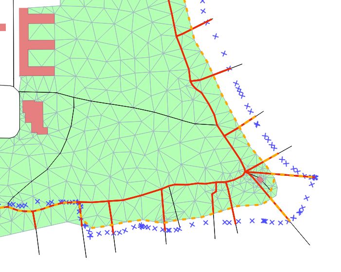
12:2   Map Matching for Semi-Restricted Trajectories

           Storing raw data is memory-intensive (especially with high sampling densities). Paths in a
           given network on the other hand can be stored very compactly and many indexing methods
           have been developed that allow huge path sets to be queried efficiently [10, 15, 25].
           Matching a trajectory to the road network enables data mining techniques that link
           attributes of the road network to attributes of the trajectories. This is used to deduce
           routing preferences from given trajectories [27, 19, 9, 4]. To analyze and compare multiple
           trajectories, the trajectories need to be matched to a common network beforehand.
       However, if the assumption that a given trajectory was derived from restricted movement in a
       certain network is incorrect, map matching might heavily distort the trajectory and possibly
       erase important semantic characteristics. For example, there could be two trajectories of
       pedestrians who met in the middle of a market square, arriving from different directions.
       After map matching, not only the aspect that the two trajectories got very close at one point
       would be lost but the visit of the market square would be removed completely (if there are
       no paths across it in the given network). Not applying map matching at all might result in
       misleading results as well, though, as the parts of the movement that actually happened in a
       restricted fashion might not be discovered and – as outlined above – having to store and
       query huge sets of raw trajectories is undesirable.
           Hence, the goal of this paper is to design an approach that allows for sensible map
       matching of trajectories that possibly contain on- and off-road sections, which we call semi-
       restricted trajectories. We will show that our approach computes paths that are significantly
       more compact than the raw trajectory data but at the same time still faithfully represent
       the original movement.

       1.1    Related work
       Due to its practical relevance, there is a huge body of work on map matching. As we cannot
       cover all the respective papers here in detail, we will focus on related work most relevant to
       our envisioned application scenario.

       Map matching for restricted trajectories. According to a recent survey on map matching
       [6], existing algorithms can be classified into four categories based on the underlying matching
       principle: similarity models, state-transition models, candidate-evolving models and scoring
       models. We will now mainly discuss state-transition models as our approach will fit in this
       category. Early approaches for map matching relied on purely geometric similarities between
       the road network and the recorded trajectories [31]. One problem of these approaches is their
       sensitivity to measurement noise and low sampling rates. In order to overcome this problem,
       more sophisticated approaches try to model sensible transitions between consecutive states.
       In this context, e.g. Hidden Markov Models (HMM) [11, 14, 18] and reinforcement learning
       techniques [20, 33] were applied successfully. Furthermore, the incorporation of guiding
       assumptions, e.g. that movements most likely follow shortest paths, can help to compute
       more meaningful matches and also to decrease the running time [7, 13].

       Off-road and free space map matching. Map matching might also lead to artifacts in
       case the movement did indeed happen in an underlying network but the network data is
       incomplete. Hence, several approaches have been developed that still produce high-quality
       matches in this scenario by allowing the path to contain off-road sections [1, 11, 23]. However,
       these approaches rely on the assumption that the unrestricted movement sequences are rather
       short which does not have to be the case when dealing with semi-restricted trajectories. Map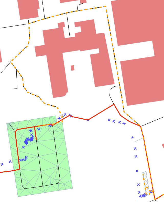
T. Behr, T. C. van Dijk, A. Forsch, J.-H. Haunert, and S. Storandt 12:3
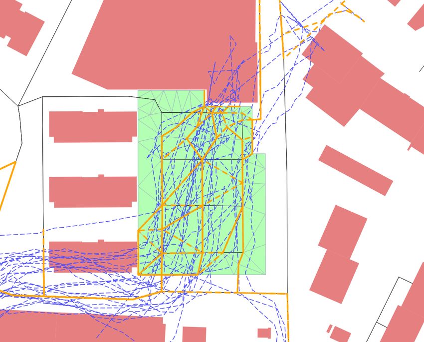
Figure 1 Example of a map with an embedded road network as well as free spaces and obstacles.
The blue measurement-based trajectory is best explained by movement along the orange dashed
path, which follows roads and free spaces where possible but contains no obstacle intersections.
matching for outdoor pedestrian trajectories with a high degree of freedom often requires
additional data to yield good results as e.g. derived from a smartphone accelerometer or
compass [22, 24]. In other lines of work, the goal is to model the possible movement network as
precise as possible (including e.g. cross walks) to be able to adapt conventional map matching
techniques for restricted movement [2]. Most map matching approaches for pedestrians
focus on indoor movement, though [26, 32, 34]. But these approaches do not consider the
possibility to switch between restricted and unrestricted movement and also do not scale
well enough to deal with large networks and rich map context.
Representation methods for unrestricted trajectories. Existing methods for storing and
indexing raw trajectories are often based on a partitioning of the ambient space e.g. into
equisized grid cells or by constructing spatial data structures as CSE-Trees [29], ST-R-trees or
TB-trees [21]. But these approaches do not feature any kind of compression and are slow in
case large trajectory sets are to be reported in a query. In contrast, map-matched trajectories
can be managed much more efficiently in terms of memory and retrieval time using methods
as SPNET [15], PRESS [25] or PATHFINDER [10]. To gain these advantages also when
dealing with unrestricted trajectories, methods for computing an underlying graph for a given
set of trajectories were investigated [5]. This task is closely related to map generation from
trajectory sets [12, 16]. However, these methods either discard outlier trajectories completely
or produce rather large graphs, which is both undesirable in our application. Furthermore,
the computed graphs have to be updated whenever new trajectories arrive. We will discuss
methods to produce graphs that cover free space areas in such a way that all trajectories
that may traverse said free space are represented sufficiently well. This problem has also
been investigated in the context of indoor navigation. One approach is to represent the
traversable space of floor plans by their skeleton, incorporating points of interest such as
entrances and exits [8].
1.2 Contribution
We present a pipeline that can accurately map match semi-restricted trajectories, thereby
overcoming several limitations of previous work. We consider the following points to be our
main contribution:
GIScience 202112:4 Map Matching for Semi-Restricted Trajectories
We propose an extended network model capable of handling semi-restricted trajectories.
In addition to the general graph representation of linear streets, we add tessellated
free-space polygons that represent areas of unrestricted movement (such as marketplaces
or parking lots). We discuss how a sensible tessellation can be obtained and provide an
open source implementation at https://github.com/tcvdijk/tessa.
We significantly extend the map matching approach presented in [11], which was originally
developed to enable map matching on incomplete road network data. First, we make
the approach more efficient by incorporating ideas from [7]. More importantly, though,
we make the algorithm work on our extended network model. Among other things, this
requires a carefully designed penalization scheme for off-road sections.
Furthermore, we describe how to incorporate obstacles in the tessellation as well as the
map matching process. Obstacles are polygons that the map matched path is not allowed
to intersect (as e.g. buildings for cycle trajectories). Taking obstacles into account requires
additional processing steps but allows us to produce more meaningful results.
We evaluate our approach in an extensive experimental study on real trajectories. We
investigate the accuracy of the computed paths, in particular with respect to the recogni-
tion of unrestricted movement sections. Figure 1 shows an example outcome of our map
matching pipeline.
2 Methodology
In this section we develop our map-matching algorithm for semi-restricted trajectories, starting
with a baseline method for trajectories restricted to a network (Section 2.1) and extending it
to deal with outliers, missing segments in the road data, and matches on designated free
spaces (Section 2.2).
2.1 A baseline algorithm for trajectories restricted to a network
Our algorithm is based on a state-transition model where each point of a given trajectory is
represented by a set of matching candidates – the possible system states, i.e., positions of a
moving subject. This is similar to HMM-based map-matching algorithms, which aim to find
a sequence of positions maximizing a product of probabilities, each of which corresponds to
a system state or a state transition. In contrast, we aim to minimize a sum of energy terms.
By introducing weights for the energy terms that can be controlled with interactive sliders,
the user of the algorithm has an intuitive tool for finding a good parameter setting.
Input requirements. The algorithm works on a trajectory T = ⟨p1 , . . . , pk ⟩ of k points in
R2 , which we will call the GPS-points. Additionally, we have a directed, edge-weighted graph
G = (V, E) that models the transport network. Every directed edge uv ∈ E corresponds to
a directed straight-line segment representing a road segment with an allowed direction of
travel. For a road segment that can be traversed in both directions, E contains the directed
edges uv and vu. For an edge e, let w(e) be its weight. In the basic setting, we will use the
Euclidean length as the weight, but note that other values are possible.
System states. For every GPS-point pi , we compute a set of matching candidates by
considering a disk Di of prescribed radius r around pi : we select all road segments intersected
by Di and pick the point nearest to pi on each. If such a point is not a node of G, we
inject it as a new node v. (This means that we split each directed edge uw containing vT. Behr, T. C. van Dijk, A. Forsch, J.-H. Haunert, and S. Storandt 12:5
into two directed edges uv and vw; we distribute the weight of uw to the edges uv and vw
proportionally to their lengths.) As a consequence, the set of matching candidates for pi is a
set of nodes Vi ⊆ V . If Vi is empty, we discard the GPS-point pi and do not consider it for
the matching.
State transitions. Possible transitions between candidates for two consecutive GPS-points
are not modelled explicitly. Instead, they are implicitly modeled with the graph G by
assuming that the transition between any two matching candidates u ∈ Vi and v ∈ Vi+1
occurs via a minimum-weight u-v-path in G. Accordingly, the matched output path P is
defined by selecting, for i = 1, . . . , k, one candidate vi from the set Vi and connecting every
pair of consecutive nodes in the sequence ⟨v1 , . . . , vk ⟩ via a minimum-weight path.
Energy model. To ensure that the output path P matches well to the trajectory, we set
up and minimize an energy function that aggregates a state-based and a transition-based
energy:
Pk 2
The state-based energy is i=1 ∥pi − vi ∥ , meaning that the energy increases quadratically
with the Euclidean distance between a GPS-point pi and the matching candidate vi
selected for it.
Pk−1
The transition-based energy is i=1 w(Pi,i+1 ), where Pa,b is a minimum-weight va -vb -
path in G and w(P ) is the total weight of a path P (i.e., the sum of the weights of the
edges of P ). For now, we use the geometric length of an edge as its weight.
The two energies are aggregated using a weighted sum, parametrized with a parameter αc .
This yields our overall objective function quantifying the fit between a trajectory ⟨p1 , ..., pk ⟩
and an output path defined with the selected sequence ⟨v1 , ..., vk ⟩ of nodes:
k
X k−1
X
2
Minimize E(⟨p1 , ..., pk ⟩, ⟨v1 , ..., vk ⟩) = αc · ∥pi − vi ∥ + w(Pi,i+1 ) (1)
i=1 i=1
Algorithm. An optimal solution is computed using k runs of Dijkstra’s algorithm on a graph
that results from augmenting G with a few auxiliary nodes and arcs. More precisely, we use
an incremental algorithm that proceeds in k iterations. In the i-th iteration, it computes for
the sub-trajectory ⟨p1 , . . . , pi ⟩ of T and each matching candidate v ∈ Vi the objective value
Eiv of a solution ⟨v1 , ..., vi ⟩ that minimizes E(⟨p1 , . . . , pi ⟩, ⟨v1 , . . . , vi ⟩) under the restriction
that vi = v. This computation is done as follows.
For i = 1 and any node v ∈ V1 , E1v is simply the state-based energy for v, i.e., E1v =
2
αc · ∥p1 − v∥ .
For i > 1, we introduce a dummy node si and a directed edge si u for each u ∈ Vi−1
u
whose weight we set as Ei−1 ; see Fig. 2. With this, for any node v ∈ Vi , Eiv corresponds to
the weight of a minimum-weight si -v-path in the augmented graph, plus the state-based
energy for v. We are thus interested in finding for si and every node in Vi a minimum-
weight path. All these paths can be found with one single-source shortest path query
with source si and, thus, with a single execution of Dijkstra’s algorithm.
We observe that our objective function E(⟨p1 , . . . , pi ⟩, ⟨v1 , . . . , vi ⟩) for the whole trajectory
has the minimum value minv∈Vk {Ekv } and is among the values we have computed. It is not
difficult to maintain information during the run of the algorithm to enable the reconstruction
of a solution attaining that value.
GIScience 202112:6 Map Matching for Semi-Restricted Trajectories
u
v
Vi−1
pi−1
pi
w
si
Vi
Figure 2 The incremental step of our algorithm. From the dummy node si , shortest paths to all
nodes in Vi are computed with one single-source shortest path query (see the dashed lines). The
weight of each such path plus the state-based energy of the corresponding terminal is used as the
weight of a dummy edge in the next iteration.
p4 p4
p2 p3 p2 p3
p5 p5
p1 p1
(a) (b)
Figure 3 (a) Forcing the input trajectory (blue points) to the road network can cause a long
detour in the output path (dashed). (b) Additional unmatched candidates and connecting segments
prevent the detour.
2.2 Extensions for semi-restricted trajectories
The algorithm outlined in the previous section forces the output path to the road network,
which can lead to unfavorable solutions. Consider the example in Figure 3, where road
segments are missing in the road data. By forcing the output path to the road network, a
long and unrealistic detour is generated. More generally, we deal with the following issues:
The trajectory contains outliers.
The road data is incomplete, i.e., road segments are not modeled in the data.
The trajectory traverses open spaces that are modeled as areas.
To deal with the first two issues, we allow GPS-points to be left unmatched and accordingly
introduce unmatched candidates. The third issue is handled by augmenting the road network
with additional edges, which we call off-road segments. Accordingly, a matching candidate on
an off-road segment is called off-road candidate. We present these concepts in the following
in detail and then describe how we extend the energy model.
Unmatched candidates. For each GPS-point pi we extend the set of candidates with a
candidate at the observed location. Analogously to the baseline algorithm, we add this
candidate into the graph by inserting it as a node ui . For every node vi−1 in the candidate
set of GPS-point pi−1 and every node vi+1 in the candidate set of GPS-point pi+1 we addT. Behr, T. C. van Dijk, A. Forsch, J.-H. Haunert, and S. Storandt 12:7
Vi−1
pi−1
pi
si
Vi
Figure 4 Extended graph to support unmatched segments. In addition to the candidates in the
road network, every GPS-point is treated as a candidate itself. Additional arcs (green) are introduced
connecting unmatched candidates (blue) to all candidates of the previous and next GPS-point.
directed edges vi−1 ui and ui vi+1 , respectively. Figure 4 shows the extended graph for two
consecutive GPS-points with the additional edges shown in green. This approach guarantees
that there is always a fallback solution, which can be chosen if no path in the road network is
similar to the trajectory. We will associate the additional edges with high energy (see below)
to ensure that they will be chosen only if necessary. In the following we refer to the baseline
method with the extension to unmatched candidates as Baseline+.
Off-road candidates. Open spaces such as public squares, parks or parking lots are repres-
ented as polygonal areas in most data sources. The algorithm as described so far does not
deal with this (see Figure 5a). We extend the road network by triangulating all open spaces
and adding tessellation edges as arcs into the graph (Figure 5b). In order to accurately
represent polygons of varying degrees of detail and to provide an appropriate number of
off-road candidates, we use CGAL’s meshing algorithm [3] with an upperbound on the length
of the resulting edges and a lowerbound on the angles inside triangles. As seen in the figure,
this algorithm can introduce additional nodes to achieve these constraints. Note that original
road segments can cross open spaces: this should be respected by the tessellation since we
will give preference to on-road candidates over off-road candidates.
Extensions of energy model. With the addition of the extensions to the baseline algorithm
we now have three different sets of edges in the graph: the original edges of the road network
Er , the edges incident to unmatched candidate nodes Eu and the off-road edges on open
spaces Et . We prefer on-road matches over off-road matches while unmatched candidates are
used as a fallback solution and thus should only be selected if no suitable path over on- and
off-road edges can be found. To model this we adapt the energy function by changing the
edge weighting w of the graph. We introduce two weighting terms αt and αu that scale the
weight w(e) of each edge e in Et or Eu , respectively. The edge weighting function thus is
defined as:
ℓ(e), e ∈ Er
w(e) = αu · ℓ(e), e ∈ Eu (2)
α · ℓ(e), e ∈ E
t t
To favor matches in the original road network and keep unmatched candidates as a fallback
solution, 1 < αt < αu should hold. Together with the weighting factor αc for the state-based
energy our final energy function thus comprises three different weighting factors.
GIScience 202112:8 Map Matching for Semi-Restricted Trajectories
(a) (b)
Figure 5 (a) Roads in the network data. Movement on the open space (green) cannot be matched
appropriately (dashed). (b) Extended road network. Open spaces are tessellated in order to add
appropriate off-road candidates. Note that the green polygon has a hole, which remains untessellated
since it is not actually open space. Also note that additional vertices are added to prevent skinny
triangles.
3 Experiments
In this section, we evaluate the presented algorithm on real-world data. For this we conduct
a user study in the area of Constance, Germany. In Section 3.1, we describe the used data
sources and our experimental setup. In Section 3.2, we present a detailed analysis of the
quality of the produced map matching results.
3.1 Experimental setup
In our experiments we used data extracted from OpenStreetMap1 (OSM) to model the road
network. As input trajectories we use trajectories of pedestrians and cyclists recorded within
the scope of a user study. In the following we will explain this setup in detail.
Modelling the road network. Our experimental region is composed of the area around
Lake Constance, Germany. For this region we extract data from OSM to build the model of
the road network we use for matching. Elements tagged as highway are used to generate
the road network as described in Section 2.1. To make the road network feasible for cyclists
and pedestrians we removed all roads that are not traversable for these modes of transport.
Altogether we extracted a road graph with 931,698 nodes and 2,013,590 directed edges.
The open spaces used for tessellation are identified by extracting polygons with special
tags. We handpicked a list of tags representing spaces with unrestricted movement and tags
representing obstacles for movement. As the polygons we extracted this way overlapped in
some areas we had to sanitize the input: in the case that an obstacle overlapped an open
space we cropped the open space to not be covered by the obstacle. In the case that two
open spaces overlapped we split the open spaces such that no overlap exists in the final data.
This way we extracted 6827 polygons representing open spaces.
1
© OpenStreetMap contributorsT. Behr, T. C. van Dijk, A. Forsch, J.-H. Haunert, and S. Storandt 12:9
For the tessellation of the open spaces we decided on an upper bound of 25 meters for the
length of the resulting edges and kept the lower bound for the inside angles of the triangles at
the CGAL default value of about 20.6◦ . We decided on these parameters by visual inspection
of tessellation results. Together with the additional edges of the tessellation our final graph
consists of 1,148,213 nodes and 3,345,426 directed edges.
User study. To evaluate the performance of the algorithm we conducted a user study with
five paricipants. The participants were asked to record their trips while cycling or walking
with their mobile phones or similar GPS-devices. After each trip, the participant annotated
all sections of the trip where he or she left roads. This information serves as ground-truth
for our evaluation to determine weather these segments got identified correctly. In total, we
gathered 58 trajectories during the study. The length of these trajectories varies from 300
meters to 41.3 kilometers, and they contain 66 annotated off-road segments.
3.2 Map matching results
We evaluate our proposed map matching algorithm for semi-restricted trajctories in two
steps: In the first step, we investigate the sensitivity of our algorithm to parameter choices in
the energy model discussed in Section 2.1 and 2.2, and deduce a sensible parameter setting
thereupon. In the second step, we analyze our matching results more thoroughly and compare
them to the Baseline+ algorithm without tessellation.
Parameter tuning. There are three crucial parameters in our extended energy model that
govern the map matching process. First, we have the edge cost coefficients αt and αu ,
which for values larger than one penalize the usage of tessellation edges or edges incident
to unmatched points, respectively, in comparison to the usage of edges in the road network.
Furthermore, the parameter αc allows us to fine-tune the impact of the Euclidean distance
from a trajectory point to its matched point on the map in the objective function.
As we consider the inclusion of edges incident to unmatched points as a last resort, we
set αu to 10 in all our experiments. This value is sufficiently large to avoid unmatched points
whenever there are road network or tessellation edges in the proximity but it is also small
enough to not induce unreasonably long detours if the trajectory indeed crosses an area that
has no roads and is also not a free space according to our data set. For αt and αc the best
setting is less obvious, though. For too large αt and too small αc , the algorithm would match
trajectories only to paths in the road network. But a too large value αc would render the
algorithm too inflexible to find reasonable paths, especially in the presence of outliers.
We hence conducted the following experiment to see how sensitive our algorithm is to the
choice of αt and αc , and to figure out which configuration to use in subsequent studies: We
varied αt from 1.0 to 3.0 in increments of 0.1 and αc from 0.01 to 0.1 in increments of 0.01.
For the resulting 310 combinations, we assessed how well the algorithm identifies restricted
and unrestricted movement in our labeled trajectory benchmark set. More precisely, we
compared the true positive rate of correctly recognized off-road segments (the higher the
better) and the false positive rate of actual road parts treated as off-road segments (the lower
the better). The results are summarized in Figure 6, left. The effect of certain parameter
combinations for the matching of an off-road part is illustrated in Figure 6, right.
A significant range of value combinations is clearly dominated by others, in particular
the ones with αt > 2 or αc < 0.05. For αt close to 1.0, unsurprisingly, we have the highest
true positive rate; but also the highest false positive rate for αt in [1.0, 2.0]. For αc < 0.5 the
true positive rate is rather small. For αc chosen larger than that, we see that the precise
GIScience 202112:10 Map Matching for Semi-Restricted Trajectories
αt
0.7
1.0 2.1
1.1 2.2
1.2 2.3
1.3 2.4
1.4 2.5
0.6 1.5 2.6
1.6 2.7
1.7 2.8
1.8 2.9
true positive rate
1.9 3.0
2.0
0.5
αc
0.01
0.02
0.03
0.4 0.04
0.05
0.06
0.07
0.08
0.09
0.3
0.10
0.200 0.225 0.250 0.275 0.300
false positive rate
Figure 6 Left: Classification results for off-road section identification for different parameter
configurations. Right: Effect of the parameter choice illustrated for an example instance. In the
upper image (αt = 1.5, αc = 0.01), the GPS points (blue crosses) are matched to the cheap road
network edges whenever possible. In the middle image (αt = 1.5, αc = 0.10), the increased candidate
cost leads to a matching which deviates from the measurements as little as possible. In the lower
image (αt = 1.1, αc = 0.01), the decreased tessellation edge cost leads to more deviation from the
road network as in the upper image. Despite those differences, we observe that the middle part is
matched to the same edges for all three configurations.
choice is not that important as αt then seems to have a stronger influence on the achieved
trade-offs. Furthermore, we computed precision and recall for the identification of on-road
sections for all parameter combinations with the results that both, precision and recall, tend
to be close to 1.0 for all tested αt and αc . We hence conclude that the algorithm is not overly
sensitive to the precise parameter choice. For subsequent experiments we chose αt = 1.1 and
αc = 0.07.
Quality analysis. In the parameter tuning experiment, we just considered whether off- and
on-road sections were identified as such but now we want to further analyze the overall
matching quality, and compare our extended approach for semi-restricted map matching
to Baseline+ that does not use tessellated free spaces. We will focus on the following two
aspects in our comparative evaluation: (i) shape preservation of the input trajectories, (ii)
compression and indexing of trajectory sets.
To measure how well the shape of the original trajectory is preserved by our map matching
approach, we compute the Fréchet distance and the Dynamic Time Warping (DTW) distance
between the input and the output curve.T. Behr, T. C. van Dijk, A. Forsch, J.-H. Haunert, and S. Storandt 12:11
200 100
150 75
fréchet distance [m]
normalized dtw [m]
100 50
50 25
0
0
0 25 50 75 100 0 25 50 75 100
Figure 7 Fréchet and normed DTW distance between input trajectories and the matched paths
produced with our approach (blue) and Baseline+ (red). In both cases the trajectories (distributed
over the x-axis) are sorted by the fréchet distance (resp. normed DTW) of our approach.
▶ Definition 1 (Fréchet Distance). Given two polylines L, L′ with length k and k ′ , respectively,
the Fréchet distance is defined as dF (L, L′ ) := inf σ,θ maxt∈[0,1] ||L(σ(t)) − L′ (θ(t))||2 where
σ : [0, 1] → [1, k] and θ : [0, 1] → [1, k ′ ] are continuous and monotonic and σ(0) = θ(0) =
1, σ(1) = k and θ(1) = k ′ .
▶ Definition 2 (DTW Distance). Given two polylines L, L′ with length k and k ′ , respectively,
the DTW distance is the cost of a cheapest warping path between L and L′ . A warping path
′
is a sequence p = (p1 , . . . , pW ) with pw = (lw , lw ) ∈ [1 : k] × [1 : k ′ ] for w ∈ [1 : W ] such
′
that p1 = (1, 1) and pW = (k, k ), and pw+1 − pw ∈ {(1, 0), (0, 1), (1, 1)} for w ∈ [1 : W − 1].
PW
Thereby, the cost of path p is defined as i=1 ||pi ||2 . The normed DTW distance is the cost
of the path divided by 2 · max{k, k ′ }.
The Fréchet distance is a bottleneck measure that sometimes is even used as the main
objective for map matching [30]. DTW is frequently used in similarity analysis of time series
and other sequenced data, and has the advantage that its value is determined by the whole
shapes and not just by a local dissimilarity maximum. We always use the normed DTW
distance here, as it allows for better comparability between input trajectories of different
length. Figure 7 show the Fréchet and DTW distances for all off-road sections identified in
the user study; map matched by our algorithm as well as Baseline+. Although Baseline+ is
more likely to keep original trajectory points in the map matched path whenever free spaces
are traversed – and hence the shape therein should be perfectly preserved – we observe that
our tessellation based approach achieves comparable or even better shape similarity on most
inputs. On average, paths computed with our approach had a Fréchet/DTW distance to the
original trajectory of 31.81/16.25 while for Baseline+ the respective values are 32.52/18.47.
A possible reason for the better shape preservation with our approach is that transitions
between restricted and unrestricted movement tend to be smoother, see Figure 8 for an
example.
Next, we want to further evaluate whether the tessellation based addition of roughly
1.3 million edges to the road network is worthwhile not only for shape preservation and
unrestricted movement identification but also for compression purposes. To this end, we
GIScience 202112:12 Map Matching for Semi-Restricted Trajectories
Figure 8 Original GPS measurements (blue crosses) and matched paths produced by the
tessellation based approach (upper image) and Baseline+ (lower image). In the tessellation based
matching the shape of the original trajectory is faithfully preserved and the unrestricted movement
is correctly identified and matched to tessellation points and edges. Using Baseline+, the first part
of the unrestricted movement is wrongfully matched to the path network and subsequently the shape
is locally distorted when the switch from restricted to unrestricted movement occurs.T. Behr, T. C. van Dijk, A. Forsch, J.-H. Haunert, and S. Storandt 12:13
Figure 9 Upper left: Set of trajectories (dashed blue lines) traversing the same free space. The
yellow edges indicate their matched paths. Lower left: Trajectory (blue crosses) following the shore
line of the lake. The Baseline+ approach matches this trajectory to rather far apart paths as well as
several groynes, while the tessellation based approach produces a more sensible match. Right: In
the absence of sufficient tessellation edges, a trajectory traversing a large free space might end up
being matched to a path with a rather large detour.
count holes in the matched paths. Here, a hole is a continuous subpath that is not represented
by edges in the created graph but uses edges incident to unmatched points. The usage of
Baseline+ led to 43% more holes than the tessellation based approach. Furthermore, the
holes resulting from Baseline+ are typically significantly longer. Holes require additional
storage and indexing effort as the contained edges are unlikely to be used by any other
trajectories. In contrast, tessellation edges may be traversed by many trajectory matches,
see Figure 9 (left) for an example. This not only allows for better compression of trajectory
sets but also helps to efficiently retrieve and analyze similar trajectories, and to extract
common movement patterns within a trajectory set. Figure 9 further shows an example
where Baseline+ computes a nonsensical match for a trajectory that follows the shore line
but is then forced to follow existing paths, but also an example where our tessellation
based approach fails due to a trajectory traversing an open space which was not chosen
for tessellation based on the existing OSM tags. However, for most of the tested instance
sensible matches that make use of tessellation edges were identified.
4 Conclusion and Future Work
We introduced the notion of semi-restricted trajectories in this paper and proposed a pipeline
for map matching such trajectories to a carefully constructed graph consisting of a road
network and tessellated free spaces. We showed that the resulting combined graph is only
about 50% larger than the road network but enables a faithful representation of restricted
GIScience 202112:14 Map Matching for Semi-Restricted Trajectories
and unrestricted movement at the same time. As evidenced in our experimental analysis,
unrestricted movement is in most cases correctly identified as such by our map matching
approach. Nevertheless, there are many interesting directions for future work that could
help to improve or extend our approach. For example, different tessellation variants could be
tested and compared. At the moment we use an upper bound for the edge length allowed
in the free space triangulations and a lower bound for the angular resolution. The two
bounds could be varied to achieve different precision and compression trade-offs for the
matched trajectories. Other tessellation approaches, e.g. based on polygon skeletons, could
further help to model natural movement in free spaces. Furthermore, one could also consider
trajectories that enter and exit buildings similarly and try to reliably infer the respective
transitions from outdoor to indoor or vice versa. At the moment, we treat all buildings as
obstacles, but it is also possible to apply our model to the interior of buildings to allow for
indoor matching. Finally, while our approach is sufficiently fast with query times below 0.5
seconds per trajectory, more efficient match computation might be possible by improved
candidate node selection, especially within the tessellated free spaces.
References
1 Priyanka Aggarwal, David Thomas, Lauro Ojeda, and Johann Borenstein. Map matching and
heuristic elimination of gyro drift for personal navigation systems in GPS-denied conditions.
Measurement Science and Technology, 22(2):025205, 2011.
2 Yoonsik Bang, Jiyoung Kim, and Kiyun Yu. An improved map-matching technique based on
the Fréchet distance approach for pedestrian navigation services. Sensors, 16(10):1768, 2016.
3 Jean-Daniel Boissonnat, Olivier Devillers, Monique Teillaud, and Mariette Yvinec. Triangula-
tions in CGAL. In Proc. 16th Annual Symposium on Computational Geometry (SoCG ’00),
pages 11–18, 2000.
4 Anna Brauer, Ville Mäkinen, and Juha Oksanen. Characterizing cycling traffic fluency using
big mobile activity tracking data. Computers, Environment and Urban Systems, 85:101553,
2021.
5 Maike Buchin, Bernhard Kilgus, and Andrea Kölzsch. Group diagrams for representing
trajectories. International Journal of Geographical Information Science, 34(12):2401–2433,
2020.
6 Pingfu Chao, Yehong Xu, Wen Hua, and Xiaofang Zhou. A survey on map-matching algorithms.
In Renata Borovica-Gajic, Jianzhong Qi, and Weiqing Wang, editors, Databases Theory and
Applications, pages 121–133, Cham, 2020. Springer International Publishing.
7 Jochen Eisner, Stefan Funke, Andre Herbst, Andreas Spillner, and Sabine Storandt. Algorithms
for matching and predicting trajectories. In Proc. 13th Workshop on Algorithm Engineering
and Experiments (ALENEX ’11), pages 84–95, 2011.
8 Birgit Elias. Pedestrian navigation - creating a tailored geodatabase for routing. In 2007 4th
Workshop on Positioning, Navigation and Communication, pages 41–47, 2007.
9 Stefan Funke, Sören Laue, and Sabine Storandt. Deducing individual driving preferences
for user-aware navigation. In Proc. 24th ACM SIGSPATIAL International Conference on
Advances in Geographic Information Systems (ACM SIGSPATIAL GIS ’16), pages 14:1–14:9,
2016.
10 Stefan Funke, Tobias Rupp, André Nusser, and Sabine Storandt. PATHFINDER: storage and
indexing of massive trajectory sets. In Proc. 16th International Symposium on Spatial and
Temporal Databases (SSTD ’19), pages 90–99, 2019.
11 Jan-Henrik Haunert and Benedikt Budig. An algorithm for map matching given incomplete
road data. In Proc. 20th ACM SIGSPATIAL International Conference on Advances in
Geographic Information Systems (ACM SIGSPATIAL GIS ’12), pages 510–513, 2012.T. Behr, T. C. van Dijk, A. Forsch, J.-H. Haunert, and S. Storandt 12:15
12 Songtao He, Favyen Bastani, Sofiane Abbar, Mohammad Alizadeh, Hari Balakrishnan, Sanjay
Chawla, and Sam Madden. RoadRunner: improving the precision of road network inference
from GPS trajectories. In Proc. 26th ACM SIGSPATIAL International Conference on Advances
in Geographic Information Systems (ACM SIGSPATIAL GIS ’18), pages 3–12, 2018.
13 George R. Jagadeesh and Thambipillai Srikanthan. Fast computation of clustered many-to-
many shortest paths and its application to map matching. ACM Transactions on Spatial
Algorithms and Systems, 5(3):1–20, 2019.
14 Hannes Koller, Peter Widhalm, Melitta Dragaschnig, and Anita Graser. Fast hidden Markov
model map-matching for sparse and noisy trajectories. In Proc. 18th IEEE International
Conference on Intelligent Transportation Systems (ITSC ’15), pages 2557–2561. IEEE, 2015.
15 Benjamin Krogh, Christian S. Jensen, and Kristian Torp. Efficient in-memory indexing of
network-constrained trajectories. In Proc. 24th ACM SIGSPATIAL international conference
on advances in geographic information systems (ACM SIGSPATIAL GIS ’16), pages 1–10,
2016.
16 Daigang Li, Junhan Li, and Juntao Li. Road network extraction from low-frequency trajectories
based on a road structure-aware filter. ISPRS International Journal of Geo-Information,
8(9):374, 2019.
17 Yin Lou, Chengyang Zhang, Yu Zheng, Xing Xie, Wei Wang, and Yan Huang. Map-matching
for low-sampling-rate GPS trajectories. In Proc. 17th ACM SIGSPATIAL International
Conference on Advances in Geographic Information Systems (ACM SIGSPATIAL GIS ’09),
pages 352–361. ACM, 2009.
18 Paul Newson and John Krumm. Hidden markov map matching through noise and sparse-
ness. In Proc. 17th ACM SIGSPATIAL International Conference on Advances in Geographic
Information Systems (ACM SIGSPATIAL GIS ’09), pages 336–343. ACM, 2009.
19 Johannes Oehrlein, Benjamin Niedermann, and Jan-Henrik Haunert. Inferring the parametric
weight of a bicriteria routing model from trajectories. In Proc. 25th ACM SIGSPATIAL
International Conference on Advances in Geographic Information Systems (ACM SIGSPATIAL
GIS ’17), pages 59:1–59:4, 2017.
20 Takayuki Osogami and Rudy Raymond. Map matching with inverse reinforcement learning.
In Proc. 23rd International Joint Conference on Artificial Intelligence (IJCAI ’13), pages
2547–2553, 2013.
21 Dieter Pfoser, Christian S. Jensen, and Yannis Theodoridis. Novel approaches to the indexing
of moving object trajectories. In Proc. 26th International Conference on Very Large Data
Bases (VLDB ’00), pages 395–406, 2000.
22 Ming Ren and Hassan A. Karimi. Movement pattern recognition assisted map matching for
pedestrian/wheelchair navigation. The Journal of Navigation, 65(4):617–633, 2012.
23 Yuya Sasaki, Jiahao Yu, and Yoshiharu Ishikawa. Road segment interpolation for incomplete
road data. In Proc. 2019 IEEE International Conference on Big Data and Smart Computing
(BigComp ’19), pages 1–8, 2019.
24 Seung Hyuck Shin, Chan Gook Park, and Sangon Choi. New map-matching algorithm using
virtual track for pedestrian dead reckoning. ETRI Journal, 32(6):891–900, 2010.
25 Renchu Song, Weiwei Sun, Baihua Zheng, and Yu Zheng. PRESS: A novel framework of
trajectory compression in road networks. Proceedings of the VLDB Endowment, 7(9), 2014.
26 Ivan Spassov, Michel Bierlaire, and Bertrand Merminod. Map-matching for pedestrians via
bayesian inference. In Proc. European Navigation Conference, 2006.
27 Jody Sultan, Gev Ben-Haim, and Jan-Henrik Haunert. Extracting spatial patterns in bicycle
routes from crowdsourced data. Transactions in GIS, 21(6):1321–1340, 2017.
28 Shun Taguchi, Satoshi Koide, and Takayoshi Yoshimura. Online map matching with route
prediction. IEEE Transactions on Intelligent Transportation Systems, 20(1):338–347, 2018.
29 Longhao Wang, Yu Zheng, Xing Xie, and Wei-Ying Ma. A flexible spatio-temporal indexing
scheme for large-scale GPS track retrieval. In Proc. 9th IEEE International Conference on
Mobile Data Management (MDM 2008), pages 1–8, 2008.
GIScience 202112:16 Map Matching for Semi-Restricted Trajectories
30 Hong Wei, Yin Wang, George Forman, and Yanmin Zhu. Map matching by Fréchet distance
and global weight optimization. Technical Paper, Departement of Computer Science and
Engineering, page 19, 2013.
31 Christopher E. White, David Bernstein, and Alain L. Kornhauser. Some map matching
algorithms for personal navigation assistants. Transportation Research Part C: Emerging
Technologies, 8(1):91–108, 2000.
32 Pawel Wilk and Jaroslaw Karciarz. Optimization of map matching algorithms for indoor
navigation in shopping malls. In Proc. 2014 International Conference on Indoor Positioning
and Indoor Navigation (IPIN ’14), pages 661–669. IEEE, 2014.
33 Ethan Zhang and Neda Masoud. Increasing GPS localization accuracy with reinforcement
learning. IEEE Transactions on Intelligent Transportation Systems, 2020.
34 Lijia Zhang, Mo Cheng, Zhuoling Xiao, Liang Zhou, and Jun Zhou. Adaptable map matching
using PF-net for pedestrian indoor localization. IEEE Communications Letters, 24(7):1437–
1440, 2020.You can also read