The Curious Case of Convex Neural Networks - ECML PKDD 2021
←
→
Page content transcription
If your browser does not render page correctly, please read the page content below
The Curious Case of Convex Neural Networks

     Sarath Sivaprasad? 1,2 , Ankur Singh1,3 Naresh Manwani1 , Vineet Gandhi1
             1
               KCIS, IIIT Hyderabad 2 TCS Research, Pune 3 IIT Kanpur
           sarath.s@research.iiit.ac.in ankuriit@iitk.ac.in
                  {naresh.manwani, vgandhi}@iiit.ac.in

        Abstract. This paper investigates a constrained formulation of neural networks
        where the output is a convex function of the input. We show that the convex-
        ity constraints can be enforced on both fully connected and convolutional layers,
        making them applicable to most architectures. The convexity constraints include
        restricting the weights (for all but the first layer) to be non-negative and using a
        non-decreasing convex activation function. Albeit simple, these constraints have
        profound implications on the generalization abilities of the network. We draw
        three valuable insights: (a) Input Output Convex Neural Networks (IOC-NNs)
        self regularize and significantly reduce the problem of overfitting; (b) Although
        heavily constrained, they outperform the base multi layer perceptrons and achieve
        similar performance as compared to base convolutional architectures and (c) IOC-
        NNs show robustness to noise in train labels. We demonstrate the efficacy of the
        proposed idea using thorough experiments and ablation studies on six commonly
        used image classification datasets with three different neural network architec-
        tures.

1     Introduction
Deep Neural Networks use multiple layers to extract higher-level features from the raw
input progressively. The ability to automatically learn features at multiple levels of ab-
stractions makes them a powerful machine learning system that can learn complex rela-
tionships between input and output. Seminal work by Zhang et al. [31] investigates the
expressive power of neural networks on finite sample sizes. They show that even when
trained on completely random labeling of the true data, neural networks achieve zero
training error, increasing training time and effort by only a constant factor. Such po-
tential of brute force memorization makes it challenging to explain the generalization
ability of deep neural networks. They further illustrate that the phenomena of neural
network fitting on random labeling of training data is largely unaffected by explicit reg-
ularization (such as weight decay, dropout, and data augmentation). They suggest that
explicit regularization may improve generalization performance but is neither necessary
nor by itself sufficient for controlling generalization error. Moreover, recent works show
that generalization (and test) error in neural networks reduces as we increase the number
of parameters [24, 23], which contradicts the traditional wisdom that overparameteriza-
tion leads to overfitting. These observations have given rise to a branch of research that
focuses on explaining the neural network’s generalization error rather than just looking
at their test performance [25].
?
    Work done while at IIIT Hyderabad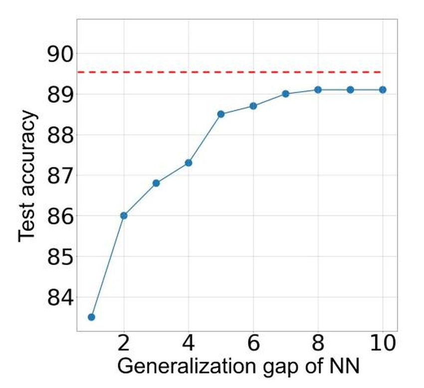
2        Authors Suppressed Due to Excessive Length

             (a) True Label Experiment                  (b) Random Label Experiment

            (c) IOC-AllConv (50% noise)                    (d) AllConv (50% noise)

Fig. 1. Training of AllConv and IOC-AllConv on CIFAR-10 dataset. (a) Loss curve while training
with true labels. AllConv starts overfitting after few epochs. IOC-AllConv does not exhibit over-
fitting, and the test loss nicely follows the training loss. (b) Accuracy plots while training with
randomized labels (labels were randomized for all the training images). If sufficiently trained,
even a simple network like MLP achieves 100% training accuracy and gives around 10% test ac-
curacy. IOC-MLP resists any learning on the randomized data and gives 0% generalization gap.
(c) and (d) Loss and accuracy plots on CIFAR-10 data when trained with 50% labels randomized
in the training set.

    We propose a principled and reliable alternative that tries to affirmatively resolve the
concerns raised in [31]. More specifically, we investigate a novel constrained family of
neural networks called Input Output Convex Neural Networks (IOC-NNs), which learn
a convex function between input and output. Convexity in machine learning typically
refers to convexity in terms of the parameters w.r.t to the loss [3], which is not the case
in our work. We use an IOC prefix to indicate the Input Output Convexity explicitly.
Amos et al. [1] have previously explored the idea of Input Output convexity; however,
their experiments limit to Partially Input Convex Neural Networks (PICNNs), where the
output is convex w.r.t some of the inputs. They deem fully convex networks unnecessary
in their studied setting of structured prediction, highly restricted on the allowable class
of models, highly limited, even failing to do simple identity mapping without additional
skip (pass-through) connections. Hence, they do not present even a single experiment
on fully convex networks.
    We wake this sleeping giant up and thoroughly investigate fully convex networks
(outputs are convex w.r.t to all the inputs) on the task of multi-class classification. Each
class in multi-class classification is represented as a convex function, and the resulting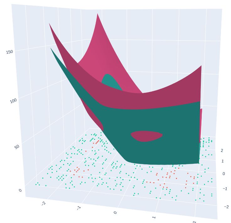
The Curious Case of Convex Neural Networks         3

decision boundaries are formed as an argmax of convex functions. Being able to train
IOC with NN-like capacity, we, for the first time, discover the beautiful underlying
properties, especially in terms of generalization abilities and robustness to label noise.
We investigate IOC-NNs on six commonly used image classification benchmarks and
pose them as a preferred alternative over the non-convex architectures. Our experiments
suggest that IOC-NNs avoid fitting over the noisy part of the data, in contrast to the
typical neural network behavior. Previous work shows that [2] neural networks tend
to learn simpler hypotheses first. Our experiments show that IOC-NNs tend to hold
on to the simpler hypothesis even in the presence of noise, without overfitting in most
settings.
     A motivating example is illustrated in Figure 1, where we train an All Convolu-
tional network (AllConv) [29] and its convex counterpart IOC-AllConv on the CIFAR-
10 dataset. AllConv starts overfitting the train data after a few epochs (Figure 1(a)). In
contrast, IOC-AllConv shows no signs of overfitting and flattens at the end (the test loss
values pleasantly follow the training curve). Such an observation is consistent across all
our experiments on IOC-NNs across different datasets and architectures, suggesting that
IOC-NNs have lesser reliance on explicit regularization like early stopping. Figure 1(b)
presents the accuracy plots for the randomized test where we train Multi-Layer Percep-
tron (MLP) and IOC-MLP on a copy of the data where the true labels were replaced by
random labels. MLP achieves 100% accuracy on the train set and gives a random chance
performance on the test set (observations are coherent with [31]). IOC-MLP resists any
learning and gives random chance performance (10% accuracy) on both train and test
sets. As MLP achieves zero training error, the test error is the same as generalization
error, i.e., 90% (the performance of random guessing on CIFAR10). In contrast, the
IOC-MLP has a near 0% generalization error. We further present experiment with 50%
noisy labels Figure 1(c). The neural network training profile concurs with the observa-
tion of Krueger et al. [18], where the network learns a simpler hypothesis first and then
starts memorizing. On the other hand, IOC-NN converges to the simpler hypothesis,
showing strong resistance to fit the noise labels.
     Input Output Convexity shows a promising paradigm, as any feed-forward network
can be re-worked into its convex counterpart by choosing a non-decreasing (and con-
vex) activation function and restricting its weights to be non-negative (for all but the
first layer). Our experiments suggest that activation functions that allow negative out-
puts (like leaky ReLU or ELU) are more suited for the task as they help retain negative
values flowing to subsequent layers in the network. We show that IOC-MLPs outper-
forms traditional MLPs in terms of test accuracy on five of the six studied datasets and
IOC-NNs almost recover the performance of the base network in case of convolutional
networks. In almost all studied scenarios, IOC networks achieve multi-fold improve-
ments in terms of generalization error over unconstrained Neural Networks. Overall,
our work makes the following contributions:

 – We bring to light the little known idea of Input Output Convexity in neural net-
   works. We propose a revised formulation to efficiently train IOC-NNs, retaining
   adequate capacity (with changes like using ELU, increasing nodes in the first layer,
   whitening transform at the input, etc.). To the best of our knowledge, we for the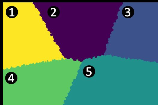
4         Authors Suppressed Due to Excessive Length

      first time explore a usable form of IOC-NNs, and shows that they can be trained
      with NN like capacity.
    – Through a set of intuitive experiments, we detail its internal functioning, especially
      in terms of its self regularization properties and decision boundaries. We show that
      how sufficiently complex decision boundaries can be learned using an argmax over
      a set of convex functions (where each class is represented by a single convex func-
      tion). We further propose a framework to learn the ensemble of IOC-NNs.
    – With a comprehensive set of quantitative and qualitative experiments, we demon-
      strate IOC-NN’s outstanding generalization abilities. IOC-MLPs achieve near zero
      generalization error in all the studied datasets and a negative generalization error
      (test accuracy is higher than train accuracy) in a couple of them, even at conver-
      gence. Such never seen behaviour opens up a promising avenue for more future
      explorations.
    – We explore the robustness of IOC-NNs to label noise and find that it strongly resists
      fitting the random labels. Even while training, IOC-NNs show no signs of fitting on
      noisy data and efficiently learns patterns from non noisy data. Our findings ignites
      explorations towards tighter generalization bounds for neural networks.

2     Related Work

Simple Convex models: Our work relates to parameter estimation on models that are
guaranteed to be convex by its construction. For regression problems, Magnani and
Boyd [20] study the problem of fitting a convex piecewise linear function to a given
set of data points. For classification problems, this traditionally translates to polyhe-
dral classifiers. A polyhedral classifier can be described as an intersection of a finite
number of hyperplanes. There have been several attempts to address the problem of
learning polyhedral classifiers [21, 15]. However, these algorithms require the number
of hyperplanes as an input, which is a major constraint. Furthermore, these classifiers do
not give completely smooth boundaries (at the intersection of hyperplanes). As another
major limitation, these classifiers cannot model the boundaries in which each class is
distributed over the union of non-intersecting convex regions (e.g., XOR problem). The
proposed IOC-NN (even with a single hidden layer) supersedes this direction of work.

Convex Neural Networks: Amos et al. [1] mentions the possibility of fully convex net-
works, however, does not present any experiments with it. The focus of their work is to
achieve structured predictions using partially convex network (using convexity w.r.t to
some of the inputs). They propose a specific architecture called FICNN which is fully
convex and has fully connected layers with skip connections. The skip connections are
a must because their architecture cannot even achieve identity mapping without them.
In contrast, our work can take any given architecture and derive its convex counter-
part (we use the IOC suffix to suggest model agnostic nature of our work). The work
by Kent et al. [16] analyze the links between polynomial functions and input convex
neural networks to understand the trade-offs between model expressiveness and ease
of optimization. Chen et al. [7, 8] explore the use of input convex neural network in a
variety of control applications like voltage regulation. The literature on input convex
The Curious Case of Convex Neural Networks 5
neural networks has been limited to niche tailored scenarios. Two key highlights of
our work are: (a) to use activations that allow the flow of negative values (like ELU,
leaky ReLU, etc.), which enables a richer representation (retaining fundamental prop-
erties like identity mapping which are not achievable using ReLU) and (b) to bring a
more in-depth perspective on the functioning of convex networks and the resulting de-
cision boundaries. Consequently, we present IOC-NNs as a preferred option over the
base architectures, especially in terms of generalization abilities, using experiments on
mainstream image classification benchmarks.
Generalization in Deep Neural Nets: Conventional machine learning wisdom says that
overparameterization leads to poor generalization performance owing to overfitting.
Counter-intuitively, empirical evidence shows that neural networks give better gener-
alization with an increased number of parameters even without any explicit regulariza-
tion [26]. Explaining how neural networks generalize despite being overparameterized
is an important question in deep learning [26, 23].
Neyshabur et al. [24] study different complexity measures and capacity bounds
based on the number of parameters, VC dimension, Rademacher complexity etc., and
conclude that these bounds fail to explain the generalization behavior of neural net-
works on overparameterization. Neyshabur et al. [25] suggest that restricting the hy-
pothesis class gives a generalization bound that decreases with an increase in the num-
ber of parameters. Their experiments show that restricting the spectral norm of the
hidden layer leads to tighter generalization bounds.
The above discussion implies that a hypothetical neural network that can fit any
hypothesis will have a worse generalization than the practical neural networks which
span a restricted hypothesis class. Inspired by this idea, we propose a principled way
of restricting the hypothesis class of neural networks (by convexity constraints) that
improves their generalization ability in practice. In the previous efforts to train fully
input output convex networks, they were shown to have a limited capacity compared to
its neural network counterpart [1, 3], making their generalization capabilities ineffective
in practice. To our knowledge, we for the first time present a method to formulate and
efficiently train IOC-NNs opening an avenue to explore their generalization ability.
3 Input Output Convex Networks
We first consider the case of an MLP with k hidden layers. The output of ith neuron
(l) (l)
in the lth hidden layer will be denoted as hi . For an input x = (x1 , . . . , xd ), hi is
defined as:
(l)
X (l) (l)
hi = φ( wij hl−1
j + bi ), (1)
j
(0) (k+1)
where, hj = xj (j = 1 . . . d) and hj = yj (j th output). The first hidden layer rep-
resents an affine mapping of input and preserves the convexity (i.e. each neuron in h(1)
is convex function of input). The subsequent layers are a weighted sum of neurons from
the previous layer followed by an activation function. The final output y is convex with
(2:k+1)
respect to the input x by ensuring two conditions: (a) wij ≥ 0 and (b) φ is convex6 Authors Suppressed Due to Excessive Length
and a non-decreasing function. The proof follows from the operator properties [5] that
the non-negative sum of convex functions is convex and the composition f (g(x)) is
convex if g is convex and f is convex and non-decreasing.
A similar intuition follows for convolutional architectures as well, where each neu-
ron in the next layer is a weighted sum of the previous layer. Convexity can be assured
by restricting filter weights to be non-negative and using a convex and non-decreasing
activation function. Filter weights in the first convolutional layer can take negative val-
ues, as they only represent an affine mapping of the input. The maxpool operation also
preserves convexity since point-wise maximum of convex functions is convex [5]. Also,
the skip connection does not violate Input Output Convexity, since the input to each
layer is still a non-negative weighted sum of convex functions.
We use an ELU activation to allow negative values; this is a minor but a key change
from the previous efforts that rely on ReLU activation. For instance, with non-negativity
(2:k+1)
constraints on weights (wij ≥ 0), ReLU activations restrict the allowable use of
hidden units that mirror the identity mapping. Previous works rely on passthrough/skip
connections to address [1] this concern. The use of ELU enables identity mapping and
allows us to use the convex counterparts of existing networks without any architectural
changes.
3.1 Convexity as Self Regularizer
We define self regularization as the property in which the network itself has some
functional constraints. Inducing convexity can be viewed as a self regularization tech-
nique. For example, consider a quadratic classifier in R2 of the form f (x1 , x2 ) =
w1 x21 + w2 x22 + w3 x1 x2 + w4 x1 + w5 x2 + w0 . If we want the function f to be convex,
then it is required that the network imposes following constraints on the parameters,
√ √
w1 ≥ 0, w2 ≥ 0, −2 w1 w2 ≤ w3 ≤ 2 w1 w2 , which essentially means that we are
restricting the hypothesis space.
Similar inferences can be drawn by taking the example of polyhedral classifiers.
Polyhedral classifiers are a special class of Mixture of Experts (MoE) network [13,
27]. VC-dimension of a polyhedral classifier in d-dimension formed by the intersection
of m hyperplanes is upper bounded by 2(d + 1)m log(3m) [30]. On the other hand,
VC-dimension of a standard mixture of m binary experts in d-dimension is O(m4 d2 )
[14]. Thus, by imposing convexity, the VC-dimension becomes linear with the data
dimension d and m log(m) with the number of experts. This is a huge reduction in the
overall representation capacity compared to the standard mixture of binary experts.
Furthermore, adding non-negativity constraints alone can lead to regularization. For
example, the VC dimension of a sign constrained linear classifier in Rd reduces from
d + 1 to d [6, 19]. The proposed IOC-NN uses a combination of sign constraints and
restrictions on the family of activation functions for inducing convexity. The representa-
tion capacity of the resulting network reduces, and therefore, regularization comes into
effect. This effectively helps in improving generalization and controlling overfitting, as
clearly observed in our empirical studies (Section 4.1).The Curious Case of Convex Neural Networks 7
(a) (b) (c) (d)
Fig. 2. Decision boundaries of different networks trained for two class classification. (a) Original
data: one class shown by blue and the other orange. (b) Decision boundary learnt using MLP.
(c) Decision boundary learnt using IOC-MLP with single node in the output layer. (d) Decision
boundary learnt using IOC-MLP with two nodes in the output layer (ground truth as one hot
vectors)
.
f(x)
g(x)
C2 C1 C2 C1 C2 C1 C2
(a) (b)
Fig. 3. (a) Using two simple 1-D functions we illustrate that argmax of two convex functions
can result into non-convex decision boundaries. (b) Two convex functions whose argmax results
into the decision boundaries shown in Figure 2(d). The same plot is shown from two different
viewpoints.
3.2 IOC-NN Decision Boundaries
Consider a scenario of binary classification in 2D space as presented in Figure 2(a).
We train a three-layer MLP with a single output and a sigmoid activation for the last
layer. The network comfortably learns to separate the two classes. The learned bound-
aries by the MLP are shown in Figure 2(b). We then train an IOC-MLP with the same
architecture. The learned boundary is shown in Figure 2(c). IOC-MLP learns a single
convex function as output w.r.t the input and its contour at the value of 0.5 define the
decision boundary. The use of non-convex activation like sigmoid in the last layer does
not distort convexity of decision boundary (Appendix A)
We further explore IOC-MLP with a variant architecture where the ground truth
is presented as a one-hot vector (allowing two outputs). The network learns two con-
vex functions f and g representing each class, and their argmax defines the decision
boundary. Thus, if g(x) − f (x) > 0, then x is assigned to class C1 and C2 otherwise.
Therefore, it can learn non-convex decision boundaries as shown in Figure 3. Please
note that g − f is no more convex unless g 00 − f 00 ≥ 0. In the considered problem
of binary classification in Figure 2, using one-hot output allows the network to learn
non-convex boundaries (Figure 2 (d)). The corresponding two output functions (one8 Authors Suppressed Due to Excessive Length
(a) (b) (c)
Fig. 4. (a) Original Data. (b) Output of the gating network, each color represents picking a partic-
ular expert. (c) Decision boundaries of the individual IOC-MLPs. We mark the correspondences
between each expert and the segment for which it was selected. Notice how the V-shape is parti-
tioned and classified using two different IOC-MLPs.
for each class) are illustrated in Figure 3 (b). We can observe that both the individ-
ual functions are convex; however, their arrangement is such that the argmax leads
to a reasonably complex decision boundary.This happens due to the fact that the sets
S1 = {x | g(x) − f (x) > 0} and S2 = {x | g(x) − f (x) ≤ 0} can both be non-convex
(even though functions f (.) and g(.) are convex).
3.3 Ensemble of IOC-NN
We further explore the ensemble of IOC-NN for multi-class classification. We explore
two different ways to learn the ensembles:
1. Mixture of IOC-NN Experts: Training a mixture of IOC-NNs and an additional
gating network [13]. The gating network can be non-convex and outputs a scalar
weight for each expert. The gating network and the multiple IOC-NNs (experts) are
trained in an Expectation-Maximization (EM) framework, i.e., training the gating
network and the experts iteratively.
2. Boosting + Gating: In this setup, each IOC-NN is trained individually. The first
model is trained on the whole data, and the consecutive models are trained with
exaggerated data on the samples on which the previous model performs poorly. For
bootstrapping, we use a simple re-weighting mechanism as in [10]. A gating net-
work is then trained over the ensemble of IOC-NNs. The weights of the individual
networks are frozen while training the gating network.
We detail the idea of ensembles using a representative experiment for binary classi-
fication on the data presented in Figure 4(a). We train a mixture of p IOC-MLPs with
a gating network using the EM algorithm. The gating network is an MLP with a single
hidden layer, the output of which is a p dimensional vector. Each of the IOC-MLP is a
three-layer MLP with a single output. We keep a single output to ensure that each IOC-
MLP learns a convex decision boundary. The output of the gating network is illustrated
in Figure 4(b). A particular IOC-MLP was selected for each partition and led to five
partitions. The decision boundaries of individual IOC-MLPs are shown in Figure 4(c).
It is interesting to note that the MoE of binary IOC-MLPs fractures the input space into
sub-spaces where a convex boundary is sufficient for classification.The Curious Case of Convex Neural Networks 9
4 Experiments
Dataset and Architectures: To show the significance of enhanced performance of IOC-
MLP over traditional NN, we train them on six different datasets: MNIST, FMNIST,
STL-10, SVHN, CIFAR-10, and CIFAR-100. We use an MLP with three hidden layers
and 800 nodes in each layer. We use batch normalization between every layer, and it’s
activation in all hidden layers. ReLU and ELU are used as activations for NN and IOC
respectively, and softmax is used in the last layer. We use Adam optimizer with an initial
learning rate of 0.0001 and use validation accuracy for early stopping.
We perform experiments that involve two additional architectures to extend the
comparative study between IOC and NN on CIFAR-10 and CIFAR-100 datasets. We
use a fully convolutional [29], and a densely connected architecture [12]. We choose
DenseNet with growth rate k=12, for our experiments. We term the convex counterparts
as IOC-AllConv, IOC-DenseNet, respectively, and compare against their base neural
network counterparts [12, 29]. In all comparative studies, we follow the same training
and augmentation strategy to train IOC-NNs, as used by the aforementioned neural
networks.
Training on duplicate free data: The test sets of CIFAR-10 and CIFAR-100 datasets
have 3.25% and 10% duplicate images, respectively [4]. Neural networks show higher
performance on these datasets due to the bias created by this duplicate data (neural net-
works have been shown to memorize the data). CIFAIR-10 and CIFAIR-100 datasets
are variants of CIFAR-10 and CIFAR-100 respectively, where all the duplicate images
in the test data are replaced with new images. Barz et al. [4] observed that the perfor-
mance of most neural architectures drops when trained and tested on bias-free CIFAIR
data. We train IOC-NN and their neural network counterparts on CIFAIR-10 data with
three different architectures: a fully connected network (MLP), a fully convolutional
network (AllConv) [29] and a densely connected network (DenseNet) [12].
Training IOC architectures: We tried four variations for weight constraints to enforce
convexity constraints: clipping negative weights to zero, taking absolute of weights,
exponentiation of negative weights and shifting the weights after each iteration. We use
exponentiation strategy in all experiments, as it gave the best results. We exponentiate
the negative weights after every update. The IOC constrained optimization algorithm
differs only by a single step from the traditional algorithms (Appendix B).
To conserve convexity in the batch-normalization layer, we also constrain the gamma
scaler with exponentiation. However, in practice we found that the IOC networks retains
all desirable properties without constraining the gamma scalar. We make few additional
modifications to facilitate the training of IOC-NNs. Such changes do not affect the per-
formance of the base neural networks. We use ELU as an activation function instead
of ReLU in IOC-NNs. We apply the whitening transformation to the input so that it
is zero-centered, decorrelated, and spans over positive and negative values equally. We
also increase the number of nodes in the first layer (the only layer where parameters can
take negative values). We use a slower schedule for learning rate decay than the base
counterparts. The IOC-NNs have a softmax layer at the last layer and are trained with
cross-entropy loss (same as neural networks).10 Authors Suppressed Due to Excessive Length
Training ensembles of binary experts: We divide CIFAR-10 dataset into 2 classes,
namely: ‘Animal’ (CIFAR-10 labels: ‘Bird’, ‘Cat’, ‘Deer’, ‘Dog’, ‘Frog’ and ‘Horse’)
and ‘Not Animal’. We train an ensemble of IOC-MLP, where each expert is a three-
layer MLP with one output (with sigmoid activation at the output node). The gating
network in the EM approach is a one layer MLP which takes an image as input and
predicts the weights by which the individual expert predictions get averaged. We report
test results of ensembles with each additional expert. This experiment resembles the
study shown in Figure 4.
Training Boosted ensembles: The lower training accuracy of IOC-NNs makes them
suitable for boosting (while the training accuracy saturates in non-convex counterparts).
For bootstrapping, we use a simple re-weighting mechanism as in [10]. We train three
experts for each experiment. The gating network is a regular neural network, which is
a shallow version of the actual experts. We train an MLP with only one hidden layer,
a four-layer fully convolutional network, and a DenseNet with two dense-blocks as
the gate for the three respective architectures. We report the accuracy of the ensemble
trained in this fashion as well as the accuracy if we would have used an oracle instead
of the gating network.
Partially randomized labeling: Here, we investigate IOC-NN’s behavior in the pres-
ence of partial label noise. We do a comparative study between IOC and neural net-
works using All-Conv architecture, similar to the experiment performed by [31]. We
use CIFAR-10 dataset and make them noisy by systematically randomizing the labels
of a selected percentage of training data. We report the performance of All-Conv, and
it’s IOC counterpart on 20, 40, 60, 80 and 100 percent noise in the train data. We report
train and test scores at peak performance (performance if we had used early stopping)
and at convergence (if loss goes below 0.001 or at 2000 epochs).
4.1 Results
IOC as a preferred alternative for Multi-Layer-Perceptrons: MLP is most basic and
earliest explored form of neural networks. We compare the train and test scores of
MLP and IOC-MLP in Table 1. With a sufficient number of parameters, MLP (a basic
NN architecture) perfectly fits the training data. However, it fails to generalize well
on the test data owing to brute force memorization. The results in Table 1 indicate
that IOC-MLP gives a smaller generalization gap (the difference between train and test
accuracies) compared to MLP. The generalization gap even goes to negative values
on three of the datasets. MLP (being poorly optimized for parameter utilization) is
one of the architectures prone to overfitting the most, and IOC constraints help retain
test performance resisting the tendency to overfit. Obtaining negative or almost zero
generalization error even at convergence is a never seen behaviour in deep networks
and the results clearly suggest the profound generalization abilities of Input Output
Convexity, especially when applied to fully connected networks.
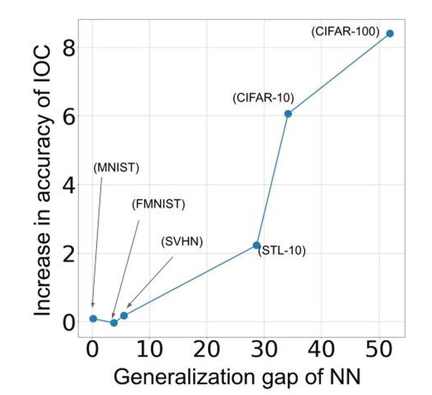
Furthermore, having the IOC constraints significantly boosts the test accuracy on
datasets where neural network gives a high generalization gap (Table 1). This trend
is clearly visible in Figure 5(b). For the CIFAR-10 dataset, unconstrained MLP givesThe Curious Case of Convex Neural Networks 11
NN IOC-NN
train test gen. gap train test gen. gap
MNIST 99.34 99.16 0.19 98.77 99.25 -0.48
FMNIST 94.8 90.61 3.81 90.41 90.58 -0.02
STL-10 81 52.32 28.68 62.3 54.55 7.75
SVHN 91.76 86.19 5.57 81.18 86.37 -5.19
CIFAR-10 97.99 63.83 34.16 73.27 69.89 3.38
CIFAR-100 84.6 32.68 51.92 46.9 41.08 5.82
Table 1. Table shows train accuracy, test accuracy and generalization gap for MLP and IOC-MLP
on six different datasets.
CIFAR-10 CIFAR-100
NN IOC-NN NN IOC-NN
train test gen. gap train test gen. gap train test gen. gap train test gen. gap
MLP 99.17 63.83 35.34 73.27 69.89 3.3 84.6 32.68 51.9 46.9 41.08 5.8
AllConv 99.31 92.8 6.5 93.2 90.6 2.6 97.87 69.5 28.4 67.07 65.08 1.9
DenseNet 99.46 94.06 5.4 94.22 91.12 3.1 98.42 75.36 23.06 74.9 68.53 6.3
Table 2. Train accuracy, test accuracy and generalization gap of three neural architectures and
their IOC counterparts
34.16% generalization gap, while IOC-NN brings down the generalization gap by more
than ten folds and boosts the test performance by about 6%. Even in scenarios where
neural networks give a smaller generalization gap (like MNIST and SVHN), IOC-NN
marginally outperforms regular NN and gives an advantage in generalization. Overall,
the results in Table 1 highlight that IOC constraints are extremely beneficial when train-
ing Multi Layer Perceptrons for image classification, giving comprehensive advantages
in terms of generalization and test performance.
Better generalization: We investigate the generalization capability of IOC-NN on other
architectures. The results of the base architectures and their convex counterparts on
CIFAR-10 and CIFAR-100 datasets are presented in Table 2. IOC-NN outperforms base
NN on MLP architecture and gives comparable test accuracies for convolutional archi-
tectures. The train accuracies are saturated in the base networks (reaching above 99%
in most experiments). The lower train accuracy in IOC-NNs suggests that there might
still be room for improvement, possibly through better design choices tailored for IOC-
NNs. In Table 2, the difference in train and test accuracy across all the architectures
(generalization gap) demonstrates the better generalization ability of IOC-NNs. The
generalization gap of base architectures is at least twofold more than IOC-NNs on the
CIFAR-100 dataset. For instance, the generalization error of IOC-AllConv on CIFAR-
100 is only 1.99%, in contrast to 28.4% in AllConv. The generalization ability of IOC-
NNs is further qualitatively reflected using the training and validation loss profiles (e.g.,
Figure1(a)). We present a table showing the confidence intervals of prediction across all
three architectures with repeated runs in Appendix C.
Table 5 shows the train and test performance of the three architectures on CIFAR-
10 dataset and the drop incurred when trained on CIFAIR-10. The drop in test perfor-12 Authors Suppressed Due to Excessive Length
NN IOC-NN
peak convergence peak convergence
train test train test gen. gap train test train test gen. gap
100 98.63 10.53 97.80 10.1 87.7 9.98 10.62 10.21 9.94 0.27
80 22.40 60.24 97.83 27.75 70.08 21.93 61.48 23.80 56.20 -32.4
60 38.52 75.80 97.80 46.71 51.09 37.90 75.91 39.31 71.75 -32.44
40 56.48 80.47 97.96 61.83 36.13 55.01 81.58 54.63 81.01 -26.38
20 72.8 85.72 98.73 76.31 22.42 69.92 85.85 70.22 83.61 -13.39
Table 3. Results for systematically randomized labels at peak and at convergence for both IOC-
NN and NN. The IOC constraints bring huge improvements in generalization error and test accu-
racy at convergence.
Base MLP Constrained MLP FICNN IOC-NN
train 99.17 46.81 62.8 73.27
test 63.83 27.36 53.07 69.89
gen-gap 35.34 19.45 9.73 3.38
Table 4. Results comparing FICNN [1] with IOC-NN on CIFAR-10 using MLP architecture. First
column shows base MLP results. Second column presents results with a convex MLP using ReLU
activation. Third and final columns show the accuracies of FICNN and IOC-NN, respectively.
mance of IOC-NNs is smaller than the typical neural network. This further strengthens
the claim that IOC-NNs are not memorizing the training data but learning a generic
hypothesis.
Comparison with FICNN: Table 4 shows the results of IOC-NN and FICNN [1] on
CIFAR-10 data. For comparison, we use a three layer MLP with 800 nodes in each
layer, for both IOC-NN and FICNN. FICNN uses a skip connection from input layer to
each of the intermittent layers. This enables each layer to learn identity mapping inspite
of non-negative constraint. The number of parameters in FICNN model is almost twice
compared to the base MLP and IOC models but still the test performance drops by more
than 10%. The results clearly shows that IOC-NN gives better test accuracy and lower
generalization gap compared to FICNN, while using the same number of parameters as
the base MLP architecture.
Robustness to random label noise: Robustness of IOC-NNs on partial and fully ran-
domized labels (Figure 1 (b, c, and d)) is one of its key properties. We further investigate
this property by systematically randomizing increasing portion of labels. We report the
results of neural networks and their convex counterparts with percentage of label noise
varying from 20% to 100% in Table 3. The train performance of neural networks at
convergence is near 100% across all noise levels. It is interesting to note that IOC-NN
gives a large negative generalization gap, where the train accuracy is almost equal to the
percentage of true labels in the data. This observation shows that IOC-NNs significantly
resist learning noise in labels as compared to neural networks. Both neural network and
it’s convex counterpart learns the simple hypothesis first. While IOC-NN holds on toThe Curious Case of Convex Neural Networks 13
NN IOC-NN
C-10 CIFAIR Gap C-10 CIFAIR Gap
MLP 63.6 63.08 0.52 69.89 69.51 0.38
AllConv 92.8 91.14 0.66 90.6 90.47 0.13
DenseNet 94.06 93.28 0.78 91.12 90.73 0.39
Table 5. Results on CIFAIR-10 dataset
(a) (b)
Fig. 5. (a) shows the test accuracy of IOC-MLP with increasing number of experts in the binary
classification setting. Average performance of normal MLP is shown in red since it does not
change with increase in number of experts. (b) The generalization gap of MLP plotted against the
improvement gained by the IOC-MLP for the six different datasets (represented by every point on
the plot). The performance gain with IOC constraints increase with the increase in generalization
gap of MLP.
this, in later epochs, the neural network starts brute force memorization of noisy labels.
The observations are coherent with findings in [18, 28], demonstrating neural network’s
heavy reliance on early stopping. IOC-AllConv outperforms test accuracy of AllConv
+ early stopping with a much-coveted generalization behavior. It is clear from this ex-
periment that IOC-NN performs better in the presence of random label noise in the data
in terms of test accuracy both at peak and convergence.
Leverage IOC properties to train ensembles: We train binary MoE on the modified two-
class setting of CIFAR-10 as described in Section 4. The result is shown in Figure 5 (a).
Traditional neural network gives a test accuracy of 89.63% with a generalization gap
of 10%. Gated MoE of NNs does not improve the test performance as we increase the
number of experts. In contrast, the performance of ensemble of IOC-NNs goes up with
the addition of each expert and moves closer to the performance of neural networks. It
is interesting to note that even in the higher dimensional space (like CIFAR-10 images),
the intuitions derived from Figure 4 holds. We also note that gate fractures the space
into p partitions (where p is the number of experts). Moreover, in the binary case for a
single expert, the generalization gap is almost zero. This can be attributed to the convex
hull like smooth decision boundary that the network predicts in the binary setting with
a single output.14 Authors Suppressed Due to Excessive Length
single expert gate oracle
MLP 69.89 71.8 85.47
All-Conv 90.6 92.83 96.3
DenseNet 91.12 93.25 97.19
Table 6. Result for single expert, gated MoE and with oracle on CIFAR-10 for three architectures
(a) MLP (b) AllConv (c) DenseNet
Fig. 6. These diagrams show expected sample accuracy as a function of confidence [9]. The blue
bar shows the confidence of the bin and the orange bar shows the percentage correctness of
prediction in that bin. If the model is perfectly calibrated, the bars align to form identity function.
Any deviation from a perfect diagonal is a miscalibration.
The results with the boosted ensembles of IOC-NNs are presented in Table 6. The
boosted ensemble improves the test accuracies of IOC-NNs, matching or outperforming
the base architectures. However, this performance gain comes at the cost of increased
generalization error (still lower than the base architectures). In the boosted ensemble,
the performance significantly improves if the gating network is replaced by an oracle.
This observation suggests that there is a scope of improvement in model selection abil-
ity, possibly by using a better gating architecture.
Confidence Calibration of IOC-NNs: In a classification setting, given an input, the
neural network predicts probability-like scores towards each class. The class with the
maximum score is considered the predicted output, and the corresponding score to be
the confidence. The confidence and accuracy being correlated is a desirable property,
especially in high-risk applications like self-driving cars, medical diagnoses, etc. How-
ever, many modern multi-class classification networks are poorly calibrated, i.e., the
probability values that they associate with the class labels they predict overestimate the
likelihoods of those class labels being correct in the real world [11]. Recent works have
explored methods to improve the calibration of neural networks [11, 22].
We observe that adding IOC constraints improve calibration error on the base NN ar-
chitecture. We present the reliability diagrams [9] (presenting accuracy as a function of
confidence) of three neural architectures and their convex counterparts in Figure 6. The
sum of the difference between the blue bars and the orange bars represents the Expected
Calibration Error. IOC constraints show improved calibration in all three architectures
(with notable improvements in the case of MLP and AllConv). Better calibration further
strengthens the case for IOC-NNs from the application perspective.The Curious Case of Convex Neural Networks 15
5 Conclusions
We present a subclass of neural networks, where the output is a convex function of the
input. We show that with minimal constraints, existing neural networks can be adopted
to this subclass called Input Output Convex Neural Networks. With a set of carefully
chosen experiments, we unveil that IOC-NNs show outstanding generalization ability
and robustness to label noise while retaining adequate capacity. We show that in sce-
narios where the neural network gives a large generalization gap, IOC-NN can give
better test performance. An alternate interpretation of our work can be self regulariza-
tion (regularization through functional constraints). IOC-NN puts to rest the concerns
around brute force memorization of deep neural networks and opens a promising hori-
zon for the community to explore. We show that in the case of Multi-Layer-Perceptrons,
IOC constraints improve accuracy, generalization, calibration, and robustness to noise,
making an ideal proposition from a deployment perspective. The improved generaliza-
tion, calibration, and robustness to noise are also observed in convolutional architectures
while retaining the accuracy. In future work, we plan to investigate the use of IOC-NNs
for recurrent architectures. Furthermore, we plan to explore the interpretability aspects
of IOC-NNs and study the effect of convexity constraints on the generalization bounds.
References
1. Brandon Amos, Lei Xu, and J Zico Kolter. Input convex neural networks. In Proceedings of
the 34th International Conference on Machine Learning-Volume 70, pages 146–155. JMLR.
org, 2017.
2. Devansh Arpit, Stanislaw Jastrzebski, Nicolas Ballas, David Krueger, Emmanuel Bengio,
Maxinder S Kanwal, Tegan Maharaj, Asja Fischer, Aaron Courville, Yoshua Bengio, et al.
A closer look at memorization in deep networks. In International Conference on Machine
Learning, pages 233–242. PMLR, 2017.
3. Francis Bach. Breaking the curse of dimensionality with convex neural networks. The
Journal of Machine Learning Research, 18(1):629–681, 2017.
4. Björn Barz and Joachim Denzler. Do we train on test data? purging cifar of near-duplicates.
Journal of Imaging, 6:41, 06 2020.
5. Stephen Boyd, Stephen P Boyd, and Lieven Vandenberghe. Convex optimization. Cambridge
university press, 2004.
6. Chris J.C. Burges. A tutorial on support vector machines for pattern recognition. Data
Mining and Knowledge Discovery, 2:121–167, January 1998.
7. Yize Chen, Yuanyuan Shi, and Baosen Zhang. Optimal control via neural networks: A con-
vex approach. arXiv preprint arXiv:1805.11835, 2018.
8. Yize Chen, Yuanyuan Shi, and Baosen Zhang. Input convex neural networks for optimal
voltage regulation. arXiv preprint arXiv:2002.08684, 2020.
9. Morris H DeGroot and Stephen E. Fienberg. The comparison and evaluation of forecasters.
The statistician, pages 12–22, 1983.
10. Jerome Friedman, Trevor Hastie, Robert Tibshirani, et al. Additive logistic regression: a
statistical view of boosting (with discussion and a rejoinder by the authors). The annals of
statistics, 28(2):337–407, 2000.
11. Chuan Guo, Geoff Pleiss, Yu Sun, and Kilian Weinberger. On calibration of modern neural
networks. arXiv preprint arXiv:1706.04599, 06 2017.16 Authors Suppressed Due to Excessive Length
12. Gao Huang, Zhuang Liu, Laurens van der Maaten, and Kilian Q Weinberger. Densely con-
nected convolutional networks. In Proceedings of the IEEE Conference on Computer Vision
and Pattern Recognition, 2017.
13. Robert A. Jacobs, Michael I. Jordan, Steven J. Nowlan, and Geoffrey E. Hinton. Adaptive
mixtures of local experts. Neural Comput., 3(1):79–87, March 1991.
14. Wenxin Jiang. The vc dimension for mixtures of binary classifiers. Neural Computation,
12(6):1293–1301, 2000.
15. Alex Kantchelian, Michael C Tschantz, Ling Huang, Peter L Bartlett, Anthony D Joseph,
and J. D. Tygar. Large-margin convex polytope machine. In Advances in Neural Information
Processing Systems 27, pages 3248–3256. Curran Associates, Inc., 2014.
16. Spencer Kent, Eric Mazumdar, Anusha Nagabandi, and Kate Rakelly. Input-convex neural
networks and posynomial optimization, 2016.
17. Anita Kripfganz and R. Schulze. Piecewise affine functions as a difference of two convex
functions. Optimization, 18(1):23–29, 1987.
18. David Krueger, Nicolas Ballas, Stanislaw Jastrzebski, Devansh Arpit, Maxinder S Kanwal,
Tegan Maharaj, Emmanuel Bengio, Asja Fischer, and Aaron Courville. Deep nets don’t learn
via memorization, 2017.
19. Robert Legenstein and Wolfgang Maass. On the classification capability of sign-constrained
perceptrons. Neural Computation, 20(1):288–309, 2008.
20. Alessandro Magnani and Stephen P Boyd. Convex piecewise-linear fitting. Optimization
and Engineering, 10(1):1–17, 2009.
21. Naresh Manwani and PS Sastry. Learning polyhedral classifiers using logistic function. In
Proceedings of 2nd Asian Conference on Machine Learning, pages 17–30, 2010.
22. Jishnu Mukhoti, Viveka Kulharia, Amartya Sanyal, Stuart Golodetz, Philip Torr, and
Puneet Dokania. Calibrating deep neural networks using focal loss. arXiv preprint
arXiv:2002.09437, 02 2020.
23. Vaishnavh Nagarajan and J. Kolter. Uniform convergence may be unable to explain general-
ization in deep learning. arXiv preprint arXiv:1902.04742, 02 2019.
24. Behnam Neyshabur, Srinadh Bhojanapalli, David McAllester, and Nati Srebro. Exploring
generalization in deep learning. In Advances in Neural Information Processing Systems,
pages 5947–5956, 2017.
25. Behnam Neyshabur, Zhiyuan Li, Srinadh Bhojanapalli, Yann LeCun, and Nathan Srebro.
Towards understanding the role of over-parametrization in generalization of neural networks.
arXiv preprint arXiv: 1805.12076, 05 2018.
26. Behnam Neyshabur, Ryota Tomioka, and Nathan Srebro. In search of the real inductive bias:
On the role of implicit regularization in deep learning. arXiv preprint arXiv:1412.6614, 12
2014.
27. Kulin Shah, PS Sastry, and Naresh Manwani. Plume: Polyhedral learning using mixture of
experts. arXiv preprint arXiv:1904.09948, 2019.
28. Jonas Sjöberg and Lennart Ljung. Overtraining, regularization and searching for a minimum,
with application to neural networks. International Journal of Control, 62(6):1391–1407,
1995.
29. Jost Tobias Springenberg, Alexey Dosovitskiy, Thomas Brox, and Martin Riedmiller. Striv-
ing for simplicity: The all convolutional net. arXiv preprint arXiv:1412.6806, 2014.
30. Gábor Takács and Béla Pataki. Lower bounds on the vapnik-chervonenkis dimension of con-
vex polytope classifiers. In 2007 11th International Conference on Intelligent Engineering
Systems, pages 145 – 148, 06 2007.
31. Chiyuan Zhang, Samy Bengio, Moritz Hardt, Benjamin Recht, and Oriol Vinyals. Under-
standing deep learning requires rethinking generalization. arXiv preprint arXiv:1611.03530,
2016.Appendix
This document contains the supplementary material to support the main text. The
contents of this document are:
– Appendix A: Using non-convex activations in the last layer of Input Output Convex
Neural Networks (IOC-NNs)
– Appendix B: Optimization algorithm for training IOC-NNs
– Appendix C: Table showing confidence intervals of IOC-NNs and their neural net-
work counterparts
– Appendix D: Discussion on Capacity of IOC-NNs
– Appendix E: Partition of input space by MoEs of IOC-NNs
A Using Non-Convex Activations to Facilitate Training
In a multi-class classification setting, the softmax function is widely used to get a joint
probability distribution over the output classes. This facilitates training with categorical
cross-entropy loss. The softmax layer distorts input output convexity, but the decision
boundary remains unchanged even after applying softmax in the last layer. Each of the
pre-softmax output of IOC-NNs is convex with respect to the inputs. The classifica-
tion decision is determined by the order (rank) of these values, as this rank remains
unaffected with the application of the softmax function. At inference time, we compute
argmax of convex functions (pre-softmax layer).
argmax(Y ) = argmax(sof tmax(Y )) (1)
A similar approach is taken for modelling independent probabilities of labels in binary
classification setting. Sigmoid activation is widely used to model the probability p(y =
yn |x). For IOC-NN, at inference, the predicted value is y = σ(f (x)), where f (x) is
convex. Hence, decision boundary is:
σ(f (x)) = 0.5, (2)
which is equivalent to
f (x) = σ −1 (0.5) (3)
−1
where, f (x) is convex. Since σ (0.5) is a constant, the decision boundary is convex.
B Optimization Algorithm for Training IOC-NNs
The only architectural constraint in designing an IOC-NN is the choice of a convex and
non-decreasing activation function. Furthermore, any feed-forward neural architecture
can be trained as IOC-NN by adding two steps to the optimization algorithm. For ex-
ample, the constrained version of the vanilla stochastic gradient descent algorithm is
shown in Algorithm 1.
is used to bring down the value of the updated weights post exponentiation for
negative values close to zero. Values near zero, post exponentiation, will be close to one,18
Algorithm 1: Algorithm to train a k layer IOC-NN
Input: Training data S, Labels L, learning rate η, constant , θ0 = (w0 n n
ij , b0 i )
Output: Θ = (w∗ , b∗ )
initialize: θ = θ0 ;
while stopping criteria not met do
for i in 1:len(S) / batch size do
sample(xbatch , ybatch ) ∈ (S, L);
L ← Div(fθ (xbatch ), ybatch );
∂
w ← w − η( ∂w L);
∂
b ← b − η( ∂b L);
for layer ∈ 2 : k do
if w < 0 then
w ← ew− ;
end
end
end
check stopping criteria
end
Table 1. .
NN IOC-NN
train test Gen. error train test Gen. error
MLP 97.99 ± 0.18 63.83 ± 0.12 34.1 73.27 ± 0.41 69.89 ± 0.21 3.38
All Conv 99.12 ± 1.03 92.21 ± 0.18 7.09 92.61 ± 1.45 90.34 ± 0.20 2.27
DenseNet 99.08 ± 0.75 93.86 ± 0.46 5.22 93.8 ± 0.83 90.43 ± 0.59 3.37
and helps keep them close to zero. We use = 5 across all experiments. To summarize,
the only two additional steps required to train an IOC-NN are condition (to check the
sign of updated weights) and exponentiation. We can develop IOC constrained versions
for all optimization algorithms that are used in training neural networks.
C Confidence Intervals of Classification Accuracies for Neural
Networks and IOC-NNs
We run MLP, AllConv and Densenet on CIFAR-10 data five times. We report the accu-
racy in prediction and the confidence intervals obtained over five runs in Table 1. We
report the train and test accuracies along with the generalization gap. The table confirms
the reliability of the results in the main document. The generalization gap of IOC-NNs
are consistently lower than neural networks. Also, compared to base MLP the convex
counterpart gives higher test accuracy.Appendix 19 D Discussion on Capacity of IOC-NNs The decision boundaries of real-world classification problems are often not convex. Each of the single outputs of IOC-NN is convex with respect to the inputs by design. However, it can still learn arbitrarily complex decision boundaries. Kripfganz et al.[17] show that we can represent any piecewise linear function as a difference of two piece- wise linear convex functions. Using ReLU as an activation limits the function classes that convex networks can learn. For instance, they cannot learn identity mapping [1]. A simple architectural change of using ELU overcomes this issue and hence increases the capacity of IOC-NNs. Results in the main text show empirical evidence of this increase in capacity. Following this direction in the future, we would like to explore the proof for universal approximation for IOC-NNs. Fig. 1. The figure shows the mean image of ten clusters within the class ’Automobile’. Each cluster corresponds to the expert picked by the gate. These partitions signify the difference in the data points on which each of the binary convex models gained expertise. E Partition of Input space by MoEs of IOC-NNs Real-world data often lies in a sparse, high-dimensional space and neural networks fit complex boundaries on them. These complex boundaries make the classification results challenging to interpret. In section 3.2 of the main text, we demonstrate on toy data, how an ensemble of binary IOC-NNs creates meaningful partitions of input space. Gat- ing network of MoEs of IOC-NNs partition input space into mutually exclusive and ex- haustive subspaces. The partition chosen by the gate for each expert is a portion where a convex boundary is enough to make a reasonable prediction. We train ten, three layered single output IOC-MLPs using gated EM strategy on the two-class setting of CIFAR-10 as explained in section 4: ’Training ensembles of binary experts’. Figure 1 shows the mean image of ten partitions of class ’Automobile’. Each partition corresponds to one of the ten experts chosen by the gate. Each of the IOC-NN has expertise on clusters with aspects that can lead to some real-world interpretation. For instance, an expert is
20

chosen by the gate to classify images showing the front view of red cars from similar
images, while another expert is picked for side view images. Similar clusters can be
seen corresponding to different colors and orientations. In the future, we would like to
explore this property of MoE of binary IOC-NNs towards improving the interpretability
of decisions made by neural networks.
You can also read