Streaming saturation for large RDF graphs with dynamic schema information - LAMSADE
←
→
Page content transcription
If your browser does not render page correctly, please read the page content below
Streaming saturation for large RDF graphs
           with dynamic schema information

Mohammad Amin Farvardin1 , Dario Colazzo1 , Khalid Belhajjame1 and Carlo
                              Sartiani2

    Université Paris-Dauphine, Place du Maréchal de Lattre de Tassigny, 75016 Paris,
          [mohammad-amin.farvardin, dario.colazzo, khalid.belhajjame]
                                   @lamsade.dauphine.fr
            Università della Basilicata,Via dell’Ateneo Lucano, Potenza, Italy,
                                carlo.sartiani@unibas.it

         Abstract. In the Big Data era, RDF data are produced in high vol-
         umes. While there exist proposals for reasoning over large RDF graphs
         using big data platforms, there is a dearth of solutions that do so in en-
         vironments where RDF data are dynamic, and where new instance and
         schema triples can arrive at any time. In this work, we present the first
         solution for reasoning over large streams of RDF data using big data
         platforms. In doing so, we focus on the saturation operation, which seek
         to infer implicit RDF triples given RDF schema constraints. Indeed, un-
         like existing solutions which saturate RDF data in bulk, our solution
         carefully identifies the fragment of the existing (and already saturated)
         RDF dataset that needs to be considered given the fresh RDF state-
         ments delivered by the stream. Thereby, it performs the saturation in an
         incremental manner. An experimental analysis shows that our solution
         outperforms existing bulk-based saturation solutions.

     Keywords: RDF saturation, RDF streams, Big Data, Spark

1      Introduction

To take full advantage of semantic data and turn them into actionable knowledge,
the semantic web community has devised techniques for processing and reasoning
over RDF data (e.g. [4, 18, 22]). However, in the Big Data era, RDF data, just
like many other kinds of data, are produced in high volumes. This is partly due
to sensor data produced in the context of health monitoring and financial market
applications, feeds of user-content provided by social network platforms, as well
as long-running scientific experiments that adopt a stream-flow programming
model [11]. This trend generated the need for new solutions for processing and
reasoning over RDF datasets since existing state of the art techniques cannot
cope with large volumes of RDF data.
    A typical and fundamental operation for reasoning about RDF data is data
saturation. This operation involves a set D of RDF data triples and a set S of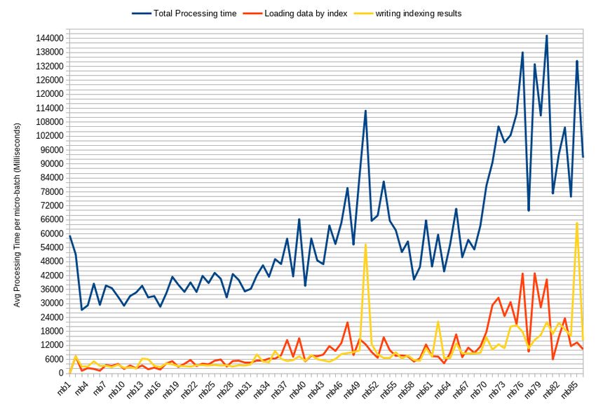
semantics properties, expressed in terms of either RDF Schema and/or OWL,
and aims at inferring the implicit triples that can be derived from D by using
properties in S. Data saturation is crucial in order to ensure that RDF process-
ing and querying actually work on the complete informative content of an RDF
database, without ignoring implicit information. To deal with the problem of sat-
urating massive RDF datasets, a few approaches exploiting big data paradigms
(namely Map-Reduce [10]) and platforms, notably Hadoop and Spark (see e.g.,
[19, 7]), have already been proposed. In [19] Urbani et al. described the WebPIE
system and showed how massive RDF data can be saturated by leveraging on
the Map-Reduce paradigm over Hadoop. In [7] Gu et al. presented the Cichlid
system and showed how to speed up saturation by using Spark and its underlying
Resilient Distributed Datasets (RDDs) abstraction. In [14, 15] authors proposed
a parallel reasoning method based on P2P self-organizing networks, while in [23]
authors propose a parallel approach for RDF reasoning based on MPI. These
approaches, however, assume that RDF datasets are fully available prior to the
saturation, and as such, are not instrumented to saturate RDF data produced
continuously in streams. Indeed, when RDF data are produced in streams, such
systems must re-process the whole data collection in order to obtain triples en-
tailed by the newly received ones. This is due to the fact that both initial and
already obtained triples (by means of past saturation) can entail new triples un-
der the presence of newly received instance/schema triples. A number of works
have addressed the problem of incremental saturation [3, 21, 13, 24], but these
approaches, being mostly centralised, do not ensure scalable, distributed, and
robust RDF streaming saturation.

    To overcome these limitations, in this work we present the first distributed
technique for saturating streams of large RDF data, by relying on a Spark clus-
ter, hence ensuring scalability and robustness. We rely on RDF Schema as a
language to define property triples, since, despite its simplicity, RDF Schema is
rich enough to make the efficient saturation of streaming large RDF data far
from being trivial. The main challenge is to quickly process fresh data, that
must be joined with past met data, whose volume can soon become particularly
high in the presence of massive streams. To this end, unlike existing solutions
[19, 7] for large-scale RDF saturation, upon the arrival of new RDF statements
(both schema and instance triples) our solution finely identifies the subset of the
existing (and already saturated) RDF dataset that needs to be considered. This
is obtained by relying on an indexing technique we devise for our approach.

    The rest of this work is organized as follows. Section 2 presents preliminaries
about RDF saturation and Spark streaming, while Section 3 describes the state-
of-the art concerning large-scale RDF saturation using Spark. Section 4 presents
an overview of our technique by means of examples, while Section 5 describes the
algorithms. Section 6 is dedicated to performance evaluation of our approach.
Sections 7 and 8, respectively, discuss related works and future perspectives.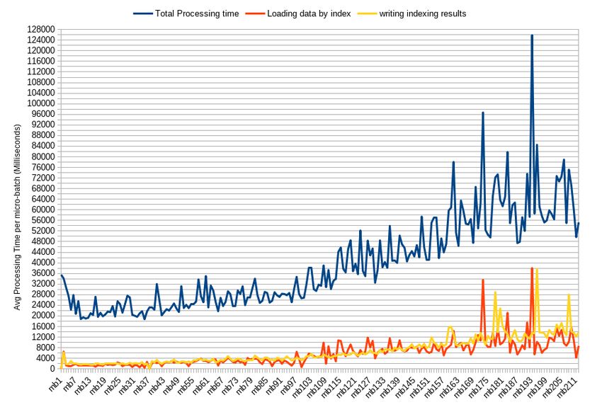
2     Preliminaries
2.1    RDF and Semantic Data Reasoning
An RDF dataset is a set of triples of the form s p o. s is an IRI1 or a blank node
that represents the subject. IRI stands for Internationalized Resource Identifier,
and is used in the semantic web to identify resources. p is an IRI that represents
the predicate, and o is an IRI, blank node or a literal, and it stands for the
object. Blank nodes, denoted as :bi , are used to represent unknown resources
(IRIs or literals). RDF Schema (or RDFS for short) provides the vocabulary
for specifying the following relationships between classes and properties, relying
on a simplified notation borrowed from [6]: subclass relationship ≺ sc : the triple
c1 ≺ sc c2 specifies that c1 is a subclass of c2 ; subproperty relationship ≺ sp : the
triple p1 ≺ sp p2 specifies that p1 is a sub-property of p2 ; property domain ←- d :
the triple p ←- d x specifies that the property p has as a domain x; and property
range ,→ r : the triple p ,→ r z specifies that the property p has as a range z.
For the sake of readability, in what follows we use simple strings instead of IRIs
to denote predicates, subjects and objects in triples. Also, we abbreviate the
rdf:type predicate with the τ symbol.
Example 1. Figure 2 illustrates a set of RDF instance triples that we use as a
running example, together with the equivalent graph representation. The graph
describes the resource doi1 that belongs to an unknown class, whose title is
“Complexity of Answering Queries Using Materialized Views”, whose author
is “Serge Abiteboul” and having an unknown contact author. This paper is in
the proceedings of an unknown resource whose name is “PODS0 98”. Lastly, the
IRI edbt2013 is a conference and hasName, the property associating names to
resources, is created by “John Doe”.
    Figure 1 lists schema triples. For example, it specifies that the class posterCP
is a subclass of ConfP, that the property hasContactA is a sub-property of
hasAuthor. It also specifies that the property hasAuthor has as domain paper
and as range a literal.

             S = { posterCP ≺ sc confP,       :b0 ≺ sc confP,
             confP ≺ sc paper,               hasTitle ←- d confP,
             hasTitle ,→ r rdfs:Literal,     hasAuthor ←- d paper,
             hasAuthor ,→ r rdfs:Literal,    hasContractA ≺ sp hasAuthor,
             inProceesingOf ←- d confP,      inProceesingOf ,→ r conference,
             hasName ←- d conference,        hasName ,→ r rdfs:Literal,
             createdBy ,→ r rdfs:Literal }

                     Fig. 1: Instance and schema RDF triples.

1
    An IRI (Internationalized Resource Identifier ) is just a URI exploiting Unicode in
    place of US Ascii as the character set.
G = { doi1 τ :b0 , doi1 hasTitle “CAQU MV”,
doi1 hasAuthor “SA”, doi1 hasContactA :b1 ,
doi1 inProceedingsOf :b2 , :b2 hasName “PODS0 98”,
hasName createdBy “John Doe”, “edbt2013” τ Conference }
createdBy
:b0 hasName “John Doe”
τ
itle
hasT “CAQU MV”
hasAuthor τ
G = doi1 “SA” “edbt2013” Conference
has
inP ContactA
roc :b1
eed
ing
sO
f hasName
:b2 “PODS0 98”
Fig. 2: RDF graph representation of a conference paper.
As in other works (e.g., [6, 7, 19]) we focus on the core rules of RDFS, the
extension to other rules being trivial. In particular, we consider here rules 2, 3,
5, 7, 9, and 11 among the 13 RDFS rules illustrated in Table 1.
The realm of the semantic web embraces the Open World Assumption: facts
(triples) that are not explicitly stated may hold given a set of RDFS triples
expressing constraints. These are usually called implicit triples, and, in our work,
we consider the problem of RDF saturation, i.e., given a set of RDFS rules,
inferring all possible implicit triples by means of these rules applied on explicit
triples, or, recursively, on implicit triples. For example, rule rdfs2 in Table 1
states that, if a property p has a domain x, given a triple s p o, we can infer that
s is of type x. Since rdfs9 specifies that, if s is of type x and x is a subclass of
y, then we can infer that s is of type y.
Table 1: RDFS rules.
Rule Condition Consequence level
rdfs1 spo :b τ rdfs:Literal -
rdfs2 p ←- d x, s p o sτ x instance-level
rdfs3 p ,→ r x, s p o oτ x instance-level
rdfs4 spo s/o τ rdfs:Resource -
rdfs5 p ≺ sp q, q ≺ sp r p ≺ sp r schema-level
rdfs6 p τ rdf:Property p ≺ sp p -
rdfs7 s p o, p ≺ sp q sqo instance-level
rdfs8 s τ rdfs:Class s ≺ sc rdfs:Resource -
rdfs9 s τ x, x ≺ sc y sτ y instance-level
rdfs10 s τ rdfs:Class s ≺ sc s -
rdfs11 x ≺ sc y, y ≺ sc z x ≺ sc z schema-level
rdfs12 p τ rdfs:ContainerMembershipProperty p ≺ sp rdfs:member -
rdfs13 o τ rdfs:Datatype o ≺ sc rdfs:Literal -In the remaining part of the paper, we will use the following notation to
indicate derivations/inference of triples. A derivation tree is defined as follows.
T := t | {T | T } − rdfsX → t
where the rule number X ranges over {2, 3, 5, 7, 9, 11}. A derivation tree can be
empty, hence consisting of a given triple t, or can be of the form {T 1 | T 2} −
rdfsX → t, meaning that the tree derives t, by means of rule rdfsX whose
premises are (matched to) the two triples given by T1 and T2, respectively. So,
for instance we can have the following derivation tree T1 for the for G and S
previously introduced:
{hasT itle ←- d conf P | doi1 hasTitle “CAQU MV”} − rdfs2 → doi1 τ conf P
Moreover, we can have the following derivation T2 relying on T1: {T 1 | conf P ≺
sc paper} − rdfs9 → doi1 τ paper.
In the following, given a set of instance RDF triples D and a set of schema
triples S, we say that T is over D and S if the derivation tree uses triples in D
and S as leaves. Moreover, we define the saturation of D over S as D extended
with all the possible instance triples obtained by means of derivation (below,
derivation trees are assumed to be over D and S):
DS∗ = D ∪ {t | ∃{T 1 | T 2} − rdfsX → t with X ∈ {2, 3, 7, 9}}
Notice above that, say, T2 can be a derivation tree totally over S, recursively
applying rule 5 (or rule 11) thus deriving a triple in S ∗ , below defined.
S ∗ = S ∪ {t | ∃{T 1 | T 2} − rdfsX → t with X ∈ {5, 11}}
Above, in the S ∗ definition, please note that since X ∈ {5, 11} the whole deriva-
tion tree consists of subsequent applications of rule rule 5 (or rule 11).
2.2 Spark and Spark Streaming
Spark [25] is a widely used in-memory distributed cluster computing framework.
It provides the means for specifying DAG-based data flows using operators like
map, reduceByKey, join, filter, etc. over data collections represented by means of
Resilient Distributed Datasets (RDDs). For our purposes, we use the streaming
capabilities of Spark whereby data comes into micro-batches that needs to be
processed within a time-interval (also referred to as a window).
3 Saturating Large RDF Graphs Using Spark
We already briefly discussed in the introduction the Cichlid system [7], which
represents the state of the art of RDF saturation, and WebPIE [19]. As in our
case, these systems focus on rules 2, 3, 5, 7, 9, and 11, illustrated in Table 1.While the outcome of the saturation operation is orthogonal to the order
in which the rules are applied, the time and resources consumed by such an
operation are not. Because of this, the authors of Cichlid (and WebPIE before
them) identified a number of optimisations that influence the rule application
order with the view to increasing the efficiency of the saturation. In what follows,
we discuss the main ones.
1. RDF Schema is to be saturated first. The size of the RDF schema2 in an
RDF graph is usually small, even when saturated. It is usually orders of
magnitudes smaller than the size of the remaining instance triples. This
suggests that the schema of the RDF graph is to be saturated first. By
saturating the schema of an RDF graph we mean applying rules that produce
triple that describes the vocabulary used in an RDF graph. Furthermore,
because the size of the schema is small, schema saturation can be done in
centralized fashion. In this respect, the RDFS rules presented in Table 1 can
be categorised into two disjoint categories: schema-level and instance-level
RDFS rules. Schema-level RDFS rules (rdfs5 and rdfs7 ) designate the rules
that produce triples describing the vocabulary (classes, properties, and their
relationships). Instance-level triples, on the other hand, specifies resource
instances of the classes in the RDF vocabularies and their relationships.
Each rule is made up of two premises and one conclusion, each of which
is an RDF triple. While premises of schema-level rules are schema triples,
premises of instance-level rules are a schema triple and an instance triple.
Also, instance-level rules entail an RDF instance triple, while schema-level
rules entail an RDF schema triple.
2. Dependencies between rules. When determining the rule execution order, the
dependencies among rules must be taken into account too. In particular, a
rule Ri precedes a rule Rj if the conclusion of Ri is used as a premise for rule
Rj . For example rdfs7 has a conclusion that is used as a premise for rules
rdfs2 and rdfs3. Therefore, rdfs7 should be applied before rdfs2 and rdfs3.
By taking (1) and (2) into consideration, the authors of Cichlid established
the orders of applications of rules illustrated in Figure 3. To illustrate how rules
are implemented in Spark, we will use a concrete example considering rdfs9,
which can be expressed as follows. If a resource s is of type x, i.e. s τ x, and x
is a sub-class of y, i.e. x ≺ sc y, then s is also an instance of y, i.e. s τ y. Note
that, as the output of rdfs2 and rdfs3 are instance triples with predicate τ , these
rules are executed in Cichlid before executing rdfs9 (see [7] for more details). In
our approach we will rely on the same ordering for streaming saturation.
To implement rdfs9 in Spark, Cichlid uses the f ilter, map, and collect op-
erators in Algorithm 1. The algorithm first retrieves over all the partitions the
RDFS schema, the classes and their corresponding sub-classes in the schema,
by means of the filter transformation and the collect action (this last one is
2
By Schema, we mean the RDF triples that describe the vocabulary of an RDF graph,
i.e., classes, properties and their constraints.rdfs9
subClassOf.
instance-level
rdfs2 rdfs3 rdfs11
domain. range. subClassOf.
instance-level instance-level transitivity
rdfs7 rdfs5
subPropertyOf. subPropertyOf.
instance-level transitivity
Fig. 3: The optimized execution RDFS rules order. Dashed ellipses show the schema-
level entailment, while the solid ellipses are for the Instance-level entailment. The white
colour ellipse has no dependency prerequisite with other RDFS. The lighter ellipses come
first.
Algorithm 1 Optimized Parallel reasoning of RDFS rdfs9
1: Input: input triple set named triples
2: Output: reasoning results named results
3: Begin
4: val schema = sc.textFile(“hdfs://schema-path”)
5: val subClassOf = schema
6: .filter (t ⇒ t. 2.contains(“rdf s : subClassOf 00 ))
7: .map(t ⇒ (t. 1, t. 3)).collect
8: val bc = sc.broadcast(subClassOf.toMap)
9: val triples = sc.textFile(“hdfs://instance-path”)
10: val results = triples.filter(t ⇒ bc.value.contains(t. 3))
11: .map(t ⇒ (t. 1, τ , bc.value(t. 3))
12: End
needed in order to collect on the master/driver machine the total filtered in-
formation). This information is then broad-casted3 (i.e., locally cached in each
machine in the cluster) as pairs (e.g., x → y), thereby avoiding the cost of
shipping this information every time it is needed. It first retrieves the RDFS
schema (line 4), the classes and their corresponding sub-classes (lines 5-7),
and the obtained information is then broad-casted (line 8). Therefore, for
each broad-casted pair of subclass and superclass, the instances of the sub-
class are retrieved (line 9), and new triples are derived stating that such in-
stances are also instances of the broad-casted super-class, by means of the
map transformation (line 10-11). Spark provides other operators, which are
used for implementing other rules, such as distinct, partitionBy, persist, union,
mapP artitions, mapP artitionsW ithIndex, etc.
Notice that as the saturation process may derive triples that are already
asserted or have been derived in previous steps of the saturation operation,
Cichlid [7] eliminates the duplicated triples from the derived ones, in order to
improve efficiency.
3
Broadcast operation can be used in Spark to cache a copy of data on every node of
a cluster. This helps in avoiding the cost of shipping this information every-time it
is used by the nodes.4 Our Contribution: Streaming RDF Saturation
Our goal is to support the saturation of RDF streams by leveraging on Spark
stream processing capabilities. Using Spark, an RDF stream is discretized into
a series of timestamped micro-batches that come (and are, therefore, processed)
at different time intervals. In our work, we assume that a micro-batch contains
a set of instance RDF triples, but may also contain schema (i.e., RDFS) triples.
Consider, for example, an RDF stream composed of the following series of
micro-batches [mbi , . . . , mbn ], where i > 0. A first approach for saturating such a
stream using a batch-oriented solution would proceed as follows: when a micro-
batch mbi arrives, it unions mbi with the previous instance dataset (including
triples obtained by previous saturation) and then the resulting dataset is totally
re-saturated.
On the contrary, our approach allows for RDF saturation in a streaming
fashion, by sensibly limiting the amount of data re-processing upon the arrival
of a new micro-batch. To this end we have devised the following optimization
techniques:
1. Rule pruning for schema saturation. Given a new micro-batch mbi , we filter
all the schema triples contained in it. Note that in the general case it is not
likely that these new schema triples trigger all the saturation rules, i.e. it is
not the case that the new micro-batch includes all kinds of RDFS triples at
once - i.e. subPropertyOf, domain, range, and subClassOf. So for saturating
the schema at the level of the new micro-batch we first filter new schema
triples, and then obtain the set of new schema triples NST = Saturation(new
received schema ∪ past schema) - past schema. The Saturation operation is
local and only triggers rules that do need to be applied, in the right order. All
possible cases are indicated in Table 2, and Saturation selects one line of this
table, depending on the kind of schema predicates met in the new schema
triples. This avoids triggering useless rules. Once saturation for mbi schema
triples is done in this optimized fashion, obtained triples are merged with the
existing RDFS schema for a second-pass of global schema saturation, taking
into account triples deriving from both mbi and the pre-existing schema.
2. Efficiently saturate existing instance triples by leveraging our incremental
indexing scheme. Given the new schema triples that are provided by the
micro-batch mbi or inferred in (1), we need to scan existing instances triples
to identify those that if combined with the new schema triples will trigger
RDFS rules in Table 1. This operation can be costly as it involves examining
all the instance triples that have been provided and inferred micro-batches
received before mbi . To alleviate this problem, we have devised an incre-
mental indexing technique that allows for the fast retrieval of the instance
triples that are likely will trigger the RDFS rules given some schema triples.
The technique we developed index instance triples based on their predicate
and object, and, as we will show later, allow to greatly reduce the data pro-
cessing effort for the saturation under the new schema. Once retrieved, such
instances triples are used together with the new schema triples to generateTable 2: The 1 and 0 indicate for the availability of that particular schema
rules in mbi . X → Y means: The output of rule X used as an input of rule
Y.
subPropertyOf domain range subClassOf Saturation order
1 1 1 1 1 R7 → (R2, R3) → R9
2 1 1 1 0 R7 → (R2, R3)
3 1 1 0 1 R7 → R2 → R9
4 1 1 0 0 R7 → R2
5 1 0 1 1 R7 → R3 → R9
6 1 0 1 0 R7 → R3
7 1 0 0 1 R7, R9
8 1 0 0 0 R7
9 0 1 1 1 (R2,R3) → R9
10 0 1 1 0 R2, R3
11 0 1 0 1 R2 → R9
12 0 1 0 0 R2
13 0 0 1 1 R3 → R9
14 0 0 1 0 R3
15 0 0 0 1 R9
16 0 0 0 0 -
new instance triples. Notice here that we cannot infer new schema triple.
This is because the rules for inferring new schema triples require two schema
triples as a premise (see Table 1).
3. Saturate new instance triples. As well as those that are inferred in (2) need to
be examined as they may be used to infer new instance triples. Specifically,
each of those triples is examined to identify the RDFS rule(s) to be triggered.
Once identified such rules are activated to infer instance triples. The instance
triples in mbi as well as those inferred in (2) and (3) are stored and indexed
using the method that we will detail next.
We will now turn our attention to our indexing scheme, mentioned above.
For a micro-batch mbi received at time-stamp t we create an HDFS directory
named as t, in which we store other indexing information related to mbi , as
follows. The instance triples that are asserted in mbi , as well as those that are
inferred (see (2) and (3) above), are stored into two t separate sub-directories,
which we name o and p.
The instances triples in mbi that provide information about the type of a
resource, i.e., having as predicate rdf:type, are stored in the o directory. Such
triples are grouped based on their object and they are stored in files within the
o directory of the micro-batch mbi . Specifically, instance triples with the same
object are stored in the same file. Additionally, our indexing scheme utilizes
an associative hash-table stored in a cached RDD in main memory, associating
each encountered object with the list of HDFS addresses corresponding to files
in the o directories, which include at least one triple with that object. Noticethat triples with the rdf:type predicate are used in the premises of rdfs9. Given
a schema triple of the form y ≺ sc z, our indexing approach allows for the fast
retrieval of the files in the o directories of the micro-batches that have as an
object the resource y, and therefore can be used to trigger rdfs9.
The remaining instance triples in mbi , i.e., those that do not have rdf:type
as a predicate, are grouped based on their predicate, and stored within files
under the p directory. Additionally, an associative hash-table stored in an RDD
persisted in main memory, associating each encountered property with the list
of HDFS addresses corresponding to files in the p directories including at least
one triple with that property is created and maintained. By means of this kind
of indexing, we can optimize application of rules rdfs2, rdfs3 and rdfs7 to infer
new instance triples as we can inspect the previously described hash-table in
order to retrieve only files containing triples with properties needed by these 3
rules.
To illustrate, consider for example that a new micro-batch mbi arrives at a
given time instant t, and that it contains the schema triple tsc : s1 ≺ sc s2 . Such
schema triple can contribute to the inference of new schema triples (i.e., by means
of rdfs11 ) as well as new instance triples by means of rdfs9. Since the indexation
mechanism we elaborated is sought for the inference of instance triple, let us
focus on rdfs9. To identify the instance triples that can be utilized together
with the schema triple tsc , we need to examine existing instance triples. Our
indexing mechanism allows us to sensibly restrict the set of triples that need to
be examined, as the hash-table indexing the files under the o directories enables
the fast recovering of files containing triples with s1 as an object resource, and
that can be combined with the schema triple tsc to trigger rdfs9. The indexing on
files in p directories are operated in a similar manner in order to efficiently recover
files containing instance triples with a given property so as to use included triples
to trigger rdfs2/3/7, under the arrival of a correspondent schema triple in the
stream.
To illustrate our approach more in detail let’s consider the following example.
Example 2. We assume that we have the initial schema S of Figure 1 and that
we saturate it by obtaining S0 as indicated below.
S0 = S ∪ { hasContactA ,→ r rdfs:Literal, :b0 ≺ sc paper }
This operation is fast and centralized, as the initial schema is always relatively
small in size. Our approach then proceeds according to the following steps.
1. The saturated schema S0 is broad-casted to each task, so that it can access
S0 with no further network communication.
2. Then available micro-batches are processed. For the sake of simplicity we
make here the, unnatural, assumption that each micro-batch consists of only
one triple. The stream of micro-batches is in Table 3.
3. The first received micro-batch triggers rdfs9 so that we have the derivation
of two new triples:
{doi1 τ : b0 | : b0 ≺sc conf P } − rdfs9 → doi1 τ conf P
{doi1 τ : b0 | : b0 ≺sc paper} − rdfs9 → doi1 τ paperTable 3: Instance triples
mb Subject Predicate Object
1 doi1 τ :b0
2 doi1 hasTitle “CAQU MV”
3 doi1 hasAuthor “SA”
4 doi1 hasContactA :b1
5 doi1 inProceedingsOf :b2
6 :b2 hasName “PODS0 98”
The received triple plus the two derived ones are then stored according to
our indexing strategy. As already said, triples are grouped by their objects
when having rdf:type property, so as to obtain the following file assignment,
knowing that t1 is the time stamp for the current micro-batch:
doi1 τ confP ⇒ o/t1 /f ile1 ,
doi1 τ paper ⇒ o/t1 /f ile2 ,
doi1 τ :b0 ⇒ o/t1 /f ile3
4. The processing goes on by deriving new instance triples for the micro-batches
from 2 to 6, as indicated in the Table 4, which also indicates how instance
triples are stored/indexed.
Table 4: Saturated streaming triples
mbi Received triple(s) Schema-triple Entails(E.) & Received(R.) stored path
1 doi1 τ :b0 :b0 ≺ sc confP, E. doi1 τ confP, o/t1 /file1 ,
:b0 ≺ sc paper E. doi1 τ paper, o/t1 /file2 ,
R. doi1 τ :b0 o/t1 /file3
2 doi1 hasTitle “CAQU MV” hasTitle ←- d confP E. doi1 τ paper, o/t2 /file1 ,
R. doi1 hasTitle “CAQU MV” p/t2 /file1
3 doi1 hasAuthor “SA” hasAuthor ←- d paper E. doi1 τ paper, o/t3 /file1 ,
R. doi1 hasAuthor p/t3 /file1
“SA”
4 doi1 hasContactA :b1 no inference R. doi1 hasCon- p/t4 /file1
tactA :b1
5 doi1 inProceedingOf :b2 inProceesingOf ←- d confP, E. doi1 τ confP, o/t5 /file1 ,
inProceesingOf ,→ r conference E. :b2 τ conference, o/t5 /file2 ,
R. doi1 inProceedingOf :b2 p/t5 /file1
0
6 :b2 hasName “PODS 98” hasName ←- d conference E. :b2 τ conference, o/t6 /file1 ,
R. :b2 hasName “PODS0 98” p/t6 /file1
Now assume that in micro-batch 7 we have the followed RDF schema triples:NST = { paper ≺ sc publication, hasContactA ≺ sp hasAuthor
posterCP ≺ sc publication, confP ≺ sc publication,
:b0 ≺ sc publication, hasContactA ←- d paper }
Fig. 4: N ew received and inferred S chema T riples (NST )
paper ≺ sp publication,
hasContractA ≺ sp hasAuthor
So we have now three steps: i) infer the new schema triples plus filtering
out already present triples, ii) broadcast these schema triples minus the already
exist/broadcast schema triples (Figure 4), to enable tasks to locally access them,
iii) re-processing previously met/inferred instance triples by taking into consid-
eration the new schema. Consider for instance {hasContactA ≺ sp hasAuthor}
as new schema triple. This schema triple triggers rdfs7. Therefore, our indexing
tells us that only file p/t4 /file1 (Table 4, line 4) needs to be loaded to infer new
triples, that, of course, will be in turn stored according to our indexing strategy.
As we will see in our experimental analysis, the pruning of loaded files en-
sured by our indexing will entail fast incremental saturation. Also, note that
our approach tends to create a non-negligible number of files, but fortunately
without compromising efficiency thanks to distribution.
5 Streaming Saturation Algorithm
The overall streaming saturation algorithm is shown in Algorithm 2, and com-
mented hereafter.
Given a micro-batch mbi , we first perform schema saturation if mbi contains
schema triples (lines 12, 13 ). The related instance triples are retrived based on
mbNST (line 14 ). Given newly inferred schema triples, instance triples are reterived
and examined to identify cases where new instance triples may be inferred (line
15 ). The obtained schema triples (i.e., mbNST ) are added and broad-casted within
the intial schema RDD (line 17, 18 ). The inferred triples, if any, are merged with
instance triples of mbi (i.e., mbins ) and the saturation is applied to them. In the
next step, the received and inferred instance triples are combined and obtained
duplicates, if any, are removed (line 22 ). In the last step, the instance triples
from the previous step are saved and indexed using our method (line 24-25 ).
Otherwise by receiving an RDFS free mbi , the applied saturation process on
the mbi (line 21-25 ) is same as Cichlid. The results then will send to Indexing
algorithm (Algorithm 3) to store on HDFS at the intended paths but also collect
the object/predicate of triples and their paths for indexing variable. We rather
focus here on the algorithm for indexing, which is central to our contribution.
Central to the efficiency of the solution presented in the previous section is the
technique that we elaborated for incrementally indexing the new instance triples
that are asserted or inferred given a new micro-batch.Algorithm 2 Overall algorithm for saturating RDF stream.
1: Input: MB ← [mb1 , · · · , mbn ] // a stream of micro-batches.
2: Output: Schemas ← [Sch1 , · · · , Schn ] // Schi represents the schema triples obtained as a result
of saturating the micro-batches MB = [mb1 , · · · mbi ].
3: Output: Datasets ← [DS1 , · · · , DSn ] // DSi represents the instance triples obtained as a result of
saturating the micro-batches MB = [mb1 , · · · mbi ].
4: Output: IndexInformations ← [oIndex, pIndex] // oIndex and pIndex keeps object- and predicate-
based information respectively.
5: Dins ← ∅ // Initialize a dataset for instance triples
6: Dsc ← ∅ // Initialize a dataset for schema triples
7: br ← if Dsc exist then TransitiveClosure and broadcast them
8: do {
9: (mbsch , mbins ) ← SeparatingTriples(mbi ) // Separate schema from instance triples in mb
10: if (mbsch exist then) {
11: // i) Retrieve the already saturated instance triples and re-saturate them based on combi-
nation of received and existing RDFS triples
12: mb0sch ← (TransitiveClosure (mbsch ∪ Dsc )) - Dsc
13: mbNST ← broadcast(mb0sch ) // Just updated parts
14: D0ins ← Retrieve saturated triples using Indexing variable based on mbNST
15: mb0i ← Saturate(D0ins , mbNST )
16: // Combine received and existing RDFS triples and re-broadcast them
17: Dsc ← mbNST ∪ Dsc
18: br ← broadcast(Dsc ) // The total so far schema received.
19: }
20: // Saturate the received instance triples with total RDFS triples
21: mbimp ← Saturate(mbins ∪ mb0i , br)
22: mb00i ← (mbins ∪ mbi 0 ∪ mbimp ).distinct
23: // The following two lines are handled by Indexing Algorithm
24: Save mb00i in the HDFS
25: [oIndex, pIndex]∪ ← indexing(mb00i )
26: } while(is there an incoming micro-batch mb?)
27: End
As mentioned in the previous section, indexed instance triples are classified
into two disjoint categories: object- or predicate-based triples. Specifically, a triple
is considered an object-based if its predicate is rdf:type. Triples of this kind are
used as a premise to rdfs9 (see Table 1). On the other hand, a triple is considered
to be predicate-based if its predicate is different from rdf:type. Triples of this
kind are used as premise for rules rdfs2, rdfs3 and rdfs7 (see Table 1).
Labeling a new instance triple as object-based or predicate-based is not suf-
ficient. To speed up the retrieval of the triples that are relevant for activat-
ing a given RDFS rule, object- and predicate-based triples are grouped in files
based on their object and predicate. This allows for triples having a given pred-
icate/object to be located in only one file inside the directory associated with
a micro-batch. More specifically, Algorithm 3 details how the indexation oper-
ation is performed. It takes as input new instance triples that are asserted or
inferred given the last micro-batch mb0 . It filters the instances triples to create
two RDDs. The first RDD is used for storing object-based triples (line 9-11).
Since the predicate of object-based triples is rdf:type, we only store subject
and object of object-based triples. The second RDD is used for predicate-based
triples (line 13-15). Notice that the triples of the two RDDs are grouped based
on their object and predicate, respectively, by utilizing RDD partitioning. The
Spark method partitionBy() takes as an argument the number of partitions to
be created. In the case of the RDD used for storing object-based triples, we useAlgorithm 3 Incremental RDFS Indexing Algorithm
1: // mb0i is indicated as instance and implicit triples from received mb0i
2: Input: Saturated mb0i
3: // The information of mb0i keeps as two RDDs in memory.
4: Output: oIndexingRDD, pIndexingRDD
5: Begin
6: // Get a f ixed timestamp to save the mb0i triples.
7: val fts = System.currentTimeMillis.toString
8: // The mb0i triples partitions by their object where their predicate is rdf:type.
9: val oPartition = mb0i .filter( . 2.contains(“rdf-syntax-ns#type”)).
10: map(t ⇒ (t. 3, t. 1)).partitionBy(number of different object).
11: mapPartitions( .map(t ⇒ (t. 2, t. 1)))
12: // The mbi 0 triples partitions by their predicate where their predicate is NOT rdf:type.
13: val pPartition = mb0i .filter(! . 2.contains(“rdf-syntax-ns#type”)).
14: map(t ⇒ (t. 2, t)).partitionBy(number of different predicate).
15: mapPartitions( .map( . 2))
16: // The oPartitions and pPartitions store on HDFS at fixed timestamp under o and p sub-
directory paths respectively.
17: oPartition.saveAsTextFile(outputPath + “o/” + fts + “/data/”)
18: pPartition.saveAsTextFile(outputPath + “p/” + fts + “/data/”)
19: // oIndexingRDD is a HashTable which keeps the object of instance triple as key and their
physical paths as value.
20: oIndexingRDD += ∪ oPartition.mapPartitionsWithIndex((index,iterator ) ⇒{
21: iterator.map(t ⇒ (t. 2, fts + “-” + index + “ ”)) }).mapPartitions(
22: .map(t ⇒ (t,1))).reduceByKey( + ).mapPartitions( .map( . 1))
23: // pIndexingRDD is a HashTable which keeps the predicate of instance triple as key and
their physical paths as value.
24: pIndexingRDD += ∪ pPartition.mapPartitionsWithIndex((index,iterator ) ⇒{
25: iterator.map(t ⇒ (t. 2, fts + “-” + index + “ ”)) }).mapPartitions(
26: .map(t ⇒ (t,1))).reduceByKey( + ).mapPartitions( .map( . 1))
27: return oIndexingRDD & pIndexingRDD
28: End
the number of different objects that appear in the triples as an argument. In the
case of the RDD used for storing predicate-based triples, we use the number of
different predicates that appear in the triples. It is worth mentioning here that
we could have used the method sortBy() provided by Spark for RDDs instead
of partitionBy(). However, sortBy() is computationally more expensive as it
requires a local sort.
Besides grouping the RDDs containing the triples, the algorithm creates
two auxiliary lightweight hash structures to keep track of the partitions that
store triples with a given object (line 20-22) and predicate (line 24-26), respec-
tively. Such memory-based hash structures act as indexes. They are lightweight
memory-based structures that are utilized during the saturation to quickly iden-
tify partitions that contain a given object and predicate, respectively. Note that
all the steps of the algorithm, with the exception of the first one (line 7) are
processed in a parallel manner.
Soundness and completeness. We deal now with the proof of soundness
and completeness of our approach.
We need the following lemma, which is at the basis of soundness and com-
pleteness of our system as well as of WebPIE [19] and Cichlid [7], and reflects
rule ordering expressed in Figure 3. To illustrate the lemma, assume we have
D = {s τ c1} while the schema includes four triples of the form ci ≺ sc ci+1 , fori = 1 . . . 4. Over D and S we can have the tree T1 corresponding to:
{c1 ≺ sc c2 | c2 ≺ sc c3 } − rdfs11 → c1 ≺ sc c3
A more complex tree is T2 defined in terms of T1:
{s τ c1 | T 1} − rdfs9 → s τ c3
Imagine now we have T3 defined as
{c3 ≺ sc c4 | c4 ≺ sc c5 } − rdfs11 → c3 ≺ sc c5
We can go on by composing our derivation trees, obtaining T4:
{T 2 | T 3} − rdfs9 → s τ c5
Note that the above tree T4 includes two applications of rdfs9. At the same time
we can have the tree T5
{T 1 | T 3} − rdfs11 → c1 ≺ sc c5
enabling us to have the tree T40 which is equivalent to T4, having only one
application of rule 9, and consisting of
{s τ c1 | T 5} − rdfs9 → s τ c3
As shown by this example, and as proved by the following lemma, repeated
applications of instance rules {2, 3, 7, 9} can be collapsed into only one, provided
that this rule is then applied to an instance triple and to a schema triple in S ∗ ,
obtained by repeated applications of schema rules 5 and 11. This also proves
that it is sound to first saturate the schema S and then applying instance rules
{2, 3, 7, 9} (each one at most once) over schema rules in S ∗ .
Lemma 1. Given an RDF data set D of instance triples and a set S of RDFS
triples, for any derivation tree T over D and S, deriving t ∈ DS∗ , there exists
an equivalent T0 deriving t, such that each of the instance rules {2, 3, 7, 9} are
used at most once, with rule 7 applied before either rule 2 or 3, which in turn is
eventually applied before 9 in T0 . Moreover, each of these four rules is applied
to a S ∗ triple.
Proof. To prove the above lemma, we examine the dependencies between
the rules {2, 3, 5, 7, 9, 11}. A rule r depends on a rule r0 where possibly r and r0
are the same rule, if the activation of r0 produces a triple that can be used as
a premise for the activation of r. This examination of rule dependencies reveals
that:
– Rule 5 depends on itself only.
– Rule 11 depends on itself only..
– Rule 7 depends on rule 5: rule 7 uses as a premise triples of the form p ≺ sp q,
which are produced by the activation of rule 5.– Rules 2 and 3 depend on rule 7: both rules 2 and 3 uses as a premise triples
of the form spo, which are given in prior and produced by rule 7.
– Rule 9 depends on rules 2, 3 and all given triples in prior with τ as a pred-
icate: both rules produce triples of the form p τ x, a premise for activating
rule 9. It also depends on rule 5.
Rule 9
Rule 2 Rule 3
Rule 7
Rule 5 Rule 11
Rule dependency
Fig. 5: RDFS rule dependencies.
Figure 5 depicts the obtained rule dependency graph. With the exception of
rule 5 and 11, the graph is acyclic, meaning that the saturation can be performed
in a single pass. Furthermore, the dependency graph shows that in order for the
saturation to be made in a single pass schema rules 5 and 11 needs to be first
(transitively) applied to saturate the schema, followed by the instance rules. Rule
7 is the first instance rule to be executed, followed by the instance rules 2 and
3 (which can be applied simultaneously or in any order), before applying at the
end rule 9. That said, we need to prove now that for for an arbitrary T there is
exist an equivalent T0 as described in the lemma. This follows from the fact that
if (*) T contains more than one rule rdfsX with X ∈ {2, 3, 7, 9}, then it must be
because of subsequent applications of rule 9 (resp. rule 7) each one applied to
a schema triple eventually derived by rule 11 (resp. rule 5), exactly as depicted
by the example just before the lemma. As shown by the example, this chain
of rule 9 (resp. rule 7) applications can be contracted so as to obtain a unique
application of rule 9 (resp. rule 7) applied to as schema triple in S ∗ , obtainedby subsequent applications of rule 11 (resp. rule 9). So in case (*) holds, the
just described rewriting for chains of rule 9 (resp. rule 7) can be applied to T in
order to obtain T0
t
u
Given the above lemma, we can now present the theorem stating the sound-
ness of our approach.
Theorem 1. Given a set of instance triples D and schema triples S, assume
the two sets are partitioned in n micro-batches mbi = Di ∪ Si with i = 1 . . . n,
we have that there exists a derivation tree {T 1 | T 2} − rdfsX → t over D and
S, with t ∈ DS∗ , if and only if there exists j ∈ {1, . . . , n} such t is derived by
our system when mbj is processed, after having processed micro-batches mbh with
h = 1 . . . j − 1.
Proof. The ’if’ direction (soundness) is the easiest direction. We prove this case
by induction on j. In case one triple t is derived by our system when processing
the micro-batch mb1 , then we can see that in Algorithm 2, this triple is obtained
by a derivation tree calculated by Saturate(), and including at the leaves instance
triple in D1 and schema triple in S1 ∗ . As D1 ⊆ D and S1 ∗ ⊆ S ∗ , we have that his
derivation tree can derive t also from D and for S. Assume now t is derived by
our system when processing the micro-batch mbj with j > 1. Triple t is derived
by a derivation tree T possibly using triples t0 derived in mbh with h < j, as
Sj ∗
well as triples in Dj and ( 1 Si ) . By induction we have that for each t0 derived
at step h < j there exists a derivation tree T’over D and S deriving t0 . So to
conclude it is sufficient to observe that if in T we replace leaves corresponding
to triples t0 with the corespondent T 0 then we obtain the desired derivation tree
for t.
Let’s now consider the ’only-if’ direction (completeness). We proceed by a
double induction, first on n, the number of micro-batches, and then on the size of
the derivation tree T deriving t. Assume n = 1, this means that we only process
one micro-batch. By Lemma 1 we have that there exists an equivalent T’ for t,
satisfying the properties stated in the lemma, and hence that can be produced
by our algorithm, as we first saturate the schema and then apply instance rules
in sequence 7-2-9 or 7-3-9, as in T’.
Assume now n > 1. We proceed by induction on the tree derivation T =
{T 1 | T 2} − rdfsX → t. The base case is that both T1 and T2 are simple triples
in D and S respectively. In this case let j be the minimal index ensuring that
both triples have been met in processed micro-batches mbh , with h ≤ j. This j
exists by hypothesis, and we have that either t1 or t2 is in mbj . Assume it is t1,
a schema triple and that t2 has been met in mbs with s < j. Then by means of
our index we recover t2 (line 14) and saturation for the step j in line 21, builds
T to derive the triple t.
Assume now that both T1 and T2 do not consist of a simple triple (the
case only one is a triple is similar). By Lemma 1, we have that there exists an
equivalent T 0 = {T 10 | T 20 } − rdfsY → t such that instance rules are use a
most once (in the order of Figure 3), where each rule uses a schema triple inS ∗ . This 0 0 ∗
Sn means that, w.l.o.g, T2 is a schema triple t2 in S . By hypothesis
(S = 1 Si ) we have that there exists mbh such that t2 is obtained by schema
saturation (which is globally kept in memory) and that there exists mbs in which
t1 is derived and indexed by our algorithm. Now consider j = max(s, h). At
step j our algorithm disposes of both t1 (indexed) and t2 (in the RAM) and can
hence produce {t1 | t2} − rdfsY → t.
The remaining cases are similar. t
u
6 Evaluation
The saturation method we have just presented lends itself, at least in principle,
to outperform state of the art techniques, notably Cichlid, when dealing with
streams of RDF data. This is particularly the case when the information about
the RDF schema is also obtained in a stream-based fashion.
An empirical evaluation is, however, still needed to be able to answer the
following question: Does our method actually outperform in practice the Cichlid
solution for saturating streams of RDF? And if so, to what extent? To answer
this question, we conducted an experimental analysis that we reported on in this
section.
6.1 Datasets
Pre-processing data in stream We used for our experiments three RDF
datasets that are widely used in the semantic web community: DBpedia [2],
LUBM [8], and dblp4 . These datasets are not stream-based datasets, and there-
fore we had to partition them into micro-batches to simulate a setting where
the data is received in a streamed manner. We make in our experiments the
assumption that a substantial part of the data is received initially and that
micro-batches arrive then in a streaming fashion. We consider this to be a real-
istic assumption, in those scenario where a substantial part of the data is known
initially, and new triples arrive as time goes by.
Specifically, we created the following stream-based datasets:
1. DBpedia: by using DBpedia, we created three stream-based datasets
DBpedia-100, DBpedia-200, and DBpedia-300. They are composed of initial
chunks that contain 100, 200, and 300 million instance triples respectively,
and a series of 15 micro-batches, each composed of 1.7 million triples. The
initial chunks contain no blended schema triples; instead, 25% of schema
triples given in prior. Each of the following micro-batches, however, contains
between 64 and 2500 schema triples.
2. LUBM: LUBM [8] is a generator of synthetic RDF datasets. We used it
to create three stream datasets LUBM-35, LUBM-69, and LUBM-152, com-
posed of an initial chunk containing 35, 69, and 152 million triples respec-
tively, and a series of 10 micro-batches, each containing 3.1 million triples.
4
Computer science bibliography (https://dblp.uni-trier.de/faq/What+is+dblp.html)The initial chunk contains no blended schema triples, instead 9% of schema
triples given in prior; while the micro batches contain 7 schema triples each.
3. DBLP-190: DBLP is a computer science dataset. We created a stream-
based dblp, composed of an initial chunk containing 190 million triples, and
a series of 9 micro-batches, each containing 1000 triples. The initial chunk
contains no blended schema triples; instead, 10% of schema triples given in
prior. The micro-batches, on the other hand, contain each 9 schema triples.
For each of the above datasets, we ran our saturation algorithm initially
for the first chunk, and then incrementally for each of the succeeding micro-
batches. For comparison purposes, for each of the above datasets, we run the
Cichlid algorithm on the initial chunk, and then on each of the micro-batches.
Given that Cichlid is not incremental, for each micro-batch, we had to consider
the previous micro-batches and the initial chunk as well as the micro-batch in
question.
We conducted our experiment on a cluster with two configurations: 4 nodes
and 8 nodes. One node was reserved to act as the master node and the remaining
nodes (3 and 7 respectively) as worker nodes. Each node has a Xeon Octet 2.4
GHz processor, 48 GB memory and 33 TB Hadoop file system. The nodes are
connected with 1 Gb/s Ethernet. All the nodes run on Debian 9.3 operating
system. The version of the Spark we used is 2.1.0 and Hadoop v2.7.0 with Java
v1.8 is installed on the cluster.
6.2 Experiment Setup
For each of the above datasets, we ran our saturation algorithm initially for
the first chunk, and then incrementally for each remaining micro-batch. For
comparison purposes, for each of the above datasets, we run the Cichlid algorithm
on the initial chunk, and then on each of the micro-batches. Given that Cichlid
is not incremental, for each micro-batch, we had to consider the previous micro-
batches and the initial chunk as well as the current micro-batch.
We performed our experiment on a cluster with 4 nodes, connected with 1
Gb/s Ethernet. One node was reserved to act as the master node and the remain-
ing 3 nodes as worker nodes. Each node has a Xeon Octet 2.4 GHz processor, 48
GB memory, and 33 TB Hadoop file system, and runs Linux Debian 9.3, Spark
2.1.0, Hadoop 2.7.0, and Java 1.8.
For each dataset we ran our experiment 5 times, and reported the average
running time.
6.3 Results
Figure 6 - 11 show the results obtained when saturating 100M, 200M and 300M
of DBpedia dataset respectively. The x-axis represents the initial chunk and
the micro-batches that composed the dataset. For the initial chunk, the y-axis
reports the time required for its saturation. For each of the succeeding micro-
batches, the y-axis reports the time required for saturating the dataset composedFig. 6: DBpedia 100M run on 4 nodes. Fig. 7: DBpedia 100M run on 8 nodes.
Fig. 8: DBpedia 200M run on 4 nodes.

Fig. 9: DBpedia 200M run on 8 nodes.
Fig. 10: DBpedia 300M Run On 4 Nodes.

Fig. 11: DBpedia 300M run on 8 nodes.
Fig. 12: LUBM 35M run on 4 nodes.

Fig. 13: LUBM 35M run on 8 nodes.
Fig. 14: LUBM 69M run on 4 nodes.

Fig. 15: LUBM 69M run on 8 nodes.
Fig. 16: LUBM 165M run on 4 nodes.

Fig. 17: LUBM 165M run on 8 nodes.
Fig. 18: DBLP 190M run on 4 nodes.

Fig. 19: DBLP 190M run on 8 nodes.
of the current micro-batch, the previous micro-batches, and the initial chunk put
together.
    For instance, the figure 10 shows that the time required by Cichlid for sat-
urating the stream increases substantially as the number of micro-batches in-
creases. Specifically, the saturation takes more than 1000 minutes given the last
micro-batch. That is 22 times the amount of time required to saturate the first
micro-batch, namely 45 minutes. On the other hand, our incremental algorithm
takes almost the same time for all micro-batches. Specifically, it takes 41 min-
utes given the first micro-batch, and 78 minutes given the last micro-batch. The
time required by Cichlid is substantially higher than the one required by our
algorithm.
    The good performance of our algorithm is due to its incremental nature, but
also to its underlying indexing mechanism. To demonstrate this, Figure 20 il-
lustrates for DBpedia, and for each micro-batch, the number of triples that are
fetched using the index as well as the total number of triples that the satura-
tion algorithm would have to examine in the absence of the indexing structure
(that requires whole amount of triples to load). It shows that the number of
triples fetched by the index is small compared to the total number of triples
that compose the dataset.

Fig. 20: DBpedia 300M - Retrieve triples by receiving new schema triples.

Microbatch size So far, we have considered that the size of the micro-batch is
specified apriori. Ultimately, the size of the micro-batch depends, at least partly,
on the time interval, the resource we have (cluster configuration). To investigate
this point, we considered a DBpedia instance of 25.4GB and run 7 different
incremental saturations. In saturation i, for i = 1 . . . 7, the size of the micro-
batch is i ∗ 100MB, resulting in ni microbathes, in which the whole set of schema
triples have been heavenly distributed over the ni microbathes. We used for this
experiment a cluster with 4 nodes, 11 executors, 4 cores per executor, and 5GB
memory per executor. The total processing time per micro-batch, time to loading
data by using the indexed information and writing saturated data derived from
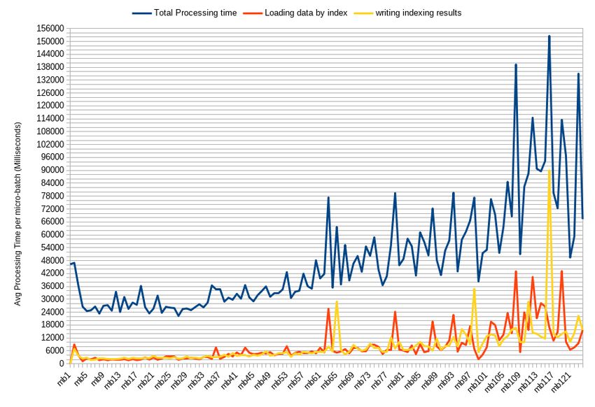
loaded data for each size of dataset shows in Figure 22 until 28.
Figure 21 illustrates the average time required for performing the saturation
given a micro-batch (blue line), and the average time required for the index
management (red line). Regarding the saturation, the figure shows that micro-
batches with different sizes require different times for processing. For example,
the time required for processing a 100M B microbatch is smaller compared to
the time required for processing microbatches with larger sizes. The increase
is not steady. In particular, we observe that micro-batches with 400M B and
500M B require the same processing time. This means the cluster could process
a bigger chunk of data within the given time-interval. We can also conclude that
the cluster was idle for some time when processing 400M B micro-batches.
Regarding the index management (red line), it shows that it is comparatively
small with respect to the saturation time, and it costs in the worse case less than
half a minute. Moreover, as with the saturation time, micro-batch size is not the
only factor. For example, the microbatch with a size of 600M B required more
time for maintaining the index because the number of inferred tuples was higher
compared with other microbatches, including the one with a size of 700M B.
Concerning global execution time (for all micro-batches), experiments showed
that when the number of micro-batches decreases, this time can decrease in
some cases (this happens in particular for i ∈ {1, 2, 3}, Table 5).
To summarize, the results we presented here show that it is possible to satu-
rate streams of RDF data in an incremental manner by using big data platforms,
and that our approach outperforms the state of the art.
Fig. 21: Average processing time and indexing management / micro-batchFig. 22: 100MB per Micro-Batch + Schema Fig. 23: 200MB per Micro-Batch + Schema
Fig. 24: 300MB per Micro-Batch + Schema

Fig. 25: 400MB per Micro-Batch + Schema
Fig. 26: 500MB per Micro-Batch + Schema

Fig. 27: 600MB per Micro-Batch + Schema
Fig. 28: 700MB per Micro-Batch + Schema

Table 5: Average time per micro-batch (mb). TE : Total Execution time of
whole process (minutes). PT : Average of Processing Time per micro-batch
(milliseconds). Indexing : Average of Indexing management to load instance
triples based on the received schema triples. LT : Number of loaded triples,
from already saturated data, by receiving new schema triples.

              Size # of mb TE (mins)   PT (ms)   Indexing     # LT
             100MB 260       105        34237      4568     1435032
             200MB 130        95        60080     15664     3097778
             300MB   86       93        73013     16129     6279178
             400MB   65       78        70707     12077     9840728
             500MB   52       59        67091     11212     11328902
             600MB   43       88       127669     33328     12717641
             700MB   37       88       102135     16152     15911994
To summarize, the results we presented here show that it is possible to reason
over streams of RDF data in an incremental manner by using big data platforms,
and that our approach outperforms the state of the art.
7 Related Work
RDF Saturation Using Big data Platforms To the best of our knowledge,
the first proposal to use big data platforms, and MapReduce in particular, to
scale the saturation operation is [12], but the authors did not present any ex-
perimental result. Other works then addressed the problem of large-scale RDF
saturation by exploiting big data systems such as Hadoop and Spark, (see e.g.,
[20, 19, 7]). For example, Urbani et al. [20, 19] proposed a MapReduce-based dis-
tributed reasoning system called WebPIE. In doing so, they identified the order
in which RDFS rules can be applied to efficiently saturate RDF data. Moreover,
they specified for each of the RDFS rule how it can be implemented using map
and/or reduce functions, and executed over the Hadoop system. Building on the
work by Urbani et al., the authors of Cichlid [7] implemented RDF saturation
over Spark using, in addition to map and reduce, other transformations that are
provided by Spark, such as filter, union, etc. Cichlid has shown that the use of
Spark can speed up saturation wrt the case when Hadoop is used. Our solution
builds and adapts the solutions proposed by WebPie and Cichlid to cater for the
saturation of streams of massive RDF data.
Incremental Saturation The problem of incremental saturation of RDF data
has been investigated by a number of proposals (see e.g., [21, 3, 5, 6, 19]). For ex-
ample, Volz et al. investigated the problem of maintenance of entailments given
changes at the level of the RDF instances as well as at the level of the RDF
schema [21]. In doing so, they adapted a previous state of the art algorithm for
incremental view maintenance proposed in the context of deductive database
[17]. Barbieri et al. [3] builds on the solution proposed by Volz et al. by consid-
ering the case where the triples are associated with an expiration date in the
context of streams (e.g., for data that is location-based). They showed that the
deletion, in this case, can be done more efficiently by tagging the inferred RDF
triples with an expiration date that is derived based on the expiration dates of
the triples used in the derivation. While Volz et al. and Barbieri et al. [3] seek to
reduce the effort required for RDF saturation, they do not leverage any indexing
structure to efficiently perform the incremental saturation. As reported by the
Volz et al. in the results of their evaluation study, even if the maintenance was
incremental, the inference engine ran out in certain cases of memory. Regarding,
Barbieri et al. [3], they considered in their evaluation a single transitive rule
(Section 5 in [3]), and did not report on the size of the dataset used, nor the
micro-batch size.
Chevalier et al. proposed Slider, a system for RDF saturation using a dis-
tributed architecture [5]. Although the objective of Slider is similar to our work,
it differs in the following aspects. First, in Slider, each rule is implemented inYou can also read