Response of middle atmospheric temperature to the 27 d solar cycle: an analysis of 13 years of microwave limb sounder data
←
→
Page content transcription
If your browser does not render page correctly, please read the page content below
Atmos. Chem. Phys., 20, 1737–1755, 2020
https://doi.org/10.5194/acp-20-1737-2020
© Author(s) 2020. This work is distributed under
the Creative Commons Attribution 4.0 License.

Response of middle atmospheric temperature to the 27 d solar cycle:
an analysis of 13 years of microwave limb sounder data
Piao Rong1,2,3,4 , Christian von Savigny4 , Chunmin Zhang1,2,3 , Christoph G. Hoffmann4 , and Michael J. Schwartz5
1 School  of Science, Xi’an Jiaotong University, 28 Xianning West Road, 710049 Xi’an, China
2 Institute of Space Optics, Xi’an Jiaotong University, 28 Xianning West Road, 710049 Xi’an, China
3 Key Laboratory for Nonequilibrium Synthesis and Modulation of Condensed Matter, Xi’an Jiaotong University,

Ministry of Education, 28 Xianning West Road, 710049 Xi’an, China
4 Institute of Physics, University of Greifswald, Felix-Hausdorff-Str. 6, 17489 Greifswald, Germany
5 Jet Propulsion Laboratory, California Institute of Technology, Pasadena, 91109 CA, USA

Correspondence: Chunmin Zhang (zcm@xjtu.edu.cn)

Received: 27 August 2019 – Discussion started: 9 September 2019
Revised: 10 December 2019 – Accepted: 6 January 2020 – Published: 13 February 2020

Abstract. This work focuses on studying the presence and          1   Introduction
characteristics of 27 d solar signatures in middle atmospheric
temperature observed by the microwave limb sounder (MLS)          The 27 d solar cycle is caused by the differential rotation of
on NASA’s Aura spacecraft. The 27 d signatures in tempera-        the sun, which leads to apparent variations in solar flux with
ture are extracted using the superposed epoch analysis (SEA)      a period of about 27 d (e.g., Sakurai, 1980, and references
technique. We use time-lagged linear regression (sensitivity      therein). Previous studies have identified 27 d solar signa-
analysis) and a Monte Carlo test method (significance test) to    tures in many different atmospheric parameters, e.g., noctilu-
explore the dependence of the results on latitude and altitude,   cent clouds (e.g., Robert et al., 2010), mesospheric water va-
solar activity, and season, as well as on different parameters    por (e.g., Thomas et al., 2015), tropical upper stratospheric
(e.g., smoothing filter, window width and epoch centers). Us-     ozone (e.g., Hood, 1986; Fioletov, 2009), the middle atmo-
ing different parameters does impact the results to a certain     spheric odd hydrogen species (e.g., Wang et al., 2015), upper
degree, but it does not affect the overall results. Analyzing     mesospheric atomic oxygen (Lednyts’kyy et al., 2017) and
the 13-year data set shows that highly significant 27 d so-       especially in temperature (e.g., Ebel et al., 1986; Hood, 1986;
lar signatures in middle atmospheric temperature are present      Keating et al., 1987; Hood et al., 1991; Hall et al., 2006; Dyr-
at many altitudes and latitudes. A tendency to higher tem-        land and Sigernes, 2007; Robert et al., 2010; von Savigny
perature sensitivity to solar forcing in the winter hemisphere    et al., 2012; Thomas et al., 2015; Hood, 2016; Beig, 2002;
compared to the summer hemisphere is found. In addition,          Beig et al., 2008) in the middle atmosphere. The term “mid-
the sensitivity of temperature to 27 d solar forcing tends to     dle atmosphere” refers to the height region of approximately
be larger at high latitudes than at low latitudes. For 11-year    15–90 km and comprises the stratosphere and mesosphere.
solar minimum conditions no statistically significant iden-       While a significant number of experimental studies investi-
tification of a 27 d solar signature is possible at most alti-    gated 27 d solar-driven variations in stratospheric and meso-
tudes and latitudes. Several results we obtained suggest that     spheric parameters, further characteristics of these signatures
processes other than solar variability drive atmospheric tem-     are yet to be discovered. Therefore, it has become a highly
perature variability at periods around 27 d. Comparisons of       interesting subject to study atmospheric variations due to the
the obtained sensitivity values with earlier experimental and     27 d solar activity cycle in middle atmospheric parameters.
model studies show good overall agreement.                           First, we briefly outline the existing experimental and
                                                                  modeling studies on 27 d solar periodicities in temperature
                                                                  of the middle atmospheric region.

Published by Copernicus Publications on behalf of the European Geosciences Union.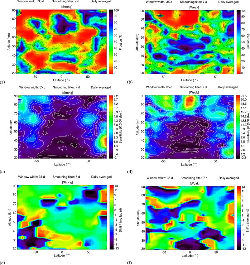
1738                                    P. Rong et al.: Response of middle atmospheric temperature to the 27 d solar cycle

    Ebel et al. (1986) reported observations of solar-driven      tions on the chemical composition and temperature of the
temperature deviations of about 1.5 K at 80 km in the trop-       middle atmosphere as simulated by the three-dimensional
ics and argue that since the response to solar activity (27       chemistry–climate model HAMMONIA. They found that the
and 13 d) is mainly determined by the dynamical proper-           response sensitivities of temperature to solar activity gener-
ties of the middle atmosphere, the strongest perturbations        ally decrease when the forcing increases, and in the extra-
should occur at middle and higher latitudes. The analysis         tropics the response was found to be seasonally dependent,
covers the years from 1975 to 1978 and is based on temper-        with typically higher sensitivities in winter than in summer.
ature measurements with the Nimbus 6 Pressure Modulator           Robert et al. (2010) identified a 27 d solar-driven signature in
Radiometer (PMR). Keating et al. (1987) also identified a         mesospheric temperatures at middle and high latitudes dur-
27 d signal in tropical mesospheric temperature (50–70 km)        ing hemispheric summer applying a cross-correlation analy-
in the 1980s using Nimbus 7 Stratosphere And Mesosphere           sis on the Microwave Limb Sounder (MLS)/Aura measure-
Sounder (SAMS) temperature data and found a maximum               ments. von Savigny et al. (2012) reported on a 27 d signa-
sensitivity at 70 km. Hood (1986) used Nimbus-7/SAMS              ture in equatorial mesopause (87 km) temperatures derived
temperature measurements (24 December 1978 to 20 May              from Envisat’s SCIAMACHY (SCanning Imaging Absorp-
1981) at low latitudes (25◦ S to 25◦ N) to determine the tem-     tion spectroMeter for Atmospheric CHartographY) observa-
perature sensitivity to solar forcing at the 27 d scale for al-   tions of the OH(3–1) Meinel band in the terrestrial nightglow.
titudes ranging from about 24 to 57 km, yielding a maxi-          Thomas et al. (2015) investigated 27 d solar-driven variations
mum temperature response amplitude of 0.36 % (∼ 1 K) near         in temperature profiles in the high-latitude summertime re-
the stratopause. The peak-to-peak variations in the 205 nm        gion for altitudes between 70 and 90 km and observed with
flux were as large as 6 % on the 27 d timescale during their      the Solar Occultation for Ice Experiment (SOFIE) on the
study period. Later, Hood et al. (1991) presented an anal-        Aeronomy of Ice in the Mesosphere (AIM) satellite. Hood
ysis of 4.3 years (24 December 1978 to 9 June 1983) of            (2016) analyzed daily ERA-Interim reanalysis data for three
Nimbus-7/SAMS temperature data for estimating and char-           separate solar maximum periods and confirmed the existence
acterizing the response of mesospheric temperature to so-         of a temperature response to 27 d solar ultraviolet variations
lar ultraviolet variations at the 27 d scale. They found that     at tropical latitudes in the lower stratosphere (15–30 km).
the maximum low-latitude temperature response amplitudes             The influence of 27 d variability on tropospheric parame-
(approximately 1.3 K for the maximum observed Lyman-α             ters has also previously been discussed (e.g., Hoffmann and
flux change of ∼ 29 %) occur at a level of ∼ 0.06 mbar, ap-       von Savigny, 2019 and references therein), but this work fo-
proximately 68 km altitude, in agreement with Keating et al.      cuses specifically on the middle atmosphere, so the tropo-
(1987). Brasseur (1993) used a two-dimensional chemical–          sphere is not discussed here.
dynamical–radiative model of the middle atmosphere to in-            While the works cited above have found correlations be-
vestigate the potential changes in temperature in response to     tween 27 d variations of solar spectral irradiance and atmo-
the 27 d variation in the solar ultraviolet flux. They found      spheric temperature variability in numerous observational
that the largest temperature response amplitude (approxi-         and modeling data sets, there is still work to be done in char-
mately 0.37 K) is at the stratopause corresponding to a peak-     acterizing and quantifying the significance of observed 27 d
to-trough solar variation of 3.3 % at 205 nm. The temperature     signatures.
sensitivity using their model for equatorial regions is 0.01 K       This paper investigates the presence and characteristics of
per % at 30 km, 0.06 K per % at 40 km and 0.12 K per %            27 d solar signatures in middle atmosphere temperature ob-
at 60 km, and the modeled sensitivity for altitudes ranging       served by the Microwave Limb Sounder (MLS). The MLS
from 40 to 60 km is in agreement with Keating et al. (1987).      data set is uniquely suited for this purpose, because it pro-
The temperature response to solar variability has not been        vides global daily coverage and covers more than an 11-
considered at altitudes above 60 km in Brasseur (1993), be-       year solar cycle. We employ the solar Mg II index as the
cause several radiative processes specific to the mesosphere      solar proxy. In this study, the superposed epoch analysis
had not been treated in detail. Zhu et al. (2003) investigated    (SEA), time-lagged linear regression (sensitivity analysis)
the ozone and temperature responses in the upper strato-          and a Monte Carlo test method (significance test) are used.
sphere and mesosphere through analytic formulations and           To investigate the robustness of the results, their dependence
the Johns Hopkins University Applied Physics Laboratory           on parameters of the analysis methods (e.g., smoothing filter,
(JHU/APL) two-dimensional chemical–dynamical coupled              window width and epoch centers), on the time of measure-
model, showing an increasing sensitivity of temperature to        ment (e.g., temperature observation time, solar activity and
the solar UV forcing with increasing latitude and altitude.       season) and on latitude and altitude are investigated.
Hall et al. (2006) and Dyrland and Sigernes (2007) iden-             The remainder of the paper is organized as follows: Sect. 2
tified signatures with periods of near 27 d in winter time        describes the MLS temperature data set and the Mg II index
meteor radar temperature time series at 90 km and for lat-        data used in this study; Sect. 3 describes the analysis pro-
itudes of 70 and 78◦ N. Gruzdev et al. (2009) analyzed            cess and the main features of the SEA, the sensitivity analy-
the effects of the solar rotational (27 d) irradiance varia-      sis and the significance test; in Sect. 4 the analysis results are

Atmos. Chem. Phys., 20, 1737–1755, 2020                                             www.atmos-chem-phys.net/20/1737/2020/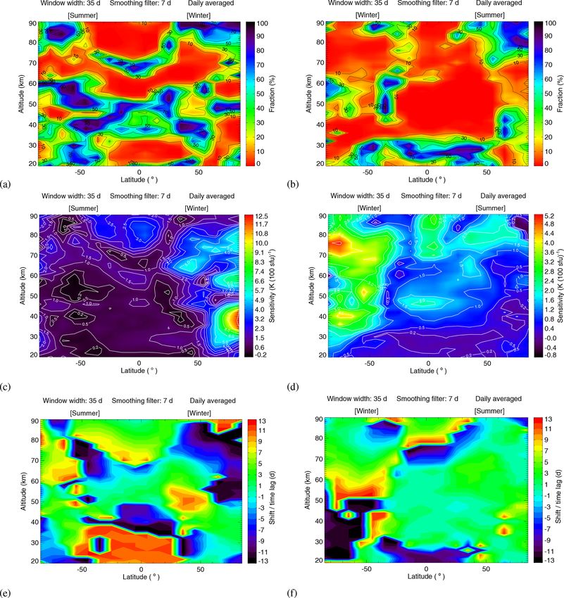
P. Rong et al.: Response of middle atmospheric temperature to the 27 d solar cycle 1739
presented, discussed and compared to earlier studies; Con-
clusions are provided at the end.
2 Data sets
2.1 Mg II Index
The core-to-wing ratio of the Mg II doublet (280 nm) in the
solar irradiance spectrum, i.e., Mg II index, is frequently
used as a proxy for tracking solar activity from the ultravi-
olet (UV) to the extreme ultraviolet (EUV) associated with
the 11-year solar cycle (22-year magnetic cycle) and solar
rotation 27 d cycle (Cebula and Deland, 1998; Dudok de Wit
et al., 2009). In contrast to other solar proxies (such as the
Lyman-α and the F10.7 cm radio flux), the Mg II index is
used here because the Mg II best correlates with solar UV
radiation variation, particularly during solar minimum con-
ditions (Dudok de Wit et al., 2009; Snow et al., 2014).
The Mg II index is a dimensionless proxy. The relationship
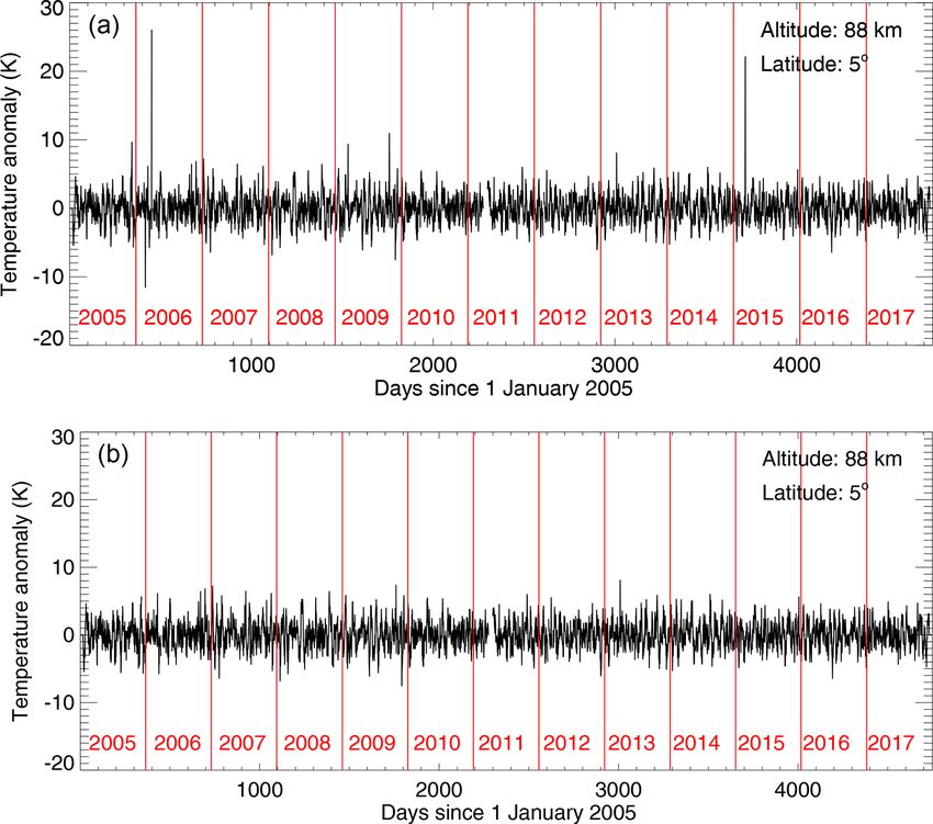
Figure 1. (a) Mg II index data from 2005 to 2017. (b) Time series of
between the Mg II index and other solar proxies, e.g., the zonally and daily averaged temperature for the 5◦ N (i.e., 0–10◦ N)
Lyman-α or the F10.7 cm radio flux, can be easily established latitude bin at 88 km derived from MLS on Aura. Data gaps occur
by a linear regression (e.g., von Savigny et al., 2012, 2019). on the days 453–458, 555, 2276–2298, 2605–2609 and 2630–2635.
The F10.7 cm radio flux is usually given in solar flux units
(sfu), which are equal to 10−22 W m−2 Hz−1 . This allows the
results to be compared with other research results. mation in the stratosphere and above (from 90 km down to
For this study we employ the Bremen daily Mg II about 16 km) (Livesey et al., 2018).
index composite data set as the solar proxy, which is In this work, we use the MLS Level 2 temperature prod-
available from 1978 to present and derived from six uct version 4.2. MLS temperature is available from 2 August
data sets, i.e., the Solar Backscatter UltraViolet Radiome- 2004 to present. The precision and accuracy of the MLS tem-
ter (SBUV) (before 1995), the Global Ozone Monitoring perature data product are shown in Table 3.22.1 of Livesey
Experiment (GOME) (1995–2011), SCIAMACHY (2002– et al. (2018). The precision is 1 K or better in the tropo-
2012), GOME-2A (since 2007), GOME-2B (since 2012) and sphere and lower stratosphere (from 261 to 3.16 hPa), de-
GOME-2C (since 2019). The most recent information on the grading to 3.6 K in the upper mesosphere (at 0.001 hPa).
Mg II data can be found in Snow et al. (2014). Figure 1a The observed biases based upon comparisons with analyses
shows the Mg II index data from 2005 to 2017 that are used and other previously validated satellite-based measurements
in this analysis. range from −2.5 to +1 K in the troposphere and lower strato-
sphere, increasing to −9 K at the highest altitude. The recom-
2.2 MLS on Aura mended useful vertical range for scientific studies is between
261 hPa (10 km) and 0.001 hPa (96 km), and the vertical reso-
The National Aeronautics and Space Administration lution varies between 3.6 km (at 31.6 hPa) and 13–14 km (at
(NASA) Earth observation satellite Aura has been in a 0.001 hPa). The horizontal resolution is ∼ 165 km between
near-polar 705 km altitude orbit since 2004. The Microwave 261 hPa and 0.1 hPa and degrades to 280 km at 0.001 hPa.
Limb Sounder (MLS) on Aura consists of seven radiome- To investigate the presence of a 27 d solar cycle signature in
ters observing emission in the 118 GHz, 190 GHz, 240 GHz, the temperature data set and to keep the annual data com-
640 GHz and 2.5 THz regions. The MLS measurements pro- plete, the period from 1 January 2005 to 31 December 2017
vide vertical profiles of temperature, geopotential height, was selected as shown in Fig. 1b. In the following analysis,
several atmospheric trace species and ice water content of we first employ the daily and nightly averaged MLS temper-
clouds with near-global coverage on a daily basis (Waters et ature data. In Sect. 4.1.1 and 4.2.1 we investigate how the
al., 2006; Livesey et al., 2018). results change if daytime (or nighttime) measurements only
MLS temperature is retrieved primarily from MLS mea- are employed for the analysis.
surements of the thermal emission of O2 near 118 and
240 GHz (Schwartz et al., 2008). The isotopic 240 GHz line
is the primary source of temperature information in the tro-
posphere (extending the profile down to about 9 km), while
the 118 GHz line is the primary source of temperature infor-
www.atmos-chem-phys.net/20/1737/2020/ Atmos. Chem. Phys., 20, 1737–1755, 2020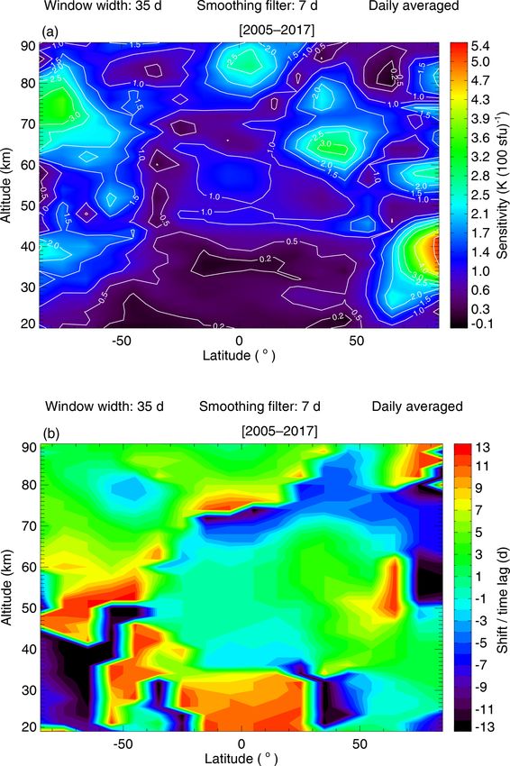
1740 P. Rong et al.: Response of middle atmospheric temperature to the 27 d solar cycle
Figure 2. Flow chart of the analysis procedure and the input and
output parameters.
3 Methodology
The approach employed to analyze the 27 d solar cycle signal
in temperature is illustrated in Fig. 2. First, temperature and
Mg II index anomalies are calculated (see Sect. 3.1). Next,
the SEA method is applied to the temperature and Mg II in-
dex anomalies to obtain the epoch-averaged temperature and
Mg II index anomalies (Sect. 3.2). Then, the epoch-averaged
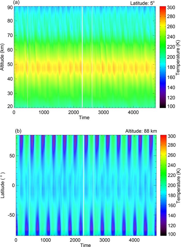
Figure 3. (a) The MLS temperature as a function of altitude and
temperature and Mg II index anomalies are used to perform
time day at 5◦ N. (b) The MLS temperature as a function of latitude
the sensitivity analysis (Sect. 3.3) and the significance test and time at 88 km altitude. The white lines indicate data gaps.
(Sect. 3.4). The individual steps are described in detail in the
corresponding subsections.
In the process, different input observational and statistical averaged daily and zonally for each altitude and latitude bin
parameters may affect the results. For example, the results between 1 January 2005 and 31 December 2017.
may depend on whether daytime, nighttime or daily averaged Figure 1b shows the daily averaged temperature data for
MLS temperature data are used for the analysis. Other pa- an altitude of 88 km and a latitude of 5◦ N (averaged zon-
rameters that may affect the results are latitude and altitude, ally and over the 0–10◦ N latitude range). There are five data
the width of the window used in the data preprocessing, the gaps and six abnormal peaks. The data gaps occur in the fol-
choice of the epoch centers (maxima or minima of Mg II in- lowing periods: days 453–458 (6 d gap in 2006), day 555
dex anomalies) applied for the SEA, and the smoothing filter (1 d gap in 2006), days 2276–2298 (23 d gap in 2011), days
used to choose the maxima or minima as epoch centers. In 2605–2609 (5 d gap in 2012) and days 2630–2635 (6 d gap in
addition, the dependence of the results on solar activity and 2012). Days are counted starting with 1 January 2005. These
season also needs to be discussed. To check how these pa- gaps exist in the observations at all latitudes and altitudes
rameters affect the results, different tests are performed and (see Fig. 3). The white lines in Fig. 3 indicate that tempera-
described in Sect. 4. ture data are missing. The outliers/abnormal peaks visible in
Fig. 1b occur on days 341, 417, 452, 1532, 1759 and 3717.
3.1 Data preprocessing Note that the outliers appear on different days for different
altitudes and latitudes. In order to investigate the presence of
We defined a standard altitude grid with 36 levels from 20 to a 27 d solar cycle signature in the temperature data set, it is
90 km with a step size of 2 km and a standard latitude grid necessary to avoid the invalid points (temperature gaps and
with 18 bins from 90◦ S to 90◦ N with a step size of 10◦ . outliers) in the SEA. This can be easily implemented in the
MLS geopotential height was converted to geometric height SEA by ignoring the data gaps and outliers in the averaging
using the height- and latitude-dependent formula provided procedure (see below).
by Roedel and Wagner (2011). The temperature data were
Atmos. Chem. Phys., 20, 1737–1755, 2020 www.atmos-chem-phys.net/20/1737/2020/
P. Rong et al.: Response of middle atmospheric temperature to the 27 d solar cycle                                                1741

                                                                       anomalies as shown in Fig. 6. The red, blue and green points
                                                                       represent the local maxima identified for the 0, 7 and 13 d
                                                                       smoothed Mg II index anomalies, respectively. We discuss
                                                                       the impact of the smoothing filter on the results in Sect. 4.1.1
                                                                       and 4.2.1. A similar method can be applied to choose the
                                                                       minima in the Mg II index times series, and we compare the
                                                                       variation in the results by utilizing the maxima or minima of
                                                                       Mg II index anomalies for the SEA in Sect. 4.1.1 and 4.2.1.
                                                                          Second, we choose 61 d centered at these solar maxima
                                                                       dates as an analysis epoch (i.e., 30 d before and after these
                                                                       maxima). The whole time series from 1 January 2015 to
                                                                       31 December 2017 will be divided into N epochs, and each
                                                                       epoch covers 61 d. Finally, the epoch-averaged temperature
                                                                       anomaly (Tanomaly [x]) is obtained by averaging N temper-
                                                                                 x
                                                                       atures (Tepoch ) of the corresponding day (x) in each 61 d
                                                                       epoch, see Eq. (1).
                                                                                              N
                                                                                        1     X
                                                                                                        x
                                                                       Tanomaly [x] =                 Tepoch                        (1)
                                                                                        N   epoch=1
Figure 4. (a) The MLS temperature anomalies generated by sub-
tracting a 35 d running mean from the time series for an altitude of   Here, x represents an integer between −30 and 30. Simi-
88 km and a latitude of 5◦ N. (b) Similar to (a) except for avoid-     larly, the epoch-averaged Mg II anomaly is determined this
ing the abnormal peaks on the days 341, 417, 452, 1532, 1759 and
                                                                       way. Figure 7a displays an example of the resulting epoch-
3717. The plots are based on daily averaged temperature data.
                                                                       averaged temperature (at 88 km and 5◦ N) and Mg II index
                                                                       anomalies. The Mg II index anomaly exhibits very symmet-
   Next, we apply a 35 d running mean and then calculate the           ric behavior with a maximum at zero day time lag and min-
anomalies as the deviation from the running mean for MLS               ima near ±13 d, as expected. The epoch-averaged tempera-
temperature and the Mg II index time series. The resulting             ture anomaly also shows a clear maximum but with a time lag
temperature anomalies for an altitude of 88 km and a latitude          of 2 d, indicating that the response in mesospheric tempera-
of 5◦ N are shown in Fig. 4a. We define outliers as data points        ture to the solar forcing occurs with a time lag. The obtained
for which the magnitude of the temperature anomaly exceeds             epoch-averaged temperature and Mg II index anomalies (un-
4 times the standard deviation of the anomaly time series.             smoothed) are used in the sensitivity analysis. A 3 d smooth-
Figure 4b shows the temperature anomaly with removed out-              ing is applied to epoch-averaged temperature and Mg II index
liers. The width of the smoothing window is chosen as 35 d             anomalies for the significance test.
to remove the seasonal modulation of the temperature signal
                                                                       3.3   Sensitivity analysis
while leaving the variation at shorter timescales unaltered. In
Sect. 4.1.1 and 4.2.1 we investigate how the results change if         The resulting epoch-averaged temperature and Mg II index
different window widths (e.g., 27 and 50 d) are employed for           anomalies are used to determine the sensitivity of middle at-
the analysis. Those steps above are a preparation for the sub-         mospheric temperature to changes in the solar activity rep-
sequent SEA, significance testing and sensitivity analysis.            resented here by the Mg II index. The relationship between
                                                                       temperature anomaly (Tanomaly [x]) and Mg II index anomaly
3.2   Superposed epoch analysis (SEA)
                                                                       (Mg IIanomaly [x]) can be represented by a linear regression
To identify weak 27 d solar signatures in temperature time             line (see Eq. 2) if the maxima in the epoch-averaged anoma-
series affected by variability from various sources, the su-           lies occur at the same time lag. The sensitivity is directly de-
perposed epoch analysis method (SEA) (e.g., Howard, 1833;              termined by the slope (k) of a linear regression line to the
Chree, 1912) is an effective choice. The SEA is applied to             data points, i.e., un-smoothed epoch-averaged temperature
the time series covering the period from January 2005 to De-           and Mg II index anomalies.
cember 2017.                                                           Tanomaly [x] = b + k × Mg IIanomaly [x]                      (2)
   An overview of the SEA is shown in Fig. 5. First, the epoch
centers need to be chosen. The local maxima in the Mg II                  However, as shown in Fig. 7a, there is a time lag or shift (l)
index time series – reflecting maxima in solar spectral irradi-        between solar maximum and temperature maximum. If the
ance – can be used as the epoch centers (represented as Max 1          times of the maxima do not coincide, then an ellipse is fitted
to Max N in Fig. 5). The Mg II index maxima are identified             instead of a straight line. To remove the phase shift between
in the un-smoothed (0 d) or 7 or 13 d smoothed Mg II index             the two anomalies, we need to shift the temperature curve

www.atmos-chem-phys.net/20/1737/2020/                                                       Atmos. Chem. Phys., 20, 1737–1755, 2020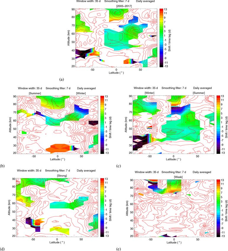
1742                                      P. Rong et al.: Response of middle atmospheric temperature to the 27 d solar cycle

Figure 5. Overview of the superposed epoch analysis (SEA). It should be noted that the epochs are allowed to overlap even though we do
not show it in the figure.

                                                                      Tanomaly [x + l] = b + k × Mg IIanomaly [x]                 (3)

                                                                         The phase lag (l) can be determined by time-lagged cross-
                                                                      correlation as shown in Fig. 7b. The sensitivity for this par-
                                                                      ticular combination of altitude and latitude is obtained by
                                                                      shifting the epoch-averaged temperature anomaly backwards
                                                                      by 2 d, i.e., l = −2, see Fig. 7c. The sensitivity obtained
                                                                      for a 35 d window width, a 7 d smoothing filter and using
                                                                      maxima of the Mg II index anomaly as the epoch centers
                                                                      is 190 (±15) K per (Mg II index unit). The relationship be-
                                                                      tween the Mg II index and the F10.7 cm radio flux was estab-
                                                                      lished by a linear regression to annually averaged values for
                                                                      the years 2003 to 2010 – 1MgII / 1F10.7 = 0.0135 Mg II
                                                                      index unit (100 sfu)−1 – and the sensitivity value translates
                                                                      to 2.57 (±0.20) K (100 sfu)−1 . The result is in very good
                                                                      agreement with the conclusion of von Savigny et al. (2012).
                                                                      They analyzed zonally averaged OH(3–1) rotational tem-
Figure 6. (a) Mg II index anomalies generated by subtracting a 35 d
                                                                      peratures at 87 km for the [0, 20◦ N] latitude range using
running mean from the time series. The black line presents the un-
smoothed or 0 d smoothed Mg II index anomaly. The red, blue and
                                                                      the Mg II index derived from SCIAMACHY and found
green points are the local maxima chosen from the 0, 7 and 13 d       a temperature sensitivity to solar forcing in terms of the
smoothed Mg II index anomalies, respectively. (b) Similar to (a)      27 d solar cycle of 182 (±69) K per (Mg II index unit) or
except for the year 2005 only. In addition, the red, blue and green   2.46 (±0.93) K (100 sfu)−1 . We need to point out, however,
lines present the Mg II index anomalies smoothed by a 0, 7 and 13 d   that von Savigny et al. (2012) analyzed a much more limited
running mean, respectively.                                           time period – i.e., from April 2005 to October 2006 – com-
                                                                      pared to the results presented here. More comparisons of our
                                                                      sensitivity results to previously published ones are presented
by l d to obtain the time-lagged epoch-averaged temperature           in Sect. 4.2.2 and 4.2.3.
anomalies Tanomaly [x + l]. Then the sensitivity parameter (k)
is derived from Eq. (3).

Atmos. Chem. Phys., 20, 1737–1755, 2020                                                www.atmos-chem-phys.net/20/1737/2020/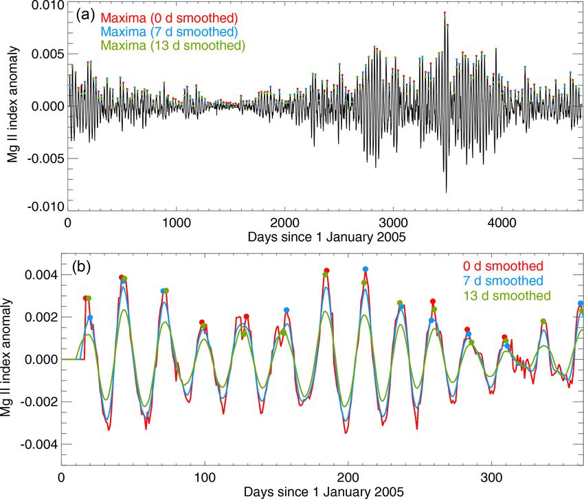
P. Rong et al.: Response of middle atmospheric temperature to the 27 d solar cycle                                                    1743

Figure 7. (a) Epoch-averaged Mg II index and temperature anomalies for a total of 173 epochs. The dashed red line is the epoch-averaged
Mg II index anomaly multiplied by a factor of 220. The solid thin blue line corresponds to the epoch-averaged temperature anomaly. The solid
bold blue line represents the temperature anomaly smoothed with a 3 d running mean. The black line is a sinusoidal fit to the 3 d smoothed
epoch-averaged temperature anomaly, with an amplitude of 0.28 K. (b) Cross correlation between the 61 d epoch-averaged temperature and
Mg II index anomaly time series (the results correspond to the 35 d running mean) for the time lag between −30 and +30 d. (c) Scatter plot
of the 2 d lagged temperature and Mg II index anomalies based on the epoch averages displayed in (a). The black line represents the fitted
linear regression line.

3.4   Significance testing

We use a similar Monte Carlo test method as is used in von
Savigny et al. (2019) to examine the significance of the ob-
tained results. Instead of using local solar maxima as the
epoch centers in the SEA, the epoch centers are chosen ran-
domly, and the SEA is repeated. The number of random
epochs is the same as in the actual SEA. This procedure is
carried out 1000 times. Then a sinusoidal function is used
to fit every single random realization of the 3 d smoothed
epoch-averaged temperature anomaly. Comparing the am-
plitude of the fitted sinusoidal function of the 1000 random            Figure 8. Illustration of the Monte Carlo significance test for an
                                                                        altitude of 88 km and a latitude of 5◦ N. The red line shows the am-
cases to the amplitude of the actual case, the statistical sig-
                                                                        plitude of a sinusoidal fit to the extracted 27 d signatures in MLS
nificance of the SEA results can be evaluated. The amplitude            daily averaged temperature. The black line shows the fitted ampli-
and phase of fitted sinusoidal functions, as well as the frac-          tudes to epoch-averaged temperature anomalies for 1000 randomly
tion of random realizations with amplitudes larger than ac-             chosen epoch ensembles.
tual data are the results of the significance test. If the fraction
of random realizations with amplitudes larger than the ampli-
tude of the actual SEA is close to zero, then the 27 d signature        lies, which were obtained by subtracting a 35 d running mean
in MLS temperature data is likely not a spurious signature.             from the daily Mg II index data.
Figure 8 shows the results of the Monte Carlo significance
test at 88 km and 5◦ N. The local solar maxima used here are
determined based on the 7 d smoothed Mg II index anoma-

www.atmos-chem-phys.net/20/1737/2020/                                                      Atmos. Chem. Phys., 20, 1737–1755, 2020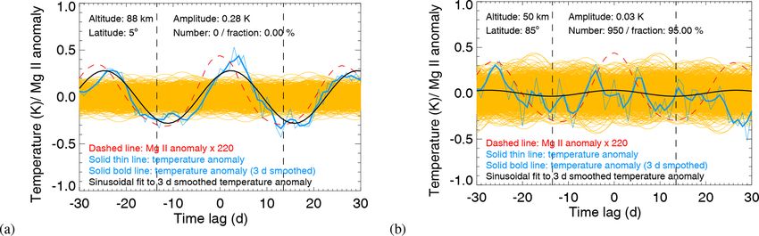
1744                                    P. Rong et al.: Response of middle atmospheric temperature to the 27 d solar cycle

4     Results and discussion                                       The resulting fraction of random realizations with amplitudes
                                                                   larger than the actual SEA is displayed in Fig. 9 as a function
The main purpose of the present work is to investigate the         of latitude and altitude. For the results shown in Fig. 9a, the
presence and characteristics of 27 d solar signatures in the       local solar maxima used in the SEA are chosen from the 7 d
middle atmosphere temperature observed by MLS. In order            smoothed Mg II index anomalies obtained by subtracting a
to investigate how robust the results are, different tests were    35 d running mean from the Mg II index data. The tempera-
performed, i.e., a significance test, a sensitivity test, and an   ture anomalies used in the SEA are obtained by subtracting a
investigation of the dependence of the results on real geo-        35 d running mean from the daily averaged temperature time
physical parameters (i.e., solar activity, season, latitude and    series. As shown in the figure, there exists a complex pattern
altitude) and on statistical/numerical parameters (i.e., win-      of latitude/altitude regions with low fractions indicating that
dow width, epoch centers and smoothing filter).                    the identified 27 d signatures are most likely not caused spu-
                                                                   riously – making a solar origin likely. As shown in the figure,
4.1     Significance test results                                  fractions of less than 10 % (high significance) appear in the
                                                                   tropics for the altitude range of 40–60 and 80–90 km, as well
The significance testing method was described in Sect. 3.4.
                                                                   as at 40◦ N for the altitude of about 65 km. The high signifi-
To investigate the dependence of the significance results on
                                                                   cance also appears at the high latitudes, e.g., at 70–85◦ S for
altitude and latitude, the width of the window, epoch centers
                                                                   the altitude ranges of 30–40 and 60–80 km and at 80–85◦ N
and the temperature observations, these tests were performed
                                                                   for altitudes of around 40 km.
at each altitude and latitude, for different window widths of
                                                                       In addition, Fig. 10 provides two examples of high- and
27, 35 and 50 d, as well as different local maxima chosen by
                                                                   low-significance cases. Figure 10a shows the epoch-averaged
0 or 7 or 13 d smoothed Mg II index anomalies, for daytime,
                                                                   Mg II index and temperature anomalies and the sinusoidal fit
nighttime and daily averaged temperature observations.
                                                                   to the 3 d smoothed epoch-averaged temperature anomalies
                                                                   for the actual SEA and for 1000 randomly chosen epoch en-
4.1.1    Dependence of the results on statistical
                                                                   sembles at 88 km for a latitude of 5◦ N. There is no random
         parameters
                                                                   sinusoidal fit amplitude larger than the actual one, that is, the
The dependence of the results on the different parameters is       fraction of the significance test is 0.0 %. Figure 10b is a sig-
carried out based upon temperature data in the tropical (5◦ N)     nificance test result for an altitude of 50 km and a latitude of
mesopause region (88 km). Table 1 lists the results for the        85◦ N. In this case 95.0 % of the random sinusoidal fit ampli-
different statistical parameters considered and for the differ-    tudes are larger than the amplitude of the actual analysis.
ent observational temperature (daytime, nighttime and daily            In order to check the influence of the input parameters on
averaged temperature) data sets. The maximum and mini-             the results at different latitudes, we show in Fig. 9 the signif-
mum of the fraction of random realizations with amplitudes         icance results for some of the combinations of input parame-
larger than actual data are underlined. The max-to-min varia-      ters yielding the largest fractions of random realizations with
tion in the fraction for the daytime temperature case is larger    amplitudes larger than the actual SEA (see Table 1). The re-
than the one for the nighttime and daily averaged temperature      sults obtained using a 27 d window width and 0 d smoothing
cases. In terms of daily averaged temperature, the maximum         filter are shown in Fig. 9b. The results obtained using a 27 d
and minimum fractions are about 1.0 % and 0.0 %, respec-           window width, a 0 d smoothing filter and daytime tempera-
tively. That is, the variation in the fraction is about 1.0 %      ture data are shown in Fig. 9c. The results obtained using a
for different input parameters. For nighttime temperature,         50 d window width, a 0 d smoothing filter, nighttime temper-
the maximum and minimum fractions are about 1.9 % and              ature data and minima of Mg II index anomaly are shown in
0.0 %, respectively. The max-to-min variation in the fraction      Fig. 9d. The regions of high significance obviously become
is about 1.9 %, but for the daytime temperature, the maxi-         smaller in Fig. 9b–d, but the locations of these regions have
mum and minimum fractions are about 28.6 % and 1.5 %, re-          not changed. That means different input parameters have an
spectively. The max-to-min variation in the fraction increases     impact on the results but will not affect the overall character-
to about 27.1 %. The exact origin of this different behavior       istics.
of the daytime temperature data is currently unknown. More
discussion on the dependence of the results on statistical pa-     4.1.3   Dependence of the results on season
rameters at different latitudes and altitudes will be given in
Sect. 4.1.2.                                                       To determine whether the 27 d solar cycle signal in middle
                                                                   atmospheric temperature depends on season, the SEA and the
4.1.2    Dependence of the results on latitude                     subsequent significance tests were performed for winter and
                                                                   summer separately. We assume that “winter” includes the 6
We performed the significance test for the daily averaged          months of October, November, December, January, February
temperature from 2005 to 2017 for the latitude range from          and March, and “summer” includes the other 6 months for
85◦ S to 85◦ N and the altitude range from 20 to 90 km.            the Northern Hemisphere. For the Southern Hemisphere, it

Atmos. Chem. Phys., 20, 1737–1755, 2020                                             www.atmos-chem-phys.net/20/1737/2020/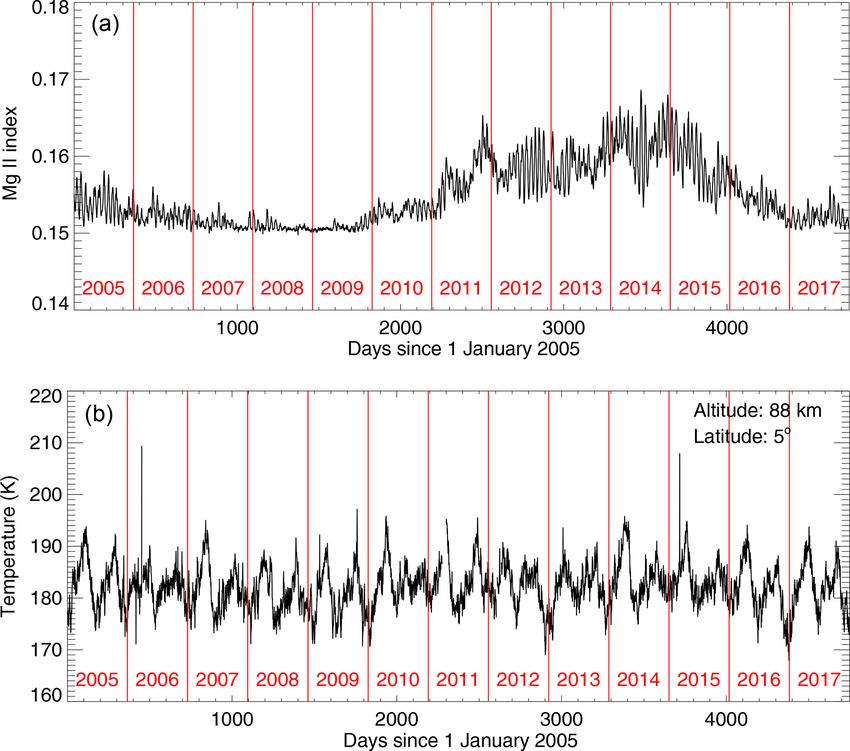
P. Rong et al.: Response of middle atmospheric temperature to the 27 d solar cycle                                                        1745

Figure 9. (a) The fraction of random realizations with amplitudes larger than the actual SEA based on the daily averaged temperature data
for latitudes ranging from 85◦ S to 85◦ N and altitudes ranging from 20 to 90 km. A 35 d window width, 7 d smoothing filter and maxima of
the Mg II index anomaly are used in this test. (b) Similar to (a) except that a 27 d window width and 0 d smoothing filter are used. (c) Similar
to (a) except that a 27 d window width, 0 d smoothing filter and daytime temperature data are used. (d) Similar to (a) except that a 50 d
window width, 0 d smoothing filter, nighttime temperature data and minima of the Mg II index anomaly are used.

Figure 10. Similar to Fig. 7a except that the orange lines are a sinusoidal fit to the 3 d smoothed epoch-averaged temperature anomalies for
1000 randomly chosen epoch ensembles. (a) For an altitude of 88 km and a latitude of 5◦ N. (b) For an altitude of 50 km and a latitude of
85◦ N.

www.atmos-chem-phys.net/20/1737/2020/                                                        Atmos. Chem. Phys., 20, 1737–1755, 2020
1746                                          P. Rong et al.: Response of middle atmospheric temperature to the 27 d solar cycle

Table 1. Significance testing results for different input parameters used in the analysis. The temperature data at a latitude of 5◦ N and altitude
of 88 km are used here. There are two parameters shown in the table. The first one is absolute amplitude in K of the fitted sinusoidal function.
The second one is the fraction (%) of random realizations with amplitudes larger than actual data. The values in bold font correspond to the
maximum and minimum of the fraction of random realizations with amplitudes larger than the actual data for the daily averaged, the daytime
and the nighttime measurements.

                Time            Temperature        Epoch      Smoothing                       Window width
                series                             centers∗   filter       27 d                35 d              50 d
                2005–2017       daily              Maxima     0d           0.18 K, 1.0 %       0.22 K, 0.6 %     0.22 K, 0.5 %
                                averaged                      7d           0.21 K, 0.2 %       0.28 K, 0.0 %     0.25 K, 0.0 %
                                                              13 d         0.20 K, 0.5 %       0.23 K, 0.4 %     0.23 K, 0.3 %
                                                   Minima     0d           0.20 K, 0.5 %       0.25 K, 0.3 %     0.22 K, 0.4 %
                                                              7d           0.20 K, 0.4 %       0.26 K, 0.2 %     0.22 K, 0.3 %
                                                              13 d         0.21 K, 0.2 %       0.26 K, 0.2 %     0.22 K, 0.3 %
                                daytime            Maxima     0d           0.14 K, 28.6 %      0.22 K, 9.8 %     0.23 K, 4.9 %
                                                              7d           0.20 K, 6.9 %       0.27 K, 2.7 %     0.26 K, 2.4 %
                                                              13 d         0.15 K, 23.4 %      0.18 K, 20.0 %    0.16 K, 24.1 %
                                                   Minima     0d           0.23 K, 3.1 %       0.30 K, 1.5 %     0.28 K, 1.7 %
                                                              7d           0.22 K, 3.6 %       0.27 K, 3.2 %     0.18 K, 17.4 %
                                                              13 d         0.18 K, 11.4 %      0.23 K, 8.8 %     0.17 K, 22.0 %
                                nighttime          Maxima     0d           0.20 K, 0.8 %       0.25 K, 0.4 %     0.23 K, 1.6 %
                                                              7d           0.24 K, 0.0 %       0.32 K, 0.0 %     0.28 K, 0.0 %
                                                              13 d         0.25 K, 0.0 %       0.31 K, 0.0 %     0.30 K, 0.0 %
                                                   Minima     0d           0.25 K, 0.1 %       0.27 K, 0.3 %     0.22 K, 1.9 %
                                                              7d           0.23 K, 0.1 %       0.28 K, 0.1 %     0.27 K, 0.1 %
                                                              13 d         0.25 K, 0.1 %       0.30 K, 0.1 %     0.28 K, 0.1 %
              ∗ Maxima/minima of Mg II index anomaly.

is the opposite. More than three months for each season are                Hemisphere winter, leading to enhanced overall atmospheric
considered here in order to increase the number of epochs                  variability and consequently making the identification of a
available for analysis.                                                    27 d solar signature in atmospheric temperature more diffi-
   The significance testing results depending on season are                cult.
shown in Fig. 11a–b. The input parameters used in this anal-
ysis are the same as in Fig. 9a. In the Southern Hemisphere,               4.1.4    Dependence of the results on solar activity
the 27 d solar cycle signal in daily averaged temperature is
more obvious in winter than in summer. In the Northern                     In addition, we investigated the dependence of the results
Hemisphere, the 27 d signature in temperature at low lati-                 on solar activity. The comparison of the strong solar activity
tudes (below 50◦ ) for the altitude of 35–60 km is more sig-               years (2011–2014) with the weak solar activity years (2007–
nificant in summer than in winter, but for the altitude of 20–             2009) is shown in Fig. 12a–b. The input parameters used here
30 km the signature is more significant in winter. At high                 are identical with the ones for Fig. 9a. The region of high
latitudes (70–85◦ N), the 27 d signature is more significant               significance is larger for strong solar activity years than for
in winter than in summer, especially for the middle strato-                weak solar activity years. For weak solar activity years, the
sphere (30–40 km). In total, the region of high significance is            region of high significance mainly concentrates in the equa-
larger for “summer” months (October–March) than “winter”                   torial mesopause region as shown in Fig. 12b. For strong
months (April–September) for the global region.                            solar activity years, the region of high significance is more
   An important finding is that large differences exist be-                distributed over high latitudes, mainly at 70–85◦ N and 40–
tween Northern Hemisphere winter and summer. For north-                    60◦ S at around 40 km and at 70–85◦ S at around 60–80 km.
ern summer (see Fig. 11b), the latitude–altitude ranges with                  The results demonstrate that the overall significance of
fractions less than 10 % – indicative of a likely solar origin             the potential 27 d solar signatures in temperature is gener-
of the identified signatures – are significantly larger than for           ally much lower for solar minimum conditions (see Fig. 12b)
northern winter (see Fig. 11a). These differences could be                 than for solar maximum conditions (see Fig. 12a). An ex-
related to enhanced planetary wave activity during Northern                ception is the tropical mesopause region, where the fraction

Atmos. Chem. Phys., 20, 1737–1755, 2020                                                        www.atmos-chem-phys.net/20/1737/2020/
P. Rong et al.: Response of middle atmospheric temperature to the 27 d solar cycle 1747 Figure 11. (a–b) Similar to Fig. 9a, except for different seasons. (c–f) Sensitivity and shift for latitudes from 85◦ S to 85◦ N and altitudes from 20 to 90 km for different seasons. Panels (a), (c) and (e) are the results for the time range from October to March (northern winter/southern summer), and panels (b), (d) and (f) are the results for the time range from April to September (northern summer/southern winter). of random realizations with amplitudes exceeding the am- pected. It is also worth pointing out that the overall signif- plitude of the actual SEA is smaller for low solar activity icance of the results (as quantified by the latitude–altitude than for enhanced solar activity. The reasons for this behav- ranges with fractions less than 10 %) is smaller for enhanced ior are currently not understood. The general decrease in the solar activity compared to analyzing the entire data set (com- significance with decreasing solar activity is, however, as ex- pare Figs. 12a and 9a). This can be explained by the reduced www.atmos-chem-phys.net/20/1737/2020/ Atmos. Chem. Phys., 20, 1737–1755, 2020
1748                                       P. Rong et al.: Response of middle atmospheric temperature to the 27 d solar cycle

Figure 12. (a–b) Similar to Fig. 9a, except for strong and weak solar activity years. (c–f) Sensitivity and shift for latitudes from 85◦ S to
85◦ N and altitudes from 20 to 90 km for different solar activity.

number of epochs available if only parts of the time series              4.2   Sensitivity analysis
are analyzed and highlights the importance of the length of
the time series for obtaining statistically significant results.
                                                                         The temperature sensitivity to solar forcing was calculated
                                                                         with the method described in Sect. 3.3. Similar to the sig-
                                                                         nificance testing, we also investigated the dependence of the

Atmos. Chem. Phys., 20, 1737–1755, 2020                                                    www.atmos-chem-phys.net/20/1737/2020/
P. Rong et al.: Response of middle atmospheric temperature to the 27 d solar cycle 1749
sensitivity results on different input and observational param-
eters.
4.2.1 Dependence of the results on statistical
parameters
The sensitivity analysis was performed first with the temper-
ature data at the mesopause (88 km) and in the tropics (5◦ N).
Table 2 lists the sensitivity values (i.e., the slope of fitted lin-
ear regression line) and the uncertainties depending on the
different settings. The underlined values in the table repre-
sent the maximum and minimum sensitivity values for differ-
ent cases. The uncertainties are below 0.6 K (100 sfu)−1 . The
maximum of the sensitivity is 2.74 (±0.28) K (100 sfu)−1
for daily averaged temperature, 3.18 (±0.40) K (100 sfu)−1
for daytime temperature and 2.95 (±0.45) K (100 sfu)−1 for
nighttime temperature. The minimum of the sensitivity
is 1.82 (±0.27) K (100 sfu)−1 for daily averaged tempera-
ture, 1.33 (±0.34) K (100 sfu)−1 for daytime temperature and
1.81 (±0.38) K (100 sfu)−1 for nighttime temperature. The
max-to-min variation in the sensitivity value due to differ-
ent input parameters is 0.92 K (100 sfu)−1 for daily averaged
temperature, 1.85 K (100 sfu)−1 for daytime temperature and
1.14 K (100 sfu)−1 for nighttime temperature. Thus, the in-
fluence of the input parameters on the sensitivity result is rel-
atively smaller in daily averaged temperature. This feature
is in line with the results derived from the significance test
which was discussed in Sect. 4.1.1.
Overall, there is a tendency toward larger sensitivities if a
wider window is used for determining the anomalies. The ef-
fect is particularly pronounced for the cases with a 0 and 7 d
smoothing of the anomalies. This dependence of the sensi- Figure 13. The (a) sensitivity and (b) shift for all latitudes from
tivities on window width may be expected, because, for nar- 85◦ S to 85◦ N and the altitudes from 20 to 90 km, and the analysis
rower window widths, parts of the 27 d signatures present year is from 2005 to 2017.
may be removed. The same window width is, however, also
used for determining the Mg II index anomalies so that part
of this effect is compensated, reducing the effect of window sitivity generally increases with increasing altitude at low
width on the sensitivity value. It is also worth pointing out latitudes. Second, the higher sensitivity values appear near
that, for most cases, the sensitivity values for the different the poles. Near the Equator the sensitivity ranges from ∼ 0
window widths agree within combined uncertainties. to 2.80 K (100 sfu)−1 , but the maximum sensitivity occurs at
85◦ N for an altitude of about 40 km. In addition, two dis-
4.2.2 Dependence of the results on latitude tinct features are present in the 70–80 km altitude range for
southern high latitudes and around 65 km at 40◦ N.
Next, we performed the sensitivity analysis for the daily aver- When comparing the graph with the significance test re-
aged temperature from 2005 to 2017 for latitudes from 85◦ S sults shown in Fig. 9a, it can be seen that the larger sensitiv-
to 85◦ N and altitudes from 20 to 90 km. For this analysis the ity values appear in regions with lower fraction, i.e., higher
local solar maxima used in the SEA were determined based significance, as expected. Figure 13b shows the time lag be-
on the 7 d smoothed Mg II index anomalies obtained by sub- tween local solar maximum (at the 27 d scale) and the tem-
tracting a 35 d running mean from the Mg II index data. perature maximum. Comparing Fig. 13a with Fig. 13b shows
The temperature anomalies used in the SEA are obtained that small time lags tend to occur in latitude–altitude regions
by subtracting a 35 d running mean from the daily aver- with large sensitivity.
aged temperature time series. The resulting sensitivity values In Fig. 14a we show the MLS temperature sensitivity to
and shifts (time lag) are displayed in Fig. 13. The obtained 27 d solar forcing as a function of altitude for a latitude
sensitivity values range from −0.02 to 5.34 K (100 sfu)−1 . of 5◦ S. In order to compare our results to the model cal-
There are two distinct features in Fig. 13a. First, the sen- culations based on the three-dimensional chemistry–climate
www.atmos-chem-phys.net/20/1737/2020/ Atmos. Chem. Phys., 20, 1737–1755, 20201750 P. Rong et al.: Response of middle atmospheric temperature to the 27 d solar cycle
Table 2. Sensitivity (unit: kelvin per 100 solar flux units ) and the uncertainties of different cases at a latitude of 5◦ N and altitude of
88 km. The sensitivity value is linearly fitted by the time lagged epoch-averaged temperature anomaly with the epoch-averaged Mg II index
anomaly. The values in bold font correspond to the maximum and minimum of the sensitivity value for the daily averaged, the daytime and
the nighttime measurements.
Time Temperature Epoch Smoothing Window width
series centers∗ filter 27 d 35 d 50 d
2005–2017 daily Maxima 0d 1.82 ± 0.27 1.91 ± 0.25 2.47 ± 0.33
averaged 7d 2.44 ± 0.26 2.57 ± 0.20 2.74 ± 0.28
13 d 2.02 ± 0.34 1.88 ± 0.26 2.25 ± 0.28
Minima 0d 2.01 ± 0.27 2.29 ± 0.25 2.48 ± 0.30
7d 1.91 ± 0.20 2.29 ± 0.17 2.48 ± 0.24
13 d 2.17 ± 0.27 2.22 ± 0.23 2.08 ± 0.28
daytime Maxima 0d 1.91 ± 0.35 2.10 ± 0.31 2.91 ± 0.40
7d 2.37 ± 0.35 2.77 ± 0.30 3.18 ± 0.40
13 d 1.45 ± 0.48 1.33 ± 0.34 1.55 ± 0.40
Minima 0d 2.27 ± 0.51 2.92 ± 0.41 2.91 ± 0.51
7d 2.29 ± 0.47 2.57 ± 0.36 2.10 ± 0.46
13 d 2.20 ± 0.38 2.21 ± 0.34 1.92 ± 0.35
nighttime Maxima 0d 1.81 ± 0.38 1.96 ± 0.36 2.30 ± 0.47
7d 2.55 ± 0.37 2.51 ± 0.31 2.50 ± 0.44
13 d 2.49 ± 0.47 2.47 ± 0.36 2.89 ± 0.45
Minima 0d 1.96 ± 0.48 2.46 ± 0.32 2.60 ± 0.39
7d 2.06 ± 0.33 2.48 ± 0.29 2.95 ± 0.45
13 d 2.29 ± 0.30 2.48 ± 0.25 2.57 ± 0.32
∗ Maxima/Minima of Mg II index anomaly.
Figure 14. (a) MLS temperature sensitivity profile (red line) (sensitivity expressed as % change in temperature per % change in solar UV
flux at 205 nm) for a latitude of 5◦ S and altitudes ranging from 20 to 90 km for the daily averaged temperature data from 2005 to 2017. The
profile is from Fig. 13a. The dashed lines are the sensitivity results from HAMMONIA for enhanced forcing (black) and for standard forcing
(blue) calculated by Gruzdev et al. (2009). (b) Similar to (a), except for the southern summer and a latitude of 75◦ S (solid black line) and
for the northern summer and a latitude of 75◦ N (blue line) for altitudes from 70 to 90 km. The sensitivity profile ( solid black line) is from
Fig. 11c. The sensitivity profile (blue) is from Fig. 11d. The red profile is the averaged sensitivities of the black and blue profiles. The dashed
black line is the sensitivity results based on SOFIE data from Thomas et al. (2015).
Atmos. Chem. Phys., 20, 1737–1755, 2020 www.atmos-chem-phys.net/20/1737/2020/P. Rong et al.: Response of middle atmospheric temperature to the 27 d solar cycle 1751
model HAMMONIA analyzed by Gruzdev et al. (2009) creasing latitude in the winter hemisphere. In summer, the
(Fig. 12b of their paper), we converted the sensitivity sensitivity shows a tendency to increase with altitude in gen-
to % change in temperature per % change in 205 nm so- eral. Figure 11e–f show the determined lag. The shifts do not
lar irradiance. The conversion is based on a linear fit be- exhibit the same obvious latitude–altitude characteristics as
tween the Mg II index and the 205 nm solar irradiance the sensitivity, which is not further investigated here.
measured by the Solar Stellar Irradiance Comparison Ex- The graphs indicate larger sensitivity of atmospheric tem-
periment (SOLSTICE) on the Solar Radiation and Cli- perature to solar forcing at the 27 d scale in the winter hemi-
mate Experiment (SORCE) during the period from 2005 to sphere (see Fig. 11c and d) – although one has to keep in
2017 (LISIRD, 2019), i.e., 1MgII /1205 = 18.928 Mg II in- mind that the results are not significant at all latitudes and
dex unit (W m−2 nm−1 )−1 . The percent temperature changes altitudes. The identified interhemispheric difference in tem-
were determined using the mean temperature of 2005–2017 perature sensitivity is in agreement with the model results
for the latitudes ranging from 85◦ S to 85◦ N, and the per- of Gruzdev et al. (2009), who reported that the temperature
cent 205 nm irradiance changes were determined using the response to the 27 d solar cycle at extra-tropical latitudes is
mean UV 205 nm irradiance between 2005–2017. As shown seasonally dependent, with frequently higher sensitivities in
in Fig. 14a, the maximum is at 84 km and the correspond- winter than in summer. This has also been reported, e.g., by
ing sensitivity is 0.13 % per %, a second maximum occurs Ruzmaikin et al. (2007), who analyzed MLS ozone and tem-
at 58 km and the corresponding sensitivity is 0.07 % per %. perature observations in the stratosphere. The origin of the
The results are in good agreement with the annually averaged enhanced sensitivity in the winter hemisphere – particularly
sensitivities for the [20◦ S, 20◦ N] latitude range in Gruzdev at high latitudes – is not well understood.
et al. (2009) (green lines in Fig. 12b of their paper). Their In Fig. 14b, we plot the MLS temperature sensitivity pro-
model results for enhanced forcing show a main maximum at file (% per %) for the southern summer at 75◦ S (solid black
85 km and a corresponding sensitivity of about 0.11 % per % line) and for the northern summer at 75◦ N (blue line). We
and a second maximum at 55 km with a sensitivity of about used the averaged sensitivity profile (red line) of those two
0.04 % per %, see dashed black line in Fig. 14a. For standard profiles to compare with the results of Thomas et al. (2015)
forcing, their model results show a main maximum at 85 km (Fig. 8b of their paper), here represented by dashed black
and a corresponding sensitivity of about 0.13 % per %, see line in Fig. 14b. They analyzed the response of SOFIE tem-
dashed blue line in Fig. 14a. perature observations to the 27 d solar cycle for two North-
In order to study the sensitivity features for regions with ern Hemisphere summertime seasons (2010, 2011) and three
high significance of the identified 27 d signatures, we choose Southern Hemisphere (2011–2012, 2012–2013 and 2013–
the region that meets the condition that the significance test 2014) summertime seasons. At 78 km altitude, our sensitiv-
fraction is less than 10 %. The white parts in Fig. 15a–e rep- ity is 0.13 % per % which is in excellent agreement with the
resent the regions with significance test fractions exceeding value reported by Thomas et al. (2015). The MLS tempera-
10 %. Figure 15a displays the sensitivity and shift of the re- ture sensitivity values reported here are larger than the values
gion of high significance for the latitude range from 85◦ S to derived from SOFIE observations for altitudes below 78 km.
85◦ N and the altitude range from 20 to 90 km for years from Our MLS temperature sensitivity is smaller than the SOFIE-
2005 to 2017. The red contour lines represent the sensitivity based values for altitudes above 78 km. One possible reason
value and the colors represent the shift. The sensitivity is in for the differences between MLS and SOFIE results could be
many cases larger than 1.0 K (100 sfu)−1 . The absolute shift the different time periods analyzed in the respective studies.
is frequently less than 9 d at high altitudes (45–90 km). The Another reason could be the difference in vertical resolution
shift at low altitudes (20–45 km) varies largely from −13 to between MLS (> 10 km) and SOFIE (∼ 2 km) for the range
+13 d. of altitudes relevant here (70–90 km). Also, the spatial and
temporal sampling of the MLS and SOFIE measurements
4.2.3 Dependence of the results on season differs, as the latitudes of SOFIE solar occultation measure-
ments vary slowly from day to day within the ∼ 65–85◦ N
Next, the temperature sensitivity to solar forcing was ana- and the ∼ 65–85◦ S latitude range.
lyzed for different seasons. Figure 11c–f show the sensitiv- Similar to Sect.4.2.2, we investigate the sensitivity fea-
ity and shift for the latitude range from 85◦ S to 85◦ N and tures for the high significance region for different sea-
the altitude range from 20 to 90 km for different seasons. sons as shown in Fig. 15b–c. The sensitivity is larger than
As shown in Fig. 11c–d, the sensitivity in winter is obvi- 1.0 K (100 sfu)−1 in most of the high significance region, ex-
ously larger than in summer. In the Northern Hemisphere, cept for the tropical region at low altitudes (20–30 km) for
the maximum sensitivity, i.e., 12.41 K (100 sfu)−1 , occurs in northern winter and southern summer season. In the North-
winter at 85◦ N for altitudes of about 40 km. In the Southern ern Hemisphere, the large shift of ±13 d appears at around
Hemisphere, the maximum sensitivity is 5.16 K (100 sfu)−1 75 km near the Equator in summer, but in winter it occurs at
and occurs at around 70◦ S for about 75 km altitude winter. 85◦ N for an altitude of about 60 km and at 0–45◦ N for the al-
In other words, the sensitivity increases in general with in- titude range 20–30 km. In the Southern Hemisphere, a large
www.atmos-chem-phys.net/20/1737/2020/ Atmos. Chem. Phys., 20, 1737–1755, 20201752 P. Rong et al.: Response of middle atmospheric temperature to the 27 d solar cycle Figure 15. Sensitivity in K (100 sfu)−1 (red contour lines) and shift (color-filled contour) of the region that satisfies the condition that the significance test fraction less is than 10 % for all the latitude from 85◦ S to 85◦ N and the altitude from 20 to 90 km for years from 2005 to 2017 (a), for different seasons (b–c) and for different solar activity (d–e). Atmos. Chem. Phys., 20, 1737–1755, 2020 www.atmos-chem-phys.net/20/1737/2020/
P. Rong et al.: Response of middle atmospheric temperature to the 27 d solar cycle                                               1753

shift of ±13 d occurs at low latitudes for the altitude range        the altitude range from 25 to 45 km. For weak solar activity
from 20–30 km in summer, but it is mainly focused at high            years, large shifts of ±13 d occur at southern extra-tropical
latitudes for the altitude range from 20 to 45 km in winter.         latitudes for the altitude range from 80 to 90 km and at low
                                                                     latitudes for altitudes around 75 and 20 km.
4.2.4   Dependence of the results on solar activity

Last, we investigated the dependence of the resulting sensi-         5    Conclusions
tivity on solar activity. The sensitivity values of the strong
solar activity years (2011–2014) and the weak solar activ-           This study reports on the investigation of potential 27 d solar
ity years (2007–2009) are shown in Fig. 12c–d. For strong            signatures in middle atmospheric temperature. The analysis
solar activity years, the sensitivity ranges from −0.06 to           is based on a 13-year (2005–2017) global temperature data
7.20 K (100 sfu)−1 . The sensitivity values are larger at high       set obtained from spaceborne measurements with the Aura
latitudes than at low latitudes. In addition, the maximum ap-        MLS instrument. The results are mainly based on the super-
pears at 85◦ N at about 40 km altitude. The sensitivity values       posed epoch analysis approach, which is well suited for iden-
of the strong solar activity years are much smaller than the         tifying weak signatures in time series characterized by large
values in the weak solar activity years. However, unusually          variability. The statistical significance of the obtained results
high values up to 21.48 K (100 sfu)−1 are found for the weak         was evaluated with a dedicated Monte Carlo approach. On
solar activity years, with the maximum occurring at the equa-        this basis, several new conclusions can be drawn.
torial mesopause. Such high sensitivities in weak solar activ-
ity years likely is an indication that temperature is affected           1. The analysis showed that a 27 d solar signature in mid-
by factors other than the 27 d solar cycle.                                 dle atmospheric temperature can be identified with high
   Overall, the results show a tendency to enhanced temper-                 statistical significance under certain conditions. How-
ature sensitivity to solar forcing during periods of low so-                ever, a complex dependence of the significance of the
lar activity. Gruzdev et al. (2009) state that this effect is also          obtained results on several assumptions and parameters
present in their model simulations of the effect of the 27 d so-            was found.
lar UV forcing on middle atmospheric temperatures, where
                                                                         2. The sensitivity of temperature to 27 d solar forcing tends
the sensitivities of temperature to solar activity generally de-
                                                                            to be larger at high latitudes than at low latitudes.
crease when the forcing increases. For the analysis presented
here it is important to remember that, for solar minimum con-
                                                                         3. The overall statistical significance of the 27 d signatures
ditions, the 27 d signatures are not statistically significant at
                                                                            is higher for periods of enhanced solar activity than dur-
most altitudes and latitudes. For this reason the comparison
                                                                            ing periods of low solar activity, as expected. The sensi-
of sensitivity values for periods of high and low solar activity
                                                                            tivity analysis showed that even for strong solar activity,
should be interpreted with caution.
                                                                            the 27 d signatures are not significant at many latitudes
   Interestingly, increased sensitivity during periods of low
                                                                            and altitudes.
solar activity has been reported for 27 d signatures in
different atmospheric parameters, including polar summer                 4. Enhanced 27 d signatures during winter time were
mesopause temperature (Robert et al., 2010), noctilucent                    found. It is noteworthy that the 27 d signatures in both
clouds (or polar mesospheric clouds) (Thurairajah et al.,                   hemispheres have a higher significance for northern
2017) or standard phase heights (von Savigny et al., 2019).                 summer compared to northern winter, which may be re-
These findings may be caused by other sources of variability                lated to enhanced planetary wave activity during Arctic
in a similar period range – likely unrelated to solar forcing –             winters.
such as planetary wave activity. We refer to von Savigny et
al. (2019) for a more detailed discussion on a potential inter-         Several findings indicate the presence of other sources of
ference by dynamical effects.                                        variability in the 25–30 d period range, likely of a dynamical
   Similar to Sect. 4.2.2 and 4.2.3, the sensitivity and shift       nature. The separation of these sources – likely unrelated to
for the high significance (i.e., fraction < 10 %) region for         solar forcing – from a real solar forcing is an intrinsic diffi-
different solar activity are shown in Fig. 15d–e. The col-           culty when searching for 27 d solar signatures in atmospheric
ored areas are the latitudes and altitudes that have signifi-        parameters. Further studies on the interference of dynamical
cant sensitivities. For the 11-year solar maximum, the region        effects and/or potential solar impact on these dynamical ef-
of high latitude of 85◦ N at about 40 km has highly signifi-         fects are required for a full understanding of the observed
cant sensitivities of about 5.0–7.2 K (100 sfu)−1 . For the 11-      variability in middle atmospheric temperature.
year solar minimum, the high altitudes of 80–90 km near the
Equator have highly significant sensitivities of about 17.0–
21.5 K (100 sfu)−1 . For strong solar activity years, a large        Code availability. The source code will be made available by the
shift of ±13 d occurs at southern extra-tropical latitudes for       authors upon request.

www.atmos-chem-phys.net/20/1737/2020/                                                   Atmos. Chem. Phys., 20, 1737–1755, 2020
You can also read