The Role of Stokes Drift in the Dispersal of North Atlantic Surface Marine Debris
←
→
Page content transcription
If your browser does not render page correctly, please read the page content below
ORIGINAL RESEARCH
                                                                                                                                       published: 17 August 2021
                                                                                                                                 doi: 10.3389/fmars.2021.697430

                                             The Role of Stokes Drift in the
                                             Dispersal of North Atlantic Surface
                                             Marine Debris
                                             Sofia Bosi*, Göran Broström and Fabien Roquet

                                             Department of Marine Sciences, University of Gothenburg, Gothenburg, Sweden

                                             Understanding the physical mechanisms behind the transport and accumulation of
                                             floating objects in the ocean is crucial to efficiently tackle the issue of marine pollution. The
                                             main sinks of marine plastic are the coast and the bottom sediment. This study focuses
                                             on the former, investigating the timescales of dispersal from the ocean surface and onto
                                             coastal accumulation areas through a process called “beaching.” Previous studies found
                                             that the Stokes drift can reach the same magnitude as the Eulerian current speed and
                                             that it has a long-term effect on the trajectories of floating objects. Two particle tracking
                                             models (PTMs) are carried out and then compared, one with and one without Stokes
                                             drift, named PTM-SD and PTM-REF, respectively. Eulerian velocity and Stokes drift data
                                             from global reanalysis datasets are used for particle advection. Particles in the PTM-SD
                                             model are found to beach at a yearly rate that is double the rate observed in PTM-REF.
                             Edited by:      The main coastal attractors are consistent with the direction of large-scale atmospheric
                 Britta Denise Hardesty,
         Commonwealth Scientific and         circulation (Westerlies and Trade Winds). After 12 years (at the end of the run), the amount
      Industrial Research Organisation       of beached particles is 20% larger in PTM-SD than in PTM-REF. Long-term predictions
                       (CSIRO), Australia
                                             carried out with the aid of adjacency matrices found that after 100 years all particles have
                        Reviewed by:
                        Joseph Harari,
                                             beached in PTM-SD, while 8% of the all seeded particles are still floating in PTM-REF.
        University of São Paulo, Brazil      The results confirm the need to accurately represent the Stokes drift in particle models
                       Atsuhiko Isobe,       attempting to predict the behaviour of marine debris, in order to avoid overestimation of its
            Kyushu University, Japan
                                             residence time in the ocean and effectively guide policies toward prevention and removal.
                  *Correspondence:
                          Sofia Bosi         Keywords: marine pollution, Stokes drift, beaching, plastic, Lagrangian, Eulerian, residence time, garbage patch
             gusbosiso@student.gu.se

                    Specialty section:       1. INTRODUCTION
          This article was submitted to
                       Marine Pollution,     Marine pollution is globally recognised as one of the great environmental issues our society
                a section of the journal
                                             is currently facing, with world-leading NGOs warning us that “plastic waste is flooding
           Frontiers in Marine Science
                                             our oceans (Hancock, 2019)” and launching campaigns to fight “the ocean plastic crisis”
            Received: 19 April 2021          (Weyler, 2017). Ocean waters have been contaminated in the last few decades by a range
            Accepted: 26 July 2021
                                             of man-made pollutants, from oil spills to rubber ducks (Ebbesmeyer and Ingraham, 1994).
          Published: 17 August 2021
                                             Among all these, plastic has received significant attention in the media. Most of it is non-
                              Citation:      biodegradable and can survive in the ocean for decades, dramatically affecting marine fauna
    Bosi S, Broström G and Roquet F
                                             through entanglement and ingestion (Onink et al., 2019). Plastic debris comes in a huge
 (2021) The Role of Stokes Drift in the
   Dispersal of North Atlantic Surface
                                             range of shapes, sizes, and materials, making it difficult to describe and predict its behaviour
                        Marine Debris.       in the ocean in a reliable way. To prevent inconsistencies, plastic objects are often grouped
            Front. Mar. Sci. 8:697430.       by size: micro- (< 5mm), meso- (5 − 25mm), and macro-plastics (> 25mm) (Hinata
    doi: 10.3389/fmars.2021.697430           et al., 2017). Plastic is generally highly buoyant and its maximum concentration in the

Frontiers in Marine Science | www.frontiersin.org                                1                                         August 2021 | Volume 8 | Article 697430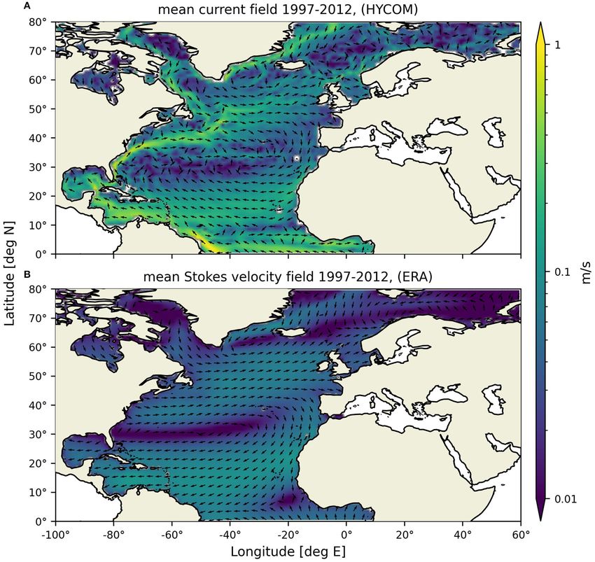
Bosi et al.                                                                                                              Stokes Drift and Particle Dispersal

water column is at the surface, where it is subject to the effect of          where C0 is the surface concentration, ν is a constant eddy
winds, currents, and waves (Reisser et al., 2015). One particular             diffusivity and wr is the particles’ rising speed, i.e. the speed at
wave effect that is prevalent close to the free surface is the Stokes         which particles rise due to buoyancy forces. From Equation (2),
drift. It is defined in Oceanography as the net drift that a particle         the vertical decay scale of particle concentration δp is inversely
moving in a fluid experiences in the direction of propagation                 proportional to their rising speed:
of the fluid’s wave field (Van den Bremer and Breivik, 2017).
The Stokes drift velocity, uE St , is also commonly described as the                                              ν
                                                                                                           δp =      .                                  (3)
difference between the average Lagrangian velocity of the particle                                                wr
at a mean depth, uE Lag , and the Eulerian velocity of the fluid at the
same mean depth, uE Eu (Röhrs et al., 2012; Breivik et al., 2016):            A typical value for eddy diffusivity in the upper ocean is
                                                                              ν = 10−2 m2 s−1 (Talley, 2011), while wr varies significantly
                              uE Lag = uE Eu + uE St .             (1)        depending on the chemical and physical structure of the
                                                                              considered item. For instance, oil droplets have a typical rising
The Stokes current field generally has larger spatial scales than             speed of 400 m day−1 (Drivdal et al., 2014), yielding a depth scale
the Eulerian velocity field and it has been shown to affect the               of about 2 m, while Arctic cod eggs with wr = 100 m day−1
transport of floating objects such as oil droplets (Drivdal et al.,           would lead to δp = 8.5 m. Marine litter items, such as small wood
2014), pelagic eggs and larvae (Röhrs et al., 2014), and plastic              pieces or plastic fragments with length scales of 1−10 cm, have an
(Onink et al., 2019).                                                         estimated upward terminal velocity of 0.1 to 1 ms−1 (Hinata et al.,
    The marine debris problem has been defined as a source,                   2017). The particle depth scale δp would then range between 10
pathway and sink issue (Hardesty et al., 2017). Two major                     and 1 cm. The Stokes drift on a rotating plane is counteracted by a
physical sinks of plastic pollution in the ocean are beaching at the          Eulerian return flow which dominates at depth, while the Stokes
coast and sinking to the bottom sediment (Kaandorp et al., 2020).             current is strongest at the surface (Van den Bremer and Breivik,
This study aims at investigating the timescales of the beaching               2017). For a single wave frequency, the Stokes drift decreases
process of floating particles and the main accumulation zones in              exponentially with depth. Its vertical scale for a full wave field,
the presence of Stokes drift, building directly onto existing work            δSt , has been estimated to be around 1.8 m for basins larger than
(see e.g., Iwasaki et al., 2017; Onink et al., 2019). The hypothesis          the gulf of Mexico (Clarke and Van Gorder, 2018). This depth is
is that particles at the ocean surface will disperse and gather               at least one order of magnitude smaller than the estimated Ekman
at the coast at a faster rate if Stokes drift is included in the              depth, δEk , in a large basin. Given the magnitude of the three
model. Coastal attractors are also expected to arise at different             depth scales, the following approximation for the ocean surface
locations as Stokes drift has been found to change the mean                   can be made:
direction of transport, e.g., steering particles toward the poles
(Onink et al., 2019). The hypothesis is tested by comparing two                                        δp < δSt < δEk .                                 (4)
Lagrangian particle tracking models (PTMs): one where particles
are advected by the Eulerian flow alone and one where Stokes                  The Lagrangian velocity experienced by particles under these
drift is included. Reanalysis data from the HYCOM ocean model                 conditions is equal to the sum of the Ekman and Stokes currents
(Eulerian current) and the ERA-interim wave model (Stokes                     (Clarke and Van Gorder, 2018) (see Appendix A for a more in
drift) are used to advect particles in the North Atlantic. The PTMs           depth derivation). PTM-REF then corresponds to the case where
are two-dimensional (no vertical axis). To justify this choice, a             δp > δSt and, conversely, PTM-SD corresponds to δp ≤ δSt .
theoretical background on the vertical scale of Stokes drift and
particle concentration is given in section 2.1. The model runs and
                                                                              2.2. The Particle Tracking Model
                                                                              To investigate how the inclusion of Stokes drift affects particle
the methods used for data processing are described in sections
                                                                              transport in a Lagrangian simulation, numerical experiments are
2.2 and 2.3. Section 3.1 presents an overview of the particle
                                                                              carried out with and without Stokes drift. For simplicity, the two
simulation output. The beaching process is analysed in terms of
                                                                              experiments will be hereon referred to as PTM-REF and PTM-SD
its timescales (section 3.2) and spatial patterns (section 3.3). The
                                                                              according to Table 1.
mean dispersal distance is calculated (section 3.4) and further
                                                                                  Daily means of eastward and northward water velocity from
forecasting of particle distribution over a longer time period is
                                                                              ocean model HYCOM are used to advect particles in PTM-
carried out (section 3.5). Finally, an interpretation of results and
                                                                              REF, called uEu and vEu , respectively. The HYCOM model (for
their implications on marine pollution is given in section 4.
                                                                              HYbrid Coordinate Ocean Model) is a data-assimilative hybrid
                                                                              isopycnal-sigma-pressure (generalised) coordinate ocean model
2. METHODS                                                                    (Chassignet et al., 2007). In PTM-SD, daily means of eastward
2.1. Particle Concentration                                                   and northward Stokes drift velocities, uSt and vSt , from wave
The present experiment focuses on the upper meter at the ocean                model ERA-Interim (Dee et al., 2011) are added to the HYCOM
surface, where the concentration of buoyant particles C is at                 velocity components. Both velocity datasets range from January
its maximum. For a steady state, C has a vertical distribution                1997 to December 2012 and cover the global ocean from 80◦ S
(Drivdal et al., 2014):                                                       to 80◦ N. The domain is reduced to the North Atlantic ocean
                                                wr
                                                                              between 100◦ W and 60◦ E and from the Equator up to the Arctic
                               C(z) = C0 ez     ν    ,             (2)        at 80◦ N. Conclusions regarding the North Atlantic can be applied

Frontiers in Marine Science | www.frontiersin.org                         2                                       August 2021 | Volume 8 | Article 697430
Bosi et al. Stokes Drift and Particle Dispersal
TABLE 1 | Velocity datasets and variables used for the two particle simulations, PTM-REF and PTM-SD.
Name of experiment Dataset(s) used Velocity components
PTM-REF HYCOM NCODA Global 1/12◦ Reanalysis (GLBu0.08/expt_19.1) u = uEu
v = vEu
PTM-SD HYCOM NCODA Global 1/12◦ Reanalysis (GLBu0.08/expt_19.1) u = uEu + uSt
ERA-interim Global 1/4◦ Reanalysis v = vEu + vSt
to the other ocean basins, where an equivalent structure in the where at least one particle was seeded at time t0 . Each active bin
accumulation of marine debris is observed (Maximenko et al., is identified by a unique number ranging from 0 to m−1, where m
2012). The initial condition consists of 2·104 particles distributed is the total number of active bins. The resulting five matrices are
randomly over the spatial domain. This initial condition is then averaged to produce the stochastic matrix Pij , also known
repeated five times, by releasing a batch of 2 · 104 particles on as a dispersal matrix (Botsford et al., 2009). Seasonal variability
January 1st of years 1997–2001, achieving a total of 105 particles. is thus captured in the dispersal matrix by mixing statistics from
The five batches are then synced so that all particles begin drifting different years. This computation is carried out for both PTM-
at the same time (t = 0) and a potential bias due to inter- REF and PTM-SD with 1t = 1 year, to compute mean dispersal
annual variability is avoided. Seeding particles for the first 5 years distance (or “MDD”), and with 1t = 10 years to make long-
is a trade-off between releasing particles for as long as possible term predictions of particle dispersal. The MDD is calculated as
while obtaining a drift period of at least 10 years for all particles. (Jonsson et al., 2020):
The OceanParcels v2.0 framework with its 4th order Runge-
Kutta advection scheme is used to advect particles (Delandmeter m
X
and Van Sebille, 2019). The particle simulations produce daily (MDD)i = Pij Qij , (6)
outputs which are then processed in the following ways. Firstly, j
the North Atlantic domain is gridded in 2◦ × 2◦ boxes. Southern
and northern boundaries are posed at 80◦ N and at the Equator, where Qij is a matrix of geographical distance between each
respectively. Finally, particles whose velocity drops to 10−7 ms−1 bin i and all other bins j. The MDD computed as in Equation
or less are considered beached and removed. This is based on the (6) indicates how far from their initial position particles are
numerical assumption that such particle velocity values would likely to be found after the time interval 1t. Long-term
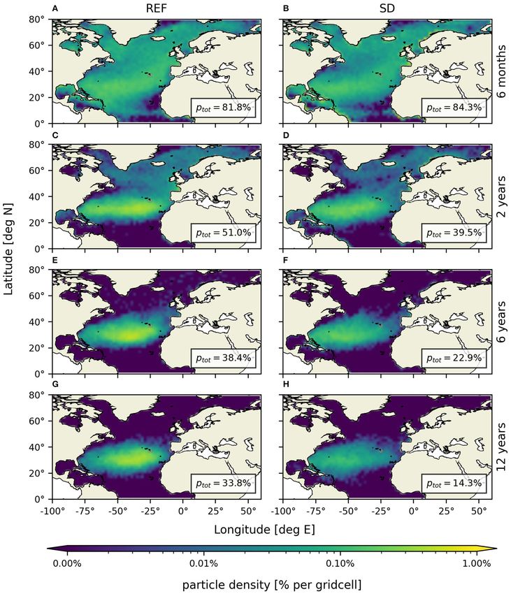
only appear on land cells. The time-averaged Eulerian and Stokes predictions of particle distribution are also computed using
drift velocities are shown in Figure 1 to gauge the main features matrix multiplication (Botsford et al., 2009). In particular, the
of the two. The maximum time-averaged Eulerian flow is one same initial condition used for PTM-REF is reshaped into a
order of magnitude faster than the time-averaged Stokes velocity, vector of size m, called here D(0) j . This is the distribution of
with peaks along the western boundaries given by the North particles at time t0 . Note that m is the number of 2◦ × 2◦ bins
Equatorial current and the Gulf stream, as well as the Caribbean that make up the domain, as in section 2.2. As powers of a
and Guiana currents (Figure 1A). The North Atlantic subtropical stochastic matrix are also stochastic matrices, it is possible to take
and subpolar gyres are easily identifiable: the former revolving (Pij )n to obtain predictions for the time interval n1t. The particle
anticyclonically between 10 and 50◦ N, and the latter rotating distribution at time t1 = n1t, called D(n)i , is then given by:
cyclonically in the Northern sector of the domain. The direction
of the Stokes drift velocity (Figure 1B) around the subtropical
gyre is consistent with large-scale atmospheric circulation (Trade D(n) n (0)
i = (Pij ) Dj . (7)
Winds and Westerlies). The effect of the Polar Easterlies is also
visible between 60 and 80◦ N along the coast of Greenland. Predictions obtained with the dispersal matrix are validated by
comparison with the model output. Figure 2 shows the resulting
2.3. Connectivity and Dispersal Distance anomaly. The matrix predictions overestimate concentrations
Adjacency matrices are a powerful tool to extract statistics on the in the subtropical accumulation zone compared to the model,
connectivity of different locations within the domain of a given especially in PTM-REF (dark red regions in Figures 2C–F). The
problem (Jonsson et al., 2020). Here, weighted adjacency matrices maximum discrepancy for PTM-REF in the subtropical region
are calculated for each of the five batches of particles. Each entry reaches 0.4% of particles per grid-cell, 0.2% more than in PTM-
pij of such matrices represents the probability of a particle seeded SD. Underestimation occurs, on the other hand, in almost all
in a bin i to be found in another bin j after a given time interval coastal bins, indicated by the blue lining along the land boundary.
1t. This is calculated as: In particular, the matrix prediction inaccurately represents the
ni→j concentration of particles along the coast of Central and South
pij = , (5) America, especially in PTM-SD, as well as the western coast of
ni
Europe and the southern coast of west Africa (Figures 2E,F).
where ni→j is the number of particles seeded in bin i and found The magnitude of the discrepancies increases over time as higher
in bin j at time t1 = 1t and ni is the number of particles in powers of the matrix are taken (low anomaly in Figures 2A,B).
bin i at time t0 = 0. Only active bins are considered, i.e., bins Nonetheless, the matrix and model outputs are overall in good
Frontiers in Marine Science | www.frontiersin.org 3 August 2021 | Volume 8 | Article 697430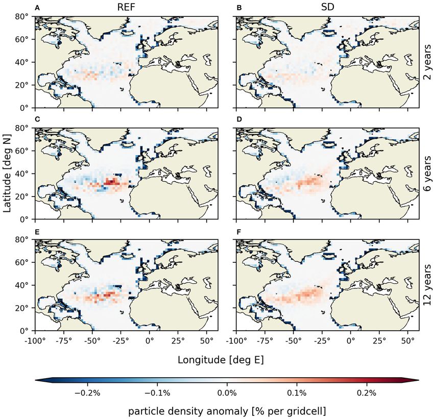
Bosi et al.                                                                                                                        Stokes Drift and Particle Dispersal

  FIGURE 1 | Current and Stokes drift velocities in the North Atlantic from global reanalysis ocean and wave models, HYCOM (A) and ERA-Interim (B), averaged over
  years 1997–2012. Note the logarithmic colour-scale.

agreement with each other, with a mean anomaly of O(0.04%) of                        have drifted away from this region. A similar divergence is
particles per grid-cell for both PTM-REF and PTM-SD.                                 also apparent at the Arctic boundary east of Greenland, as well
                                                                                     as in the Gulf of Mexico and Caribbean Sea. After 2 years
3. RESULTS                                                                           of run time (Figures 3C,D), the formation of a subtropical
                                                                                     accumulation zone around 30◦ N becomes visible, as observed in
3.1. An Overview of the PTMs                                                         previous studies (Maximenko et al., 2012). The area between this
Snapshots of the two particle tracking model runs are displayed                      subtropical patch and the Equator has been entirely cleared of
in Figure 3 to gain a qualitative view of the particle’s behaviour                   particles. A similar process appears after 6 years (Figures 3E,F),
over time and highlight the differences that arise when Stokes                       where the region North of the subtropical patch up to the Arctic
drift is included. The results suggest that there are areas of                       shows 0 concentration everywhere. The maximum concentration
particle convergence and areas of particle divergence. After 6                       in the subtropical patch decreases over time in PTM-SD while
months (Figures 3A,B), all particles seeded North of the Equator                     it remains stable in PTM-REF. At the end of the 12-year

Frontiers in Marine Science | www.frontiersin.org                                4                                          August 2021 | Volume 8 | Article 697430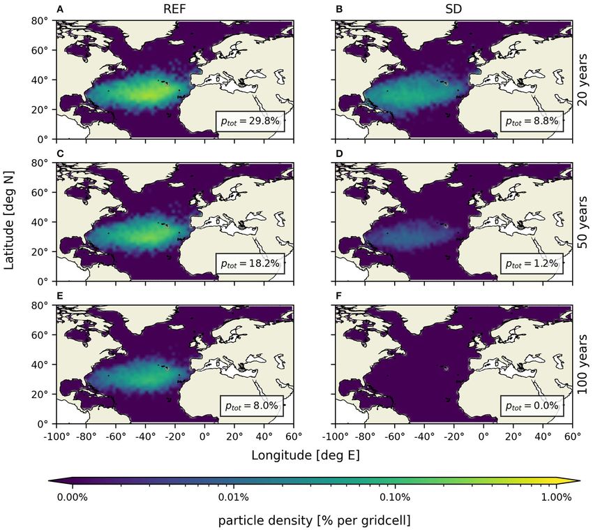
Bosi et al.                                                                                                                              Stokes Drift and Particle Dispersal

  FIGURE 2 | Anomaly between matrix and model predictions (= matrix - model). The adjacency matrix is calculated with a 1t of 1 year and predictions are calculated
  from the same initial condition as the PTMs. Colours represent the difference in particle concentration per 2◦ × 2◦ bin, in percentage, relative to the total number of
  particles. The anomaly is shown at snapshots of 2, 6, and 12 years for both PTM-REF (A,C,E) and PTM-SD (B,D,F).

run (Figures 3G,H), all remaining particles (i.e., particles that                        3.2. Beaching Timescales
have not beached) are in the accumulation zone. Overall,                                 Not enough clarity has yet been made on the residence time of
particle convergence/divergence occurs in the same areas in                              plastic pollution in the ocean, with estimations ranging from a
PTM-REF and PTM-SD. However, the timescales of dispersal                                 few years to millennia before it sinks to the bottom or it is washed
from the subtropical accumulation zone differ. In particular,                            ashore (Morét-Ferguson et al., 2010). The present experiment
concentrations decrease over time at a faster rate in PTM-                               provides some insight on the timescales of particle dispersal from
SD in this region. Just over 14% of particles are left in the                            the oceanic accumulation zone. The beaching test described in
domain by the end of the PTM-SD run, compared to almost 34%                              section 2.2 is applied to the PTM-REF and PTM-SD cases. The
in PTM-REF.                                                                              resulting amount of beached particles is shown, in percentage,

Frontiers in Marine Science | www.frontiersin.org                                    5                                            August 2021 | Volume 8 | Article 697430
Bosi et al.                                                                                                                            Stokes Drift and Particle Dispersal

  FIGURE 3 | Snapshots of model outputs after 6 months (A,B), 2 years (C,D), 6 years (E,F), and 12 years (G,H). Colours represent the amount of particles per 2◦ bin
  in percentage, relative to the number of seeded particles. Note the logarithmic scale in the colourbar. Beached particles are detected as in section 2.2 and removed.
  The text box indicates the amount of remaining particles, ptot .

Frontiers in Marine Science | www.frontiersin.org                                   6                                           August 2021 | Volume 8 | Article 697430
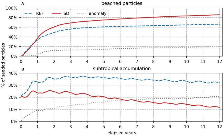
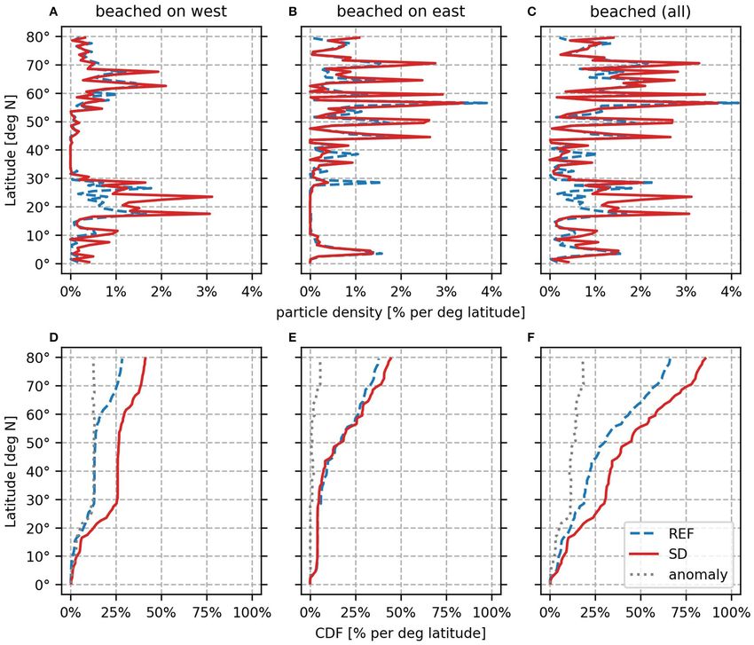
Bosi et al.                                                                                                                            Stokes Drift and Particle Dispersal

  FIGURE 4 | Amount of beached particles over time (A) and of particles located within the subtropical accumulation zone (B). Quantities are shown in percentage
  relative to the total number of particles seeded. Beached particles are detected as described in section 2.2. The subtropical accumulation zone is defined as a box
  with longitude between 70 and 18◦ W and latitude between 21 and 42◦ N. Data points are taken every 30 days.

in Figure 4A, while Figure 4B depicts the concentration in                              amount found in PTM-SD. The oscillation in Figure 4B appears
the subtropical accumulation zone. The coastal accumulation                             as a result of seasonal variability.
increases rapidly within the first 2 years and it continues growing,
albeit with a smaller gradient, until the end of the run. After 12                      3.3. Spatial Differences
years, 86% of particles seeded in PTM-SD have beached; 20%                              Discrepancies in the beaching process emerge not only in terms
more than in PTM-REF. New particles are seeded annually over                            of timescales, but also as far as the main coastal areas attracting
the entire domain for the first 5 years. Some of these particles are                    particles. It is thus worth looking at their distribution at the
located, at time 0, in those areas of divergence seen in Section. 3.1.                  end of the run on each side of the domain, east and west
The extreme increase in the number of beached particles in the                          (see Figure 5). Figures 5A,B show the meridional distribution
Figure 4A reflects the quick removal of particles from divergence                       of beached particles on each side of the domain as a sum in
areas. As these regions empty out, the beaching process slows                           the longitudinal direction of the amount of particles per square
down. The average annual beaching rate (excluding the 5 years                           degree. Figure 5C depicts the same distribution for all beached
of seeding) is 1.6% in PTM-SD. This rate is halved in PTM-REF                           particles. Percentages are calculated from the total amount of
(0.8%). When particles are seeded, about 22% of particles are                           particles. From the top panels, it is clear that PTM-REF (blue
located in the offshore accumulation zone. The concentration                            dashed line) and PTM-SD (red line) have a similar distribution in
in this subtropical patch increases within the first 4–5 years,                         the meridional direction. In particular, they present maxima and
partly due to the constant addition of particles during this time,                      minima at similar latitudes. No particles are found anywhere on
reaching a maximum of 37% of particles in PTM-REF and 25% in                            the coast of the US between 33 and 45◦ N (Figure 5A) and on the
PTM-SD. After the first 3–5 years, it then decreases steadily with                      coast of west Africa between 10 and 27◦ N (Figure 5B). Particles
a stronger gradient in PTM-SD. The anomaly between the two                              are located mainly North of 30◦ N in the east, while they appear
experiments increases over time, indicating that the subtropical                        split in half between north and south in the west. To gain a better
gyre is a stronger attractor without the influence of Stokes drift                      understanding of the north-south distribution, the cumulative
(PTM-REF case). In particular, the subtropical box contains 32%                         distribution function (CDF) is shown in the bottom panels
of particles in PTM-REF at the end of the run, 20% more than the                        (Figures 5D–F). It is calculated by integrating the meridional

Frontiers in Marine Science | www.frontiersin.org                                   7                                            August 2021 | Volume 8 | Article 697430
Bosi et al.                                                                                                                              Stokes Drift and Particle Dispersal

  FIGURE 5 | The top panels show the meridional distribution of beached particles at the end of the run on the western side of the domain (A), on the eastern side (B),
  as well as for all beached particles (C). Data points are in 1◦ bins and result from a sum in the longitudinal direction. The bottom panels depict the cumulative
  distribution function (or “CDF”) obtained by integrating the particle distribution from South to North. This is shown for particles beached on either side of the domain
  (D,E) and for all beached particles (F). Percentages are calculated out of the total number of particles seeded.

distribution of beached particles from south to north. The total                         coast South of 30◦ N (Figure 5E). This corresponds to a peak in
number of beached particles is around 20% higher in PTM-SD                               the southern coast of West Africa. The vast majority of particles
(Figure 5F), in line with section 4. Half of the total beached                           on the eastern side of the North Atlantic beaches on the European
particles are located in the northern region North of 55◦ N. This                        coast North of 35◦ N, from Gibraltar to Ireland and Scotland,
zonal threshold is not maintained when the CDF is calculated                             up to the entire coast of Norway and Svalbard. This amounts to
separately for the eastern and western coastal boundaries. In                            around 30% of all particles in PTM-REF and 40% in PTM-SD.
PTM-REF over 13% of particles end up South of 30◦ N on                                   The highest peak in concentration of beached particles is found
the western side of the North Atlantic (Figure 5D). This value                           in Northern Ireland in both experiments.
reaches 25% in PTM-SD, meaning that a fourth of all particles
beaches on the coast of Central America in this configuration.                           3.4. Mean Dispersal Distance
Another 14% of particles is found along the boundary North of                            Mean dispersal distance (MDD) calculated as in section 2.3 is
55◦ N in both PTMs. This covers the coasts of Canada, Greenland                          shown in Figure 6. Low MDD (close to 0 km) is found within
and Iceland. Conversely,
Bosi et al.                                                                                                                         Stokes Drift and Particle Dispersal

  FIGURE 6 | Mean yearly dispersal distance, in km, for PTM-REF (A) and PTM-SD (B) calculated using Pij with a 1t of 1 year, as in section 2.3. The bottom panel (C)
  shows the anomaly between the two experiments (= MDDSD − MDDREF ). The star markers represent the maximum value in each figure.

Frontiers in Marine Science | www.frontiersin.org                                 9                                           August 2021 | Volume 8 | Article 697430
Bosi et al.                                                                                                           Stokes Drift and Particle Dispersal

regions of West Africa, Northern Europe, and the Caribbean.                  4. DISCUSSION
A significant amount of particles was found to beach in these
regions (see section 3.3). Particles seeded in any of these locations        4.1. Interpretation of Results
are likely to be in the same position after a year. The sector               The motivation behind the present study was the hypothesis that
corresponding to the centre of the subtropical accumulation zone             the inclusion of Stokes drift in models investigating trajectories
showing low MDD is larger in PTM-REF (Figure 6A) than in                     of floating objects is of particular importance, as implied by
PTM-SD (Figure 6B), suggesting that particles are more likely to             previous analyses (Drivdal et al., 2014; Onink et al., 2019). This
leave the gyre within a year if Stokes drift is included in the PTM.         hypothesis is hereby confirmed as Stokes drift is seen to have an
The highest values of MDD surround this area, following the                  impact both on the timescales of particle dispersal and on the
anticyclonic circulation in the North Atlantic. From the anomaly             concentration in the main convergence zones. An accumulation
plot (Figure 6C), it can be noted that MDD in the PTM-SD                     zone centred at 30◦ N is observed within the first 2 years of run-
case exceeds PTM-REF almost everywhere, with the maximum                     time in both PTMs, covering the subtropical gyre. An equivalent
difference found by the Canary islands (star marker). However,               aggregation of particles in the subtropics has been found in
the mean dispersal distance in PTM-REF is larger along the                   a variety of modelling experiments (Lebreton et al., 2012), as
strong Guiana and Caribbean currents. Stokes drift is weak here              well as from trajectories of satellite-tracked Lagrangian drifters
(see Figure 1) and pushes directly toward the coast, explaining              (Maximenko et al., 2012) and in-situ observations (Morét-
why particles initialised here in PTM-SD are not likely to travel            Ferguson et al., 2010). Similar build-ups appear in the subtropics
far. An area of negative anomaly is also found within the subpolar           in all five ocean basins as a result of Ekman convergence (Onink
gyre. Here, Stokes drift is strongly directed toward the Norwegian           et al., 2019). The distribution of beached particles at the end of
coast, promoting beaching, while the Eulerian current points                 the PTM runs reveals that the most affected coastal areas are
away from it. The maximum dispersal distance is located near                 northern Europe on the eastern side of the North Atlantic and
the Equatorial current at 30◦ W in the PTM-REF case. In PTM-                 Central/South America on the western side. This is in line with
SD, however, it is observed right off the coast of west Africa at            the direction of large-scale atmospheric circulation: particles are
20◦ N, coinciding with the Canary current. The maximum MDD                   pushed southwest-ward by the Trade Winds and northeast-ward
in PTM-SD is well over a thousand kilometers larger than in                  by the Westerlies. From the mean dispersal distance calculation
PTM-REF. At 20◦ N, the distance between the African continent                (section 3.4), it can be inferred that particles released near the
(20◦ W) and the islands in Central America (60◦ W) is around                 European coast are likely to beach locally. This is in agreement
4,200 km. This suggests that a particle seeded in this area may              with previous studies where the densely populated north-east
cross the North Atlantic ocean in less than a year’s time if Stokes          Atlantic region turned out to be highly impacted by beaching
drift is taken into consideration.                                           and coastal retention (Chenillat et al., 2021). On the other hand,
                                                                             small islands in Central America may be particularly affected
                                                                             by nonnative marine litter. These islands are located at the rim
3.5. Matrix Predictions                                                      of the subtropical accumulation zone, from which they receive
The calculation of an adjacency matrix allows for predictions that           a constant leakage of particles which may be originating from
go beyond the 12 years of the model run and require minimal                  the other side of the Atlantic and travelling across the ocean in
computational time. With this goal, matrix Pij is computed for               less than a year (Lachmann et al., 2017). The increased mean
PTM-REF and PTM-SD with 1t = 10 years. This allows to                        dispersal distance in PTM-SD may occur as a result of the method
investigate particle distribution on a timescale of decades. It is           chosen to include Stokes drift in the model. As the Stokes drift
worth pointing out that this calculation is valid for any initial            here is linearly added to the Eulerian flow, the velocity advecting
condition. The calculation in Equation (7) is carried out using              particles in PTM-SD is always larger in magnitude than in PTM-
(Pij )n with n = 2, 5, 10 using the same initial condition as                REF, causing particles to travel faster. However, the consistency
PTM-REF. The resulting distributions are shown in Figure 7.                  in direction of the Stokes drift and its predominantly zonal
Previously made observations on the location of divergence                   pattern suggest that such an increment in MDD is plausible.
and convergence zones still apply over a longer timescale. In                The adjacency matrix predictions compare well with the model
particular, non-zero concentrations are observed only within the             results (Figure 2). Despite the coarse resolution of Pij , it succeeds
subtropical accumulation zone. The garbage patch at 30◦ N is                 in adequately representing the formation of the North Atlantic
present in both cases and in all snapshots, albeit with varying              garbage patch and its decay over time. The long-term prediction
concentrations. After 20 years (Figures 7A,B), 28.3% of particles            (Figure 7) confirms that Stokes drift increases the rate of particle
are still floating at the ocean surface in PTM-REF. In PTM-SD,               dispersal in the subtropical accumulation zone over time. The
on the other hand, only 8.4% of all particles remain in the ocean            Stokes velocity measured by Lagrangian surface drifters has been
after 20 years: around 20% less than in the case without Stokes              shown to reach a comparable magnitude to the Eulerian current
drift. This anomaly agrees with the findings in sections 3.2 and             measured by ADCPs during strong wind events. However, under
3.3. Fifty years after initialisation (Figures 7C,D), the amount of          normal conditions, its magnitude decreases to only 20% of the
active particles has decreased by over 10% in PTM-REF and by                 Eulerian current on average (Röhrs et al., 2012). Despite this
7% in PTM-SD, reaching only 1.1%. All particles have beached                 seemingly small contribution to the total current, the Stokes drift
after 100 years in PTM-SD, while almost 8% of the initial amount             has a non-negligible effect on the rate of dispersal of floating
remain active in PTM-REF (Figures 7E,F).                                     particles. We find that the number of beached particles per year

Frontiers in Marine Science | www.frontiersin.org                       10                                      August 2021 | Volume 8 | Article 697430
Bosi et al. Stokes Drift and Particle Dispersal
FIGURE 7 | Adjacency matrix predictions after 20 (A,B), 50 (C,D), and 100 years (E,F). Pij is calculated with 1t = 10 years to match the timescale of the prediction.
Note the logarithmic scale in the colourbar.
is doubled in PTM-SD compared to PTM-REF (section 3.2). particles. The residence time at the surface before sinking due to
Evidence of this was previously given in Onink et al. (2019), biofouling is estimated in Chubarenko et al. (2016) for different
where Stokes drift was shown to counteract the formation of types of micro-plastic particles. The study finds that polyethylene
garbage patches resulting from Ekman convergence. fibres spend 6–8 months within the upper layers, while spherical
particles and plastic pieces remain at the surface for up to 10–15
4.2. Areas of Improvement for the PTM years. In the latter case, the inclusion of sinking in the present
The present simulation succeeds in capturing the effects of model would not significantly affect the result, as the timescale of
large-scale phenomena acting on particle transport under the sinking is larger than the total run time and estimated residence
chosen conditions, in particular the formation of convergence time. However, in the case of polyethylene fibres or—more
and divergence zones. However, the model does not account generally—of objects whose sinking rate is comparable to the
for (1) the sinking of particles to the ocean bottom and (2) beaching rate or faster, the inclusion of a sinking flux in the
the possibility for particles that have washed ashore to drift model would be of great importance. In future work, a more
back into the ocean, thus overestimating the amount of beached realistic budget of particle density should be employed with the
Frontiers in Marine Science | www.frontiersin.org 11 August 2021 | Volume 8 | Article 697430Bosi et al. Stokes Drift and Particle Dispersal
inclusion of a flux transporting particles from the surface to within the water column and eventually sink, while larger—
the ocean bottom. In the framework of adjacency matrices, this or in general, more buoyant—objects are more likely to be
can be represented by the probability psrf →btm of transitioning transported by winds and currents to one of the convergence
from the surface to the ocean bottom during a time interval 1t zones, whether it be the coast or the subtropical garbage patch.
(Liubartseva et al., 2018): As seen in section 2.1, the Stokes drift has its maximum at the
ocean surface. The Lagrangian velocity of highly buoyant items at
τage
−T the ocean surface is equal to the sum of the Eulerian velocity and
psrf →btm = s(1 − e surf ), (8) the Stokes drift velocity (Equation A5, Clarke and Van Gorder,
2018). If these objects are located just below the surface, where
where s is the rate of sedimentation, τage is the particle’s age and they are not directly affected by winds, their behaviour is then
Tsurf is its residence time at the ocean surface. Note that the closely described by the PTM-SD configuration of the model.
probability of sinking increases exponentially with the particle’s Nevertheless, the PTM-REF case is not unrealistic. As seen in
age, giving a realistic representation of the weathering of marine section 2.1, the Stokes drift is counteracted by an Eulerian return
debris at the surface and the consequent buoyancy loss. In flow which prevails below the Stokes depth δSt . The return flow is
terms of beaching, a strict boundary condition at the coast not present at the ocean surface and was thus not accounted for
was chosen: particles reaching a land-cell and a certain velocity in PTM-SD (Equation A5). However, if the depth scale of particle
(< 10−7 ms−1 ) are considered beached and erased. Beaching concentration, δp , were larger than δSt , the effect of the Stokes
is thus an irreversible process in the PTMs. This is however drift on particle transport would be increasingly dampened by
not necessarily realistic. Items of marine litter that have washed the Eulerian return flow as depth increases. This would lead to a
ashore may in fact drift back into the ocean as a consequence scenario that is closer to PTM-REF. A similar result was derived
of e.g., a change in wind direction or strong wave action at in Iwasaki et al. (2017), where the contribution of Stokes drift
the coast. With that in mind, a less rigid boundary condition to particle motion was found to depend on particle size, with
was tested in previous runs of the PTMs, where beaching was buoyant large particles moving more rapidly at the surface.
reversible. In this configuration, particles whose velocity became
smaller than 10−7 ms−1 were counted as “beached” but not
erased, allowing them to drift back into the flow. The annual 5. CONCLUSION
rate of dispersal from the subtropical accumulation zone and
onto the coast remained doubled in PTM-SD compared to PTM- This work presents a comparison between two different particle
REF. A seasonal pattern was discovered in PTM-SD with a tracking models (PTMs) to shed light on the effect of Stokes
higher number of beached particles in summer and a decrease in drift on the dispersal of floating objects at the ocean surface.
winter. The same oscillation was not observed in PTM-REF and In the first experiment (PTM-REF) particles are advected by
is likely due to a change in wind direction affecting the Stokes the Eulerian current alone, while in the second (PTM-SD)
drift. However, there is no indication that the way the model the Stokes drift is added linearly to the Eulerian current to
represented this flux in and out of coastal bins is realistic and transport particles. Global renalysis products HYCOM and ERA-
was thus neglected here. As a future improvement to the PTM, interim are used for the Eulerian velocity and Stokes drift,
a horizontal diffusivity term such as the one used in e.g., Iwasaki respectively. Particles are seeded with a random geographical
et al. (2017) would have to be included to obtain a more realistic distribution over the North Atlantic and at different times to
image of the beaching process. avert biases caused by inter-annual variability. The results reveal
areas of particle convergence both within the basin and along
4.3. Application to Marine Plastic the coast. An offshore accumulation of particles develops in
Plastic debris in the ocean has two main sinks: the coast and the subtropics, around 30◦ N. This is observed in all five ocean
the bottom sediment (Kaandorp et al., 2020). The buoyancy of basins and has been referred to in the literature as a “garbage
an object highly influences its fate, determining which of the patch.” The PTMs and adjacency matrix predictions show that
two sinks it will end up in. Buoyancy depends on chemical the garbage patch disperses particles faster in PTM-SD, with
composition and physical properties, such as size and shape. an annual beaching rate that is doubled compared to the one
Plastic objects at the ocean surface are subject to weathering in PTM-REF. The coastal environment is highly affected as it
due to UV radiation as well as temperature and salinity changes becomes a stronger attractor for floating particles than the open
(Jahnke et al., 2017). Weathering leads to fragmentation, which ocean. The model suggests Western Europe and Central America
is the process of larger objects breaking up into smaller pieces, are the coastal regions most affected by beaching of particles.
leading to the formation of “secondary microplastic” (Jahnke However, due to enormous difficulties in sampling plastic debris
et al., 2017). The rate at which microplastics sink to the bottom in the ocean, it is difficult to validate these results against
sediment is inversely proportional to their characteristic length- independent information. It is shown by the mean dispersal
scale: given the same buoyancy, the smaller the object, the faster distance calculation that particles beaching in Central America,
it sinks (Chubarenko et al., 2016). Sinking happens mainly as which is located at the edge of the subtropical gyre, may originate
a consequence of biofouling, as the growth of biofilm around from all the way across the ocean. Particles released off the
plastic objects is found to increase their density (Jahnke et al., coast of West Africa in PTM-SD, where the MDD is at its
2017). This suggests that microplastics are more likely to settle maximum, take under a year to be found almost 6,000 km
Frontiers in Marine Science | www.frontiersin.org 12 August 2021 | Volume 8 | Article 697430Bosi et al. Stokes Drift and Particle Dispersal
from their starting point. On the other hand, particles found dampened by the Eulerian return flow. Under these assumptions,
stuck on the European coast are likely domestic. Investigating both PTMs are deemed valid descriptors of two different limit
the connectivity of different regions of an oceanic basin gives cases: PTM-REF applies to the case where the depth scale of
insight on the distances travelled by particles and their timescales. particle concentration is larger than the Stokes depth (δp > δSt ),
Such considerations can be useful in informing policy change while PTM-SD better reflects the case where particles concentrate
on marine pollution prevention and clean-up. It is estimated at the very surface of the ocean (δp ≤ δSt ).
that 60–80% of marine debris is comprised of plastic (Lebreton
et al., 2012). The present results suggest that the idea that marine DATA AVAILABILITY STATEMENT
plastic may spend hundreds of years floating in the open ocean
is likely a misconception. We highlight the need to take into The raw data supporting the conclusions of this article will be
account the Stokes drift velocity when modelling the transport of made available by the authors, without undue reservation.
marine debris by showing that ignoring this wave effect may be
causing an overestimation of the residence time of particles in the AUTHOR CONTRIBUTIONS
subtropical accumulation zones. This is of particular importance
when modelling the behaviour of buoyant objects of marine litter All authors contributed to conception and design of the study.
that sit just below the surface, where the Stokes drift is at its SB performed the numerical simulation, statistical analysis, and
maximum. On the other hand, for debris that tends to settle lower wrote the manuscript, with support from GB and FR. GB and FR
in the water column (such as certain items of microplastic, Hinata supervised the findings of this work. All authors contributed to
et al., 2017), the effect of Stokes drift on particle transport is manuscript revision, read, and approved the submitted version.
REFERENCES microplastics based on the population decay of tagged meso-and macrolitter.
Mar. Pollut. Bull. 122, 17–26. doi: 10.1016/j.marpolbul.2017.05.012
Botsford, L., White, J. W., Coffroth, M.-A., Paris, C., Planes, S., Shearer, T., et al. Iwasaki, S., Isobe, A., Kako, S., Uchida, K., and Tokai, T. (2017). Fate of
(2009). Connectivity and resilience of coral reef metapopulations in marine microplastics and mesoplastics carried by surface currents and wind waves: a
protected areas: matching empirical efforts to predictive needs. Coral Reefs 28, numerical model approach in the sea of Japan. Mar. Pollut. Bull. 121, 85–96.
327–337. doi: 10.1007/s00338-009-0466-z doi: 10.1016/j.marpolbul.2017.05.057
Breivik, Ø., Bidlot, J.-R., and Janssen, P. A. (2016). A stokes drift Jahnke, A., Arp, H. P. H., Escher, B. I., Gewert, B., Gorokhova, E., Kühnel, D., et al.
approximation based on the phillips spectrum. Ocean Model. 100, 49–56. (2017). Reducing uncertainty and confronting ignorance about the possible
doi: 10.1016/j.ocemod.2016.01.005 impacts of weathering plastic in the marine environment. Environ. Sci. Technol.
Chassignet, E. P., Hurlburt, H. E., Smedstad, O. M., Halliwell, G. R., Hogan, P. J., Lett. 4, 85–90. doi: 10.1021/acs.estlett.7b00008
Wallcraft, A. J., et al. (2007). The hycom (hybrid coordinate ocean model) data Jonsson, P. R., Moksnes, P.-O., Corell, H., Bonsdorff, E., and Nilsson Jacobi, M.
assimilative system. J. Mar. Syst. 65, 60–83. doi: 10.1016/j.jmarsys.2005.09.016 (2020). Ecological coherence of marine protected areas: new tools applied to
Chenillat, F., Huck, T., Maes, C., Grima, N., and Blanke, B. (2021). Fate of floating the Baltic sea network. Aquat. Conserv. Mar. Freshw. Ecosyst. 30, 743–760.
plastic debris released along the coasts in a global ocean model. Mar. Pollut. doi: 10.1002/aqc.3286
Bull. 165:112116. doi: 10.1016/j.marpolbul.2021.112116 Kaandorp, M. L., Dijkstra, H. A., and van Sebille, E. (2020). Closing the
Chubarenko, I., Bagaev, A., Zobkov, M., and Esiukova, E. (2016). On some physical mediterranean marine floating plastic mass budget: inverse modeling of
and dynamical properties of microplastic particles in marine environment. sources and sinks. Environ. Sci. Technol. 54, 11980–11989. doi: 10.1021/acs.est.
Mar. Pollut. Bull. 108, 105–112. doi: 10.1016/j.marpolbul.2016.04.048 0c01984
Clarke, A. J., and Van Gorder, S. (2018). The relationship of near-surface Lachmann, F., Almroth, B. C., Baumann, H., Broström, G., Corvellec, H.,
flow, stokes drift and the wind stress. J. Geophys. Res. 123, 4680–4692. Gipperth, L., et al. (2017). Marine plastic litter on small island developing states
doi: 10.1029/2018JC014102 (SIDS): impacts and measures. Report No. 2017:4. Swedish Institute for the
Dee, D. P., Uppala, S. M., Simmons, A., Berrisford, P., Poli, P., Kobayashi, S., Marine Environment.
et al. (2011). The era-interim reanalysis: Configuration and performance of Lebreton, L.-M., Greer, S., and Borrero, J. C. (2012). Numerical modelling
the data assimilation system. Q. J. R. Meteorol. Soc. 137, 553–597. doi: 10.1002/ of floating debris in the world’s oceans. Mar. Pollut. Bull. 64, 653–661.
qj.828 doi: 10.1016/j.marpolbul.2011.10.027
Delandmeter, P., and Van Sebille, E. (2019). The parcels v2.0 lagrangian Liubartseva, S., Coppini, G., Lecci, R., and Clementi, E. (2018). Tracking plastics
framework: new field interpolation schemes. Geosci. Model Dev. 12, 3571–3584. in the mediterranean: 2d lagrangian model. Mar. Pollut. Bull. 129, 151–162.
doi: 10.5194/gmd-12-3571-2019 doi: 10.1016/j.marpolbul.2018.02.019
Drivdal, M., Broström, G., and Christensen, K. (2014). Wave-induced mixing and Maximenko, N., Hafner, J., and Niiler, P. (2012). Pathways of marine debris
transport of buoyant particles: application to the statfjord a oil spill. Ocean Sci. derived from trajectories of lagrangian drifters. Mar. Pollut. Bull. 65, 51–62.
10:977. doi: 10.5194/os-10-977-2014 doi: 10.1016/j.marpolbul.2011.04.016
Ebbesmeyer, C. C., and Ingraham, W. J. Jr. (1994). Pacific toy spill fuels ocean Morét-Ferguson, S., Law, K. L., Proskurowski, G., Murphy, E. K., Peacock, E.
current pathways research. Eos Trans. Am. Geophys. Union 75, 425–430. E., and Reddy, C. M. (2010). The size, mass, and composition of plastic
doi: 10.1029/94EO01056 debris in the western North Atlantic ocean. Mar. Pollut. Bull. 60, 1873–1878.
Hancock, L. (2019). Plastic in the ocean. Available online at: https://www. doi: 10.1016/j.marpolbul.2010.07.020
worldwildlife.org/magazine/issues/fall-2019/articles/plastic-in-the-ocean Onink, V., Wichmann, D., Delandmeter, P., and Van Sebille, E. (2019). The
(accessed August 2, 2021). role of Ekman currents, geostrophy, and stokes drift in the accumulation of
Hardesty, B. D., Harari, J., Isobe, A., Lebreton, L., Maximenko, N., Potemra, J., floating microplastic. J. Geophys. Res. 124, 1474–1490. doi: 10.1029/2018JC
et al. (2017). Using numerical model simulations to improve the understanding 014547
of micro-plastic distribution and pathways in the marine environment. Front. Reisser, J., Slat, B., Noble, K., Du Plessis, K., Epp, M., Proietti, M.,
Mar. Sci. 4:30. doi: 10.3389/fmars.2017.00030 et al. (2015). The vertical distribution of buoyant plastics at sea: an
Hinata, H., Mori, K., Ohno, K., Miyao, Y., and Kataoka, T. (2017). An estimation observational study in the North Atlantic gyre. Biogeosciences 12, 1249–1256.
of the average residence times and onshore-offshore diffusivities of beached doi: 10.5194/bg-12-1249-2015
Frontiers in Marine Science | www.frontiersin.org 13 August 2021 | Volume 8 | Article 697430Bosi et al. Stokes Drift and Particle Dispersal
Röhrs, J., Christensen, K. H., Hole, L. R., Broström, G., Drivdal, M., Conflict of Interest: The authors declare that the research was conducted in the
and Sundby, S. (2012). Observation-based evaluation of surface wave absence of any commercial or financial relationships that could be construed as a
effects on currents and trajectory forecasts. Ocean Dyn. 62, 1519–1533. potential conflict of interest.
doi: 10.1007/s10236-012-0576-y
Röhrs, J., Christensen, K. H., Vikebø, F., Sundby, S., Saetra, Ø., and Broström, G.
(2014). Wave-induced transport and vertical mixing of pelagic eggs and larvae. Publisher’s Note: All claims expressed in this article are solely those of the authors
Limnol. Oceanogr. 59, 1213–1227. doi: 10.4319/lo.2014.59.4.1213 and do not necessarily represent those of their affiliated organizations, or those of
Talley, L. D. (2011). Descriptive Physical Oceanography: An Introduction. London, the publisher, the editors and the reviewers. Any product that may be evaluated in
UK: Academic Press. doi: 10.1016/B978-0-7506-4552-2.10001-0
this article, or claim that may be made by its manufacturer, is not guaranteed or
Vallis, G. K. (2017). Atmospheric and Oceanic Fluid Dynamics. Cambridge, UK:
endorsed by the publisher.
Cambridge University Press. doi: 10.1017/9781107588417
Van den Bremer, T., and Breivik, Ø. (2017). Stokes drift. Philos. Trans. R. Soc. A
Math. Phys. Eng. Sci. 376:20170104. doi: 10.1098/rsta.2017.0104 Copyright © 2021 Bosi, Broström and Roquet. This is an open-access article
Weyler, R. (2017). The ocean plastic crisis: plastic debris appears in every ocean distributed under the terms of the Creative Commons Attribution License (CC BY).
of the world. Available online at: https://www.greenpeace.org/usa/the-ocean- The use, distribution or reproduction in other forums is permitted, provided the
plastic-crisis/ (accessed August 1, 2021). original author(s) and the copyright owner(s) are credited and that the original
Wijffels, S., Firing, E., and Bryden, H. (1994). Direct observations of the ekman publication in this journal is cited, in accordance with accepted academic practice.
balance at 10 n in the pacific. J. Phys. Oceanogr. 24, 1666–1679. doi: 10.1175/ No use, distribution or reproduction is permitted which does not comply with these
1520-0485(1994)0242.0.CO;2 terms.
Frontiers in Marine Science | www.frontiersin.org 14 August 2021 | Volume 8 | Article 697430Bosi et al. Stokes Drift and Particle Dispersal
2
A. APPENDIX A—THEORETICAL Ef × (EuEk + uE St ) = ν ∂ uE Ek , (A3)
BACKGROUND ∂z2
A.1. The Vertical Structure of Stokes Drift where Ef = f · kE is the constant Coriolis parameter f multiplied
For a single wave frequency ω of a surface gravity wave in a by the vertically directed unit vector kE and ν is a constant eddy
deep ocean, the Stokes drift has the following vertical profile viscosity. Note that, in the absence of friction or mixing, this
(Van den Bremer and Breivik, 2017): equation simply yields uE Ek = −EuSt . This implies that Stokes drift
has an induced counter current at a steady state in a rotating
uE St(ω) (z) = c(ak)2 e2kz Eewave , (A1) ocean. Recalling from standard Ekman theory that the Ekman
depth scale is:
where c is the phase speed of the wave, a its amplitude, k the wave s
number, z the fluid depth, negative downwards with z = 0 at 2ν
the surface, and Eewave the unit vector in the direction of wave δEk = (A4)
f
propagation. The Stokes vertical scale for a single wave frequency
δSt is then proportional to wavelength: long waves induce a and, using the vertical profile of uE St(ω) (z) for a single frequency
deeper Stokes drift. Using the dispersion relation for deep water given above, Equation (A3) can be solved analytically, giving the
surface gravity waves, ω2 = gk (Vallis, 2017), the vertical decay following complex solution:
scale becomes:
g τ0 (1 − i) (i+1)z
δSt = . (A2) ūEk (z) = e δEk
2ω2 ρ0 f δEk
In a realistic ocean, the wave field is composed of a sum of waves ūSt0 z
2 δSt
(i+1)
+ 2iε e − ε(i + 1)e δEk
z , (A5)
with different frequencies. To obtain a more truthful picture 1 − 2iε 2
of the vertical scale of the Stokes drift, Equation (A1) must
therefore be integrated over the whole wave spectrum S(ω). The where ū = u + iv is the complex notation for uE and the non-
Stokes depth δSt calculated from buoy measurements in different dimensional number ε has been introduced as the ratio between
locations in the Gulf of Mexico and North Pacific ocean is found the Stokes and the Ekman depths, ε = δδSt . The first term in
Ek
to range between 59 cm and 2 m. (Clarke and Van Gorder, 2018). Equation (A5) is the standard Ekman flow, obtained when there
is no surface Stokes drift. The second term represents what is
A.2. Wind-Driven Ekman Currents and known as the Stokes-induced Eulerian return flow. The mass
Return Flow transport due to Stokes drift is divergent on the scale of the
It is important to understand how the Stokes drift affects the wave group and acts to “pump” water from the waves’ trailing
equations of motion at the ocean surface. To do this, the classical edge to their leading edge (Van den Bremer and Breivik, 2017).
Ekman problem (Vallis, 2017) can be solved with the inclusion of It therefore generates an opposite Eulerian flow to balance it
the Coriolis-Stokes force: Ef × uE St (Van den Bremer and Breivik, out and maintain conservation of (vertically integrated) mass
2017). This force arises in the presence of Stokes drift in a rotating and momentum in the water column. For a deep enough ocean,
ocean. In the Northern Hemisphere, it is at right angles with the the Stokes drift prevails at the surface above the e-folding
direction of wave propagation and further deflects the Eulerian depth, while the return flow, which has a slower vertical decay,
current (Drivdal et al., 2014). During strong wind and high wave dominates far below the free surface (Breivik et al., 2016). The
events it has a comparable magnitude to that of the standard magnitude of uSt was found to range between 3 and 13 cm s−1
Coriolis force (Röhrs et al., 2012). For a steady state and in a (Clarke and Van Gorder, 2018), while the Ekman (ageostrophic)
deep ocean with no horizontal pressure gradients, the equation current velocity near the surface has been estimated to average 4
of motion becomes: ms−1 in the Atlantic ocean (Wijffels et al., 1994).
Frontiers in Marine Science | www.frontiersin.org 15 August 2021 | Volume 8 | Article 697430You can also read