A fast solver for a class of linear systems
←
→
Page content transcription
If your browser does not render page correctly, please read the page content below
A fast solver for a class of linear systems ∗
Ioannis Koutis Gary L. Miller Richard Peng
Computer Science Dept. Computer Science Dept. Computer Science Dept.
U. of Puerto Rico-Rio Piedras Carnegie Mellon University Carnegie Mellon University
ioannis.koutis@upr.edu glmiller@cs.cmu.edu yangp@cs.cmu.edu
ABSTRACT and their relationships as networks, also known as graphs,
The solution of linear systems is a problem of fundamental and use solvers to extract information from them. The
theoretical importance but also one with a myriad of appli- resulting linear systems frequently obey simple constraints
cations in numerical mathematics, engineering and science. which classifies them as symmetric diagonally dominant
Linear systems that are generated by real-world applications (SDD).
frequently fall into special classes. Recent research led to a An example of an area where such systems arise is in the
fast algorithm for solving symmetric diagonally dominant analysis of social networks. Such networks can be repre-
(SDD) linear systems. We give an overview of this solver sented as a set of links connecting people; an example is
and survey the underlying notions and tools from algebra, shown in Figure 1. A natural question to ask is how ‘close’
probability and graph algorithms. We also discuss some of are two persons in the network. Purely graph-based meth-
the many and diverse applications of SDD solvers. ods measure either the length of the shortest path or the
maximum number of disjoint paths between the two nodes,
but not both. To take both of these quantities into account
1. INTRODUCTION we can view the network as an electric circuit with each
One of the oldest and possibly most important computa- connection corresponding to an electrical wire. Hooking a
tional problems is that of finding a solution to a system of battery at the two nodes of interest and measuring the re-
linear equations. There is evidence that humans have been sistance of the entire network gives a quantity known as
solving linear systems to facilitate economic activities since the effective resistance, which can be used as a ‘proxim-
at least the first century AD. With the advent of physical ity’ measure. Since the electrical network is not physically
sciences and engineering, linear systems have been, for cen- available, we can’t measure the effective resistance. We can,
turies now, a central topic of applied mathematics. And over however, compute it by solving an SDD linear system.
the last two decades, the digital revolution has expanded the The above example is only one of many instances of infer-
use of linear system solvers to applications of surprising va- ence on a graphical model. Similar methods are applicable
riety. in a wide range of problems, such as measuring the impor-
tance of specific proteins in protein-protein interaction net-
works [14]; the link prediction problem in social networks
[13]; or even problems where graphs arise less directly, such
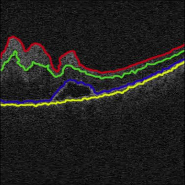
as segmenting the image shown in Figure 2.
Figure 1: Representing a social network as a graph.
Many of these new applications typically model entities Figure 2: Segmentation of medical scans [21].
∗This work is partially supported by NSF grant number
CCF-1018463. I. Koutis is supported by NSF CAREER More intricate uses of electrical networks have been dis-
award CCF-1149048. Part of this work was done while covered in the context of classical graph optimization prob-
I.Koutis was at CMU. R. Peng is supported by a Microsoft lems, with the recent network flow algorithm by Christiano
Research Fellowship. et al. [5] standing out as an algorithmic breakthrough. The
Permission to make digital or hard copies of all or part of this work for algorithms reduce the problem to not just one network, but
personal or classroom use is granted without fee provided that copies are to a sequence of networks via successive readjustment of
not made or distributed for profit or commercial advantage and that copies edges. In these algorithms, some of the resulting systems
bear this notice and the full citation on the first page. To copy otherwise, to are significantly harder than ‘typical’ instances, capturing
republish, to post on servers or to redistribute to lists, requires prior specific –in some sense– the hardness of the optimization problems
permission and/or a fee.
Copyright 2008 ACM 0001-0782/08/0X00 ...$5.00.
themselves.Current SDD solvers are empirically fast for some engi- To compute the upper estimate for the effective resistance
neering applications, but they are not able to efficiently solve of an edge in the modified graph we only use the edges of
most cases of SDD linear systems. Besides these practical the LSST. A key side-effect of this modification is that the
limitations, the fact that existing SDD solvers lack guaran- number of non-tree edges in the preconditioner is much less
tees on arbitrary instances limits their implications to the than the number of edges in the original graph. In this way
theory of algorithms as well. we meet the known design conditions and obtain the faster
These factors underline the need for ‘mathematically certi- solver.
fied’ solvers that are provably fast for arbitrary SDD linear
systems, independently of their origin, be it –for instance–
social or protein networks. This paper describes our state
2. NETWORKS, SYSTEMS, SOLVERS
of the art solver for Symmetric Diagonally Dominant (SDD) Let us consider the problem of finding a voltage setting
linear systems. given the desired net current flow at each of the vertices. A
simple 3-node example of an electric network is depicted in
Figure 3. The inverse of the resistance of wire, also known
1.1 A glimpse at the solver as conductance, is a direct analogue to the edge weight in
The class of SDD linear systems arises in particular in a graph; because of that we choose to label each wire by its
the study of electrical networks, which provide us with a conductance rather than its resistance. Setting the voltages
concept crucial to understanding how our algorithm works: of the vertices to some values leads to an electrical flow
the effective resistance between two points in a network. through the edges. There are two fundamental principles
In addition, the connection to networks enables adopting a governing this voltage setting. (a) Kirchhoff’s law, which
second alternative view of our linear system, as a weighted states that with the exception of the vertices where current
graph. We give the details in Section 2. is injected/extracted, the net flow at each vertex is zero.
We then move to the algebraic component of our solver. (b) Ohm’s law, which states that the current on an edge
The approximate solution of linear systems via iterative meth- equals the voltage difference between its endpoints times
ods is a topic not commonly encountered in computer science the conductance of the wire.
but thoroughly studied in the context of numerical linear As an example consider the network given in Figure 3
algebra and scientific computation. Section 3 explains iter- where we set the voltages at the three vertices to be x1 , x2
ative methods via an analogy with the computation of the and x3 respectively. By Ohm’s law we get that the current
inverse of a real number in a calculator with a broken divi- flows along edges 1 → 2 and 1 → 3 are 1 · (x1 − x2 ) and
sion key, where only addition and multiplication operations 2 · (x1 − x3 ) respectively. Therefore the amount of current
are available. This leads us to preconditioning, a term first we will need to inject into vertex 1 to maintain these voltages
used by Alan Turing. In the graph theoretic context, precon- is:
ditioning provides a measure of similarity between graphs.
This measure is used to formalize design conditions suffi- 1 · (x1 − x2 ) + 2 · (x1 − x3 ) = 3x1 − x2 − 2x3
cient for the construction of a fast iterative method.
Identities for the required current entering/leaving vertices
What distinguishes our solver from classical iterative meth-
2 and 3 can also be derived similarly. Therefore, if we want
ods is its combinatorial component and specifically the
one unit of current to enter at vertex 1 and leave at vertex
use of graph theoretic algorithms. It was understood before
3, the voltages will need to satisfy the following system of
our work that the key to a fast solver is finding a subgraph
linear equations:
(the preconditioner) which is similar to a given graph, but
has substantially fewer edges [20]. Our contribution is a con-
ceptually simple procedure for constructing good precondi-
tioners, this is the topic of Section 4.
The base of our preconditioner is a spanning tree of the in-
put graph, in other words a minimally connected subgraph.
Our algorithm needs a special type of spanning tree called
a low-stretch tree (LSST) which we describe in Section 4.1.
This can be found using very sophisticated but fast algo- Figure 3: A simple network and linear system.
rithms.
To get a better preconditioner we perform random sam- Using more compact notation, linear systems assume the
pling: each edge of the input graph is put into the pre- form Ax = b where x is a n × 1 column vector of unknowns,
conditioner with a specified probability. It was known that also called variables, b is a n × 1 column vector of real num-
the effective resistance between the two endpoints of each bers, and A is an n × n matrix containing the coefficients of
edge provides a good sampling probability for it [18]. Un- the variables. For example, the above linear system can be
fortunately the problem of computing the effective resistance expressed in matrix form as:
seems to require solving an SDD linear system, which is the
3 −1 −2
x1
1
problem we are trying to solve in the first place. −1 2 −1 x2 = 0 . (2.1)
Our main contributions are two ideas that allow us to −2 −1 3 x3 −1
circumvent this ‘chicken and egg’ problem. The first idea
is to use an upper estimate on the effective resistance for Note that each off-diagonal entry is the negation of the
each edge. The second idea is to compute these estimates conductance of the resistor connecting its two vertices, and
on a modified graph, in which the estimates are sufficiently each diagonal entry is the sum of the conductances of all re-
good. The modification is in fact quite simple; we find an sistors incident to the corresponding vertex. Since resistive
LSST of the graph and increase the weight all of its edges. networks can also be viewed as undirected graphs, this typeof matrix is known as a Graph Laplacian and we will rely the breakthrough achievement of Spielman and Teng [19]:
on this connection extensively in our algorithm. Symmet- the first solver that runs in time O(m logc n) for any graph
ric Diagonally Dominant (SDD) matrices are a further Laplacian, where c is a large constant. The work discussed
generalization of graph Laplacians. However, an SDD sys- here, summarized in the following claim from [10], provides
tem can be easily transformed into a Laplacian system (e.g. a conceptually simpler, faster and more practical algorithm.
see [9]) and so we will restrict our attention entirely to graph Theorem. Symmetric diagonally dominant systems can
Laplacians. be solved in Õ(m log n log(1/)) time2 , where is a stan-
Once we’re able to obtain the voltages at each vertex, dard measure of the approximation error.
we can also compute the effective resistance between two
vertices. Intuitively, this notion can be viewed as thinking
of the entire network as a single electrical component. Then 3. THE ALGEBRAIC COMPONENT
by Ohm’s law the voltage drop required to send 1 unit of
current corresponds to the resistance of the component. In 3.1 Iterative methods: Division-free inversion
our example, the effective resistance between vertex 1 and Our way towards the faster solver starts with a basic and
2 is x1 − x3 = 2/5. Formally, this value equals vs − vt from perhaps seemingly unrelated question: is it possible to com-
the solution of the linear system Lv = φ, where φ is zero pute the inverse 1/α of a number α using a calculator with
everywhere except in the two entries corresponding to the a broken division key?
nodes s and t, for which we set φs = 1 and φt = −1. As To answer the question we can invoke a basic identity
we will see later, this metric is not only used for network that tells us that when 0 < α < 2, 1/α equals the following
analytics, but also plays a crucial role in our solver itself. infinite sum:
2.1 Solvers and their speed
1/α = 1/(1 − (1 − α))
Despite its long history, the problem of constructing good
solvers is considered far from being solved, especially in = 1 + (1 − α) + (1 − α)2 + (1 − α)3 + . . . (3.2)
terms of speed. The speed of algorithms is commonly mea-
Of course, computing an infinite sum is not possible. But
sured in terms of the input size. In the case of general linear
keeping a number of terms will give us an approximation of
systems on n variables, the matrix has size n2 . However, ma-
1/α; the more terms we keep the better the approximation.
trices are often sparse, i.e. most of their entries are equal
But how is this related to the problem of solving linear
to zero. Because of this we can easily ‘compress’ them to
systems? Matrices borrow several of the usual properties of
size proportional to the number of non-zeros, denoted by
scalar numbers. When A is symmetric, its inverse A−1 also
m. The best case scenario, which remains entirely consistent
satisfies the identity in 3.2, substituting A for α, A−1 for
with our current understanding, is that linear systems can
1/α and the identity matrix I for the number 1. Further-
be solved with O(m) 1 operations.
more, if we want an approximation to x = A−1 b 3 we can
It’s fair to say that Gaussian elimination is the most well-
actually avoid entirely taking powers of the matrix; the ith
known method for solving linear systems. It runs in O(n3 )
approximate vector
time and it is known as a direct method in that, if the arith-
metic operations are performed exactly then one gets the x(i) = (I + (I − A) + . . . (I − A)i )b
exact solution to the system. Although this exponent of 3
has been decreased to as low as 2.37 [24], direct methods in can be produced with i applications of the following simple
general require storing n2 entries, creating a natural bottle- recurrence:
neck that limits us to systems with a few thousand variables.
x(0) =0
One possible remedy to the space and time limitations
of direct methods are iterative methods. These compute x(i+1) =b + (I − A)x(i) for i > 0.
progressively better approximate solutions by only perform-
ing matrix-vector products and other simpler vector op- It can be seen that each step involves a matrix-vector mul-
erations. tiplication by A. This is the simplest among iterative meth-
One of the most important iterative methods is Conjugate ods that in general attempt to approximate the solution of
Gradient, discovered by Lanczos, Hestenes and Stiefel in the a linear system using only a sum of results from a series of
early 1950s. This method works for arbitrary symmetric matrix-vector multiplications.
positive definite systems, a class that includes SDD systems.
While it requires only O(m) space, it is understood that its
3.2 Preconditioning
running time –in its original form– can be large. So far, our replacement for the division button is of rather
Strong evidence that iterative methods can combine low restricted value, since it only works when 0 < α < 2, and
space requirements and very fast running time was provided can converge very slowly when α is close to 0 or 2. One
by a family of iterative methods known as multigrid [22]. way to extend our method and to speed up its convergence
Multigrid solvers have an O(m) running time guarantee al- is to add a ‘restricted division’ key to our calculator. This
beit for restricted and well-structured systems that arise in key allows us to ‘divide’ by a fixed scalar β of our choice,
scientific computing. which in the matrix setting corresponds to a matrix-vector
The solver we will review in this paper is also an iterative product involving the inverse, B −1 of a matrix B. We can
method. It is the culmination of a line of work initiated speed up our algorithm by pressing the ‘restricted division’
by Vaidya [23], which was brought to near-completion with 2
The Õ() notation hides a log log n factor.
1
We use f (n) = O(g(n)) to denote f (n) ≤ c · g(n) when
3
If A−1 doesn’t exist, as in the case of Laplacians, we use
n ≥ n0 for some constants c and n0 . A−1 to denote the pseudoinverse as well.button after each matrix-vector multiplication by A, giv-
ing the following modified recurrence known as precondi-
tioned Richardson iteration:
x(0) =0
x(i+1) =B −1 b + (I − B −1 A)x(i) for i > 0.
The matrix B is known as the preconditioner and in-
stead of solving the system Ax = b, we are essentially solv-
ing the preconditioned system: B −1 Ax = B −1 b. It is
worth emphasizing that each step of this method involves
a matrix-vector multiplication by A followed by a ‘division’ Figure 4: Two similar graphs: A complete graph and
by the matrix B. a random small subset of its edges, made heavier.
3.3 Measuring similarity between matrices
Looking back at the single variable recurrence, the critical To evaluate B −1 y we do not need to compute B −1 . We
condition for its convergence is 0 < α < 2. An extension can instead solve the system Bz = y; the solution z will be
of it is needed in order to analyze preconditioned iterative equal to B −1 y. Clearly, we would like to solve systems in-
methods involving matrices A and B. For matrices A and volving B as quickly as possible. At the same time we would
B, we say A B when for all vectors x we have like the number of iterations to be as small as possible, since
each of them requires at least m operations. Furthermore,
xT Bx ≤ xT Ax. a slow algorithm for computing the preconditioner B would
defeat the purpose of a fast solver. So, we should also be
Unlike the situation with scalars, this ordering is only ‘par- able to find B quickly. Balancing these three opposing goals
tial’. Even for size 2 diagonal matrices, it is possible that makes the problem quite challenging.
neither B A nor A B holds. But when A and B are
symmetric, there will be numbers κmax and κmin such that:
3.6 Recursion and design conditions
In order to solve the linear system fast, we will need a pre-
κmin A B κmax A. conditioner B which is an extremely good approximation
We will say that B is a κ-approximation of A, where of A and can be solved in linear time. Satisfying both these
κ = κmax /κmin . In this case, after introducing additional requirements is too much to hope for. In practice any good
scaling factors, it can be shown that the preconditioned graph preconditioner B won’t be significantly easier to solve
Richardson’s iteration gives a good approximation in O(κ) comparing to A. As a result, there is no hope that precon-
iterations. There are iterative methods with faster conver- ditioned Richardson’s iteration or any other preconditioned
gence rates, and –as we will see- our solver relies on one of method can lead to fast solvers.
them, known as Chebyshev iteration. The remedy to the problem is recursion. In a recursive
preconditioned method, the system in the preconditioner B
3.4 Interpreting similarity is not solved exactly but approximately, via a recursive in-
It is interesting to see what this measure of similarity vocation of the same iterative method. We now have to find
means in the context of electrical networks, that is when a preconditioner for B, and furthermore a preconditioner
both A and B are Laplacians. The quadratic form for it and etc. This produces a multilevel hierarchy of
progressively smaller graphs.
xT Ax
is equal to the energy dissipation of the network A, when
the voltages at vertices are set to the values in the vector x.
Then, the network B is a κ-approximation of the network A
whenever for all voltage settings, B dissipates energy which
is within a κ factor of that dissipated by A.
So, roughly speaking, two networks are similar when
their ‘energy profiles’ are similar. This definition doesn’t
necessarily correspond to intuitive notions of similarity; two
networks may appear to be very different but still be similar.
An example is shown in Figure 4.
3.5 What is a good preconditioner?
Figure 5: The sequence of calls of a recursive itera-
Armed with the measure of similarity, we’re now ready tive method. The matrix is fixed at each level.
to face the central problem in solver design: how do we
compute a good preconditioner? Rohklin, Spielman and Teng [19] analyzed a recursive it-
To deal with the question we must first understand what erative method which moves between levels of the hierarchy
properties are desirable in a preconditioner. A big unknown as shown in Figure 5; for each visit at level i, the algorithm
in the total running time is the cost incurred by the limited makes k visits to level i+1. Every time the algorithm returns
division button that evaluates B −1 y. to the ith level it performs matrix-vector multiplicationswith the graph Ai , and other simpler operations; so the work weighted graphs, where all trees have equal weight.
is proportional to the number of edges of Ai . To keep the The key to finding a good tree to use as a building base
total work as small as possible, i.e. O(km), the graphs in is the notion of stretch: For every edge (u, v) of the graph,
the hierarchy must get smaller sufficiently fast. In partic- there is a unique ‘detour’ path between u and v in a tree
ular, it is sufficient that the graph on level i + 1 is smaller T . The stretch of the edge with respect to T is equal to
than the graph on level i by a factor of 1/(2k). the distortion caused by this detour, and in the unweighted
However, the algorithm must converge within the O(km) case, it’s simply the length of the tree path. This notion
time bound. To achieve this the iterative method analyzed generalizes naturally to the weighted case, which we’ll for-
within this recursive framework is a method known as Cheby- malize in Section 4.3. The total stretch of a graph A with
shev iteration. It requires only O(k) iterations, when B is respect to a tree T is the sum of the stretches of all the
a k2 -approximation of A, as compared to the O(k2 ) iter- off-tree edges. A low-stretch tree (LSST) is one for which
ations required by Richardson’s iteration. Using this fact we have a good upper bound on the total stretch. So, at a
Spielman and Teng arrived at design conditions that are high level, an LSST has the property that it provides good
sufficient for a fast solver [20]. It was actually shown that (on average) ‘detours’ for edges of the graph. A concrete
a good algorithm for preconditioning extends to a good example on a larger unweighted graph is given in Figure 6,
solver. More specifically, assume that for some fixed value where the tree on the right has lower total stretch, and as it
C and any value of k, we have a fast algorithm that given A, turns out is a better base tree to add edges to.
produces a k2 -approximation with n + C · m/k edges. Then
we automatically get a solver that runs in time O(k · m).
Carefully checking the above statement, we realize that
there is a slight discrepancy. If m is close to n and k is
large, then n + C · m/k will be bigger than m, which contra-
dicts our promise for a multilevel hierarchy of progressively
smaller graphs. However, as observed by Vaidya [23], when
m is almost the same n, the graph has several ‘tree-like’
parts, and these can be reduced via a ‘partial’ Gaussian
elimination that runs in O(m) time. So whenever this case
appears, it makes sense to first run partial elimination. This Figure 6: Two possible spanning trees of the un-
will decrease the vertex count n, leading to a much smaller weighted square grid, shown with red edges.
instance on which recursion is applicable.
The multilevel analysis of Spielman and Teng is significant
not only for its actual algorithmic value but also the concep- Trees for the grid: a quantitative example
tual reduction of the multi-level solver design problem to a The two spanning trees of the 8 × 8 grid shown
√ in √
Figure 6
well-defined two-level preconditioning problem, allowing us can guide our understanding of the general n × n grid.
now to focus on the combinatorial component of the solver.
In the√tree on the left,
√ for each vertical edge beyond col-
umn n/2, at least n horizontal edges are needed to
4. THE COMBINATORIAL COMPONENT travel between
√ its endpoints; that means that its stretch
Although graph theory has been used to speed up direct is at least n. So the n/2 edges in the right half of the
square grid contribute a total stretch of n1.5 .
methods, it took a paradigm-shifting idea of Pravin Vaidya
to enter a systematic study of using graph theory for it- In the tree on the right, all edges
√ along the middle row and
erative methods. In particular, Vaidya suggested the use of column still have stretch O(
√ n). However, the middle row
a spanning tree of the graph A as a building base for and column only have O( n) edges and so they contribute
only O(n) to the total stretch. Recall that all we need is a
the preconditioner B. A spanning tree of a graph is a con- low total stretch, so a small number of high-stretch edges
nected subgraph without loops. The choice of a tree stems is permitted. Having accounted for the edges in the middle
from the observation that linear systems whose matrix is the row and column, the argument can then be repeated on
Laplacian of a tree can be solved in O(n) time via Gaussian the 4 smaller subgraphs of size n/4 formed by removing
elimination. Adding a few edges of A back onto the tree the middle row and column. These pieces have trees that
returns a preconditioner B which can only be better than are constructed similarly, leading to the recurrence
the tree, while still being relatively easy to solve. Vaidya’s TotalStretch(n) = 4 ∗ TotalStretch(n/4) + O(n).
idea set forth two questions: (i) What is an appropriate
base tree? (ii) Which off-tree edges should be added into Its solution is TotalStretch(n) = O(n log n).
the preconditioner? A generalization of this type of ‘accounting’, that keeps
While these questions seem to be interrelated, we can ac- the number of high stretch edges small, forms the basis of
tually address them separately. the current state-of-the-art algorithms [1].
4.1 Low-stretch: The base spanning tree
The goal of finding a preconditioning tree B which is as Algorithms for the computation of LSSTs were first stud-
similar as possible to the graph A led Vaidya to a natural ied in an unrelated context [2], where it was shown that any
idea: use a tree which concentrates the maximum possible graph contains a spanning tree with total stretch O(m1+ );
weight from the total weight of the edges in A. the tree can be found in O(m log n) time. The total stretch
The maximum-weight spanning tree idea led to the first was lowered to O(m log2 n) in [6], and further to Õ(m log n)
non-trivial results, but does not suffice for our algorithm. in [1], giving the following theorem.
In fact, the weight measure doesn’t distinguish trees in un- Theorem. Every graph has a spanning tree of totalstretch Õ(m log n). The tree can be found in Õ(m log n)
Understanding re-weighting
time.
While it may appear complicated, the re-weighting choice
Boman and Hendrickson first introduced LSSTs as stand
is quite natural. The reasoning is that the ‘expected value’
alone preconditioners in 2001. This was a catalyst to sub-
of B should be A itself on an edge-to-edge basis. In other
sequent progress, which used LSSTs as a base for building
words, the average of many B’s output by the algorithm
even more intricate preconditioners. In fact, LSSTs are in-
should be A itself.
dispensable components of all nearly-linear time SDD sys-
tem solvers. It is worth pointing out that while LSSTs were Spielman and Srivastava found the probabilities that give
originally conceived as potentially good two-level precondi- sparsifiers with the fewest number of edges with the help of
tioners, their full power in the context of multilevel solvers some experimentation. Amazingly, the answer turned out
wasn’t realized until our work, which we describe in Sec- to be related to the effective resistance of the edge, specifi-
tion 4.3. cally te = we Re . With hindsight, it is interesting to reflect
about the natural meaning of effective resistance. If there is
a wire of resistance re = 1/we , between i and j, the effec-
tive resistance Re will in general be smaller than re because
most probably there will be other network connections to
accommodate the flow; this is known as Rayleigh’s mono-
tonicity theorem. The extreme case we Re = 1 occurs only
when there is no other route between i and j except the wire
4.2 Sparsification joining them. In this situation, the edge (i, j) is crucial for
the network. On the other hand if we Re is very small, there
Spielman and Teng’s [19] main contribution was a ‘tour de
must be significant alternative network connections between
force’ algorithm for finding a preconditioner that’s the LSST
(i, j). Therefore, the product we Re as a measure of the im-
plus a small number of edges. It took many by surprise as
portance of a wire. Using tools from modern matrix theory
it yielded the first nearly-linear time SDD solver.
[15], Spielman and Srivastava proved that this algorithm
Describing the algorithm is out of the scope of this article,
does return a good spectral sparsifier
P with high probability.
but it is worth noting its two enhancements over previous
Combining with the fact that t = e we Re = n − 1 yields
approaches. First, instead of just adding off-tree edges from
the overall number of edges: O(n log n).
A back onto the tree, the algorithm re-weights them. The
Despite being a major improvement in the theory of graph
tree edges may themselves be re-weighted in the final pre-
sparsification, the algorithm of Spielman and Srivastava did
conditioner B. Second, the procedure for adding edges in
not accelerate the SDD solver as current methods for quickly
B is not deterministic but randomized, as it contains a
computing effective resistances require the solution of linear
process for sampling edges from A.
systems. The guarantee of O(n log n) edges is also hard to
However the major conceptual and technical contribu-
connect with the n + C · m/k edges needed by the design
tion of Spielman and Teng that formed the cornerstone of
condition. However, it is fair to say that their result cleared
their solver was a sparsification algorithm. They showed
the way to our contribution to the problem.
that every graph A has a 2-approximation B which has
O(n logc n) edges for some large constant c. The graph B
is called the sparsifier and, of course, it can be used as a 4.3 Which off-tree edges?
preconditioner when A is dense. If we can’t effectively compute effective resistances, can
After the first sparsification result, progress towards faster we at least approximate them quickly, even poorly? A closer
SDD solvers took a detour through the study of spectral look at the matrix concentration bounds allows us to relax
sparsification as a stand-alone problem. Works by Batson, this goal a bit further: the sampling algorithm described in
Kolla, Makarychev, Saberi, Spielman, Srivastava and Teng Section 4.2 can be shown to work with any choice of te , as
led to nearly-optimal spectral sparsifiers, albeit at the cost long as te ≥ we Re . The observant reader may notice that
of much higher running time. These results were motivated the expected number of times e is picked is O(te log n), so
by the work of Spielman and Srivastava [18], who gave an increasing te only results in more copies of e being picked
extremely simple algorithm for finding spectral sparsifiers without affecting the expectations of all other edges.
with only O(n log n) edges. Their algorithm, as well as the The intuition that the low-stretch spanning tree must be
Spielman-Teng spectral sparsification algorithm builds upon part of the preconditioner leads us to taking tree-based esti-
a framework established by Benczur and Karger for sampling mates Re0 for the effective resistances Re . In particular, for
and re-weighting a graph. an off-tree edge e we let Re0 be the sum of the resistances
The framework requires positive numbers te assigned to along the unique path between the endpoints of e in the tree,
each edge, corresponding to the relative probabilities of sam- as shown in Figure 7. By Rayleigh’s monotonicity theorem,
pling them. It calculates the sum of these numbers, t =
P we know that this estimate will be higher than the actual
e te and proceeds for O(t log n) rounds. In each round one Re . This leads to the tree-based sampling probability for an
new edge is added to the sparsifier B. The edge is picked off-tree edge e being proportional to te = we Re0 . Further-
randomly with replacement among the m edges of A, but more, if we keep the entire tree in B, we can modify the
not in a ‘fair’ way. An edge e is picked with relative proba- sampling algorithm presented in Section 4.2 to only sample
bility te , which equates to a probability of pe = te /t. Once off tree edges. Then the total number of off-tree (multi)
an edge is picked, it is added to B with weight scaled down edges sampled in B is O(t log n) where t is the sum of all
by a factor of O(te log n). Furthermore, if an edge is picked te s, which in turn . This brings us to the question: how big
twice or more during this process, each new copy is added is t?
as a parallel edge, making B potentially a multi-graph. This question leads us back to the discussion of low-stretchchy, until what is left is the tree itself. This justifies thinking
2 of a low-stretch spanning tree as a graph spine, and is de-
5 picted in Figure 8.
4
2
Figure 7: The effective resistance Re0 of the blue off-
tree edge in the red tree is 1/4 + 1/5 + 1/2 = 0.95. Its
stretch we Re0 is (1/4 + 1/5 + 1/2)/(1/2) = 1.9
spanning tree and the definition of stretch for the gen-
eral weighted case: if we view the length of an edge e as
the inverse of its weight, then its stretch equals to we Re0 4 .
Therefore, t is the total stretch of the off-tree edges with
respect to the tree. Then, using the low-stretch spanning Figure 8: Low-stretch spanning tree as a spine.
tree of the Theorem in Section 4.1, we can upper bound t The ‘cloud’ of off-tree edges becomes progressively
by O(m log n). Recall that the number of samples will be sparser.
t log n and so it appears that we don’t gain much from the
sampling process unless the graph A has a very special tree. When the sparsifier B is viewed as a graph, it’s possible
Our key idea is to make a special graph à out of A. We do for some of its edges to have high stretch. However, a more
so by scaling up, by a factor of κ, the weights of edges of a careful reexamination of the sampling algorithm shows that
low-stretch spanning tree in A. For an edge that’s not part these edges are the result of an edge being sampled many
of the tree, its weight does not change, while the tree path times. From this perspective, these heavy edges are in fact
connecting its endpoints is now heavier by a factor of κ. So many multi-edges, each with low stretch. Therefore, if we
the stretch decreases by a factor of κ and the total stretch of process these multi-edges separately, the tree TA will be a
these edges becomes t = O(m log n/κ). Now, consider what low-stretch spanning tree in B, and the higher edge count
is still bounded by the number of rounds made by the sam-
happens if we sample the off-tree edges in Ã. The output
pling algorithm. This allows us to use TA as a low-stretch
B will be a 2-approximation of Ã. On the other hand, the
spanning tree and sample the off-tree edges in B according
graph à is a κ-approximation to A, and by transitivity B is
to it. Note that with this modification, it’s possible for us
2κ-approximation to A. Also, the number of non-tree edges
to observe a temporary ‘slow down’ in the reduction of the
sampled will be O(t log n) = O(m log2 n/κ). Adding in the
overall edge count; the preconditioner of B may have the
n−1 tree edges gives a total of n+O(m log2 n/κ) edges in B.
same number of off-tree edges as B itself. However the to-
Recall that the two-level design conditions stated in Sec-
tal number of multi-edges will decrease at a rate that meets
tion 3.6 require a k2 -approximation with n + C · m/k edges
the design conditions. This reuse of the tree for generating
in order to obtain a running time of O(k·m). So by setting κ
sparsifiers is a crucial deviation from prior works.
to O(log4 n), we meet the conditions with k = O(log2 n) and
But this doesn’t fully explain the faster solver algorithm.
arrive at our first result:
To achieve it we need an extra trick. Assume for a moment
Theorem [9]. Symmetric diagonally dominant systems that our graph A is what we call spine-heavy; that is,
can be solved in Õ(m log2 n log(1/)) time, where is a it has a tree of total stretch equal to O(m/ log n). Then
standard measure of the approximation error. by an argument analogous to the one using a standard low
As it turned out, the low-stretch spanning tree is not only a stretch spanning tree, we can show that B actually satisfies
good base tree, but also tells us which off-tree edges should the two-level preconditioning requirement for an even lower
go to the preconditioner. Our faster, O(m log n) time al- value of κ, namely a fixed constant. This, in combination
gorithm will come via an even better understanding of the with spine-based sampling allows us to solve spine-heavy
properties of the tree. graphs in linear time. A more global view of this algorithm,
as shown in Figure 8 is that it progressively makes the tree
4.4 The final push: Low-stretch spine heavier, while removing off-tree ones.
Assume that we’re given a graph A, found its low-stretch Since our initial graph A can’t be expected to be spine-
tree TA , and based on it, computed the preconditioner B. heavy, we make a spine-heavy graph à out of A, by scaling-
Then the O(m log2 n) time solver algorithm dictates that we up its low-stretch tree by an O(log2 n) factor. Now à is
recursively do the same with B. But do we really have to an O(log2 n)-approximation to A and we can solve it in
scrap TA and find another low-stretch tree TB ? After all, it O(m) time. Using it as preconditioner for A completes the
may be the case that TA is a low-stretch tree of B, or close O(m log n) time solver. So, we have arrived at our destina-
to being one. tion.
What the O(m log2 n) algorithm [9] missed is the obser- Theorem [10]. Symmetric diagonally dominant systems
vation that we can keep sampling based on the same can be solved in Õ(m log n log(1/)) time, where is a
tree, gradually generating all levels of the multilevel hierar- standard measure of the approximation error.
4
An alternate view is that the stretch of e is the weighted
length of the tree path between e’s end points divided by e’s
own length. 5. EXTENSIONS5.1 Parallelization number of edge disjoint routes (or ‘flow’) between two nodes
Several algorithms in numerical linear algebra have par- s and t. Further work in this direction led to the first im-
allel versions that are work-efficient. A parallel algorithm is provement in 20 years on the approximate maximum flow
called work-efficient if it performs roughly the same work problem [5]. The max-flow result is in turn directly applica-
as its best sequential algorithm for the same problem, while ble to graph partitioning, i.e. the separation of a graph to
allowing the use of parallel processing. two well connected pieces; the fastest known algorithm for
The first steps towards studying the parallelism poten- this problem repeatedly applies the fast max-flow algorithm
tial of SDD solvers were taken in [3], which presented a [16].
nearly (up to log factors) work-efficient algorithm, running It is also worth noting that the solver presented in [3]
in O(m1/3 ) parallel time. Informally, this means that up to readily gives –for all the above problems- parallel algorithms
that are essentially able to split evenly the computational
m2/3 parallel processes can be used to accelerate the algo-
work and yield speedups even when only a small number of
rithm, a non-trivial potential for parallelism.
processors is available. This is a rare feature among previous
5.2 Implementation algorithms for these problems.
Solver-based algorithms have already entered practice, par-
The most complicated component of our solver is the al- ticularly in the area of computer vision, where graphs are
gorithm for computing a low-stretch tree. It is however ex- used to encode the neighboring relation between pixels. Sev-
pected that a conceptually simpler algorithm for this prob- eral tasks in image processing, such as image denoising,
lem is to be discovered, leading to a fast and ‘clean’ im- gradient inpainting, or colorization of grayscale images, are
plementation, and quite likely the removal of the log log n posed as optimization problems for which the best known
factors from the running time. algorithms solve SDD systems [11, 12]. Linear systems in
In a practical implementation, it would be a good idea to vision are often ‘planar’, a class of SDD systems for which
substitute the recursive preconditioned Chebyshev iteration an O(m) time algorithm is known [7].
by a recursive preconditioned Conjugate Gradient (PCG) Given the prevalence of massive graphs in modern prob-
iteration. It is known that, in two-level methods, PCG is lems, it is expected that the list of applications, both theo-
essentially able to automatically optimize the performance retical and practical, will continue expanding in the future.
of the preconditioner. It is expected that the same should We believe that our solver will accelerate research in this
be true for some multilevel variant of PCG, but this is yet area and will move many of these algorithms into the prac-
to be proven. tical realm.
We expect that, eventually, the best implementations of
SDD solvers will combine ideas from this work and other
existing graph-based techniques [8], or entirely new ideas. 7. REFERENCES
Such ideas will certainly be needed to achieve –if possible– [1] I. Abraham and O. Neiman. Using petal
a ‘fully parallel’, O(log n) time, work-efficient SDD solver. decompositions to build a low stretch spanning tree.
In Proceedings of the 44th symposium on Theory of
Computing, STOC ’12, pages 395–406, New York, NY,
6. THE LAPLACIAN PARADIGM USA, 2012. ACM.
Solvers for SDD systems are increasingly viewed as an [2] N. Alon, R. Karp, D. Peleg, and D. West. A
algorithmic primitive; a fundamental subroutine that can graph-theoretic game and its application to the
be used to design many other efficient algorithms. Indeed, k-server problem. SIAM J. Comput., 24(1):78–100,
since the Spielman-Teng breakthrough, the availability of 1995.
fast SDD solvers has sparked what has been dubbed the
[3] G. E. Blelloch, A. Gupta, I. Koutis, G. L. Miller,
Laplacian paradigm: an entire class of new algorithms
R. Peng, and K. Tangwongsan. Near linear-work
spanning various areas. Because it is impossible to do justice
parallel SDD solvers, low-diameter decomposition, and
to each one of these topics, we will present some unifying
low-stretch subgraphs. In Proceedings of the 23rd
themes and only point to some representative examples of
ACM symposium on Parallelism in algorithms and
applications.
architectures, SPAA ’11, pages 13–22, New York, NY,
Perhaps the most direct example of using the solver as a
USA, 2011. ACM.
primitive is the computation of eigenvectors. It was shown
in [20] that O(log n) iterations of solves produce a good ap- [4] E. G. Boman, B. Hendrickson, and S. A. Vavasis.
proximation to a basic eigenvector of a graph. More closely Solving elliptic finite element systems in near-linear
related to preconditioned iterative methods is a solver for time with support preconditioners. SIAM J.
elliptic finite element linear systems [4]. This work showed Numerical Analysis, 46(6):3264–3284, 2008.
that such systems can be preconditioned with graph Lapla- [5] P. Christiano, J. A. Kelner, A. Ma̧dry, D. Spielman,
cians and so they can be solved in nearly-linear time. and S.-H. Teng. Electrical Flows, Laplacian Systems,
A more general framework stems from one of the most and Faster Approximation of Maximum Flow in
powerful discoveries in combinatorial optimization: interior Undirected Graphs. In Proceedings of the 43rd ACM
point algorithms. It was shown by Daitch and Spielman [17] Symposium on Theory of Computing (STOC), 2011.
that interior point algorithms allow us to reduce a broad [6] M. Elkin, Y. Emek, D. A. Spielman, and S.-H. Teng.
class of graph problems to solving a small number of SDD Lower-stretch spanning trees. In Proceedings of the
linear systems. This led to the best known running times 37th Annual ACM Symposium on Theory of
for problems such as minimum cost flow and loss generalized Computing (STOC), pages 494–503, 2005.
flow. These problems are extensions of the maximum flow [7] I. Koutis and G. L. Miller. A linear work, O(n1/6 )
problem, which in its simplest version asks for the maximum time, parallel algorithm for solving planar Laplacians.In Proc. 18th ACM-SIAM Symposium on Discrete [22] U. Trottenberg, A. Schuller, and C. Oosterlee.
Algorithms (SODA), 2007. Multigrid. Academic Press, 1st edition, 2000.
[8] I. Koutis and G. L. Miller. Graph partitioning into [23] P. M. Vaidya. Solving linear equations with symmetric
isolated, high conductance clusters: Theory, diagonally dominant matrices by constructing good
computation and applications to preconditioning. In preconditioners. A talk based on this manuscript was
Symposiun on Parallel Algorithms and Architectures presented at the IMA Workshop on Graph Theory and
(SPAA), 2008. Sparse Matrix Computation, October 1991.
[9] I. Koutis, G. L. Miller, and R. Peng. Approaching [24] V. Vassilevska Williams. Breaking the
optimality for solving SDD systems. In Proceedings of Coppersmith-Winograd barrier. In Proceedings of the
the 51st Annual IEEE Symposium on Foundations of 44th symposium on Theory of Computing, STOC ’12,
Computer Science, FOCS. IEEE Computer Society, 2012.
2010.
[10] I. Koutis, G. L. Miller, and R. Peng. A near-m log n
solver for SDD linear systems. In Proceedings of the
52nd Annual IEEE Symposium on Foundations of
Computer Science, FOCS. IEEE Computer Society,
2011.
[11] I. Koutis, G. L. Miller, and D. Tolliver. Combinatorial
preconditioners and multilevel solvers for problems in
computer vision and image processing. Computer
Vision and Image Understanding, 115(12):1638–1646,
2011.
[12] D. Krishnan and R. Szeliski. Multigrid and multilevel
preconditioners for computational photography. ACM
Trans. Graph., 30(6):177, 2011.
[13] D. Liben-Nowell and J. M. Kleinberg. The
link-prediction problem for social networks. JASIST,
58(7):1019–1031, 2007.
[14] P. V. Missiuro, K. Liu, L. Zou, B. C. Ross, G. Zhao,
J. S. Liu, and H. Ge. Information flow analysis of
interactome networks. PLoS Comput Biol,
5(4):e1000350, 04 2009.
[15] M. Rudelson and R. Vershynin. Sampling from large
matrices: An approach through geometric functional
analysis. J. ACM, 54(4):21, 2007.
[16] J. Sherman. Breaking
√ the multicommodity flow
barrier for O( log n)-approximations to sparsest cut.
In Proceedings of the 2009 50th Annual IEEE
Symposium on Foundations of Computer Science,
FOCS ’09, pages 363–372, Washington, DC, USA,
2009. IEEE Computer Society.
[17] D. A. Spielman and S. I. Daitch. Faster approximate
lossy generalized flow via interior point algorithms. In
Proceedings of the 40th Annual ACM Symposium on
Theory of Computing (STOC), May 2008.
[18] D. A. Spielman and N. Srivastava. Graph
sparsification by effective resistances. In Proceedings of
the 40th Annual ACM Symposium on Theory of
Computing (STOC), pages 563–568, 2008.
[19] D. A. Spielman and S.-H. Teng. Nearly-linear time
algorithms for graph partitioning, graph sparsification,
and solving linear systems. In Proceedings of the 36th
Annual ACM Symposium on Theory of Computing
(STOC), pages 81–90, June 2004.
[20] D. A. Spielman and S.-H. Teng. Nearly-linear time
algorithms for preconditioning and solving symmetric,
diagonally dominant linear systems. CoRR,
abs/cs/0607105, 2006.
[21] D. A. Tolliver, I. Koutis, H. Ishikawa, J. S. Schuman,
and G. L. Miller. Automatic multiple retinal layer
segmentation in spectral domain oct scans via spectral
rounding. In ARVO Annual Meeting, May 2008.You can also read