Real-Time Selfie Video Stabilization - arXiv
←
→
Page content transcription
If your browser does not render page correctly, please read the page content below
Real-Time Selfie Video Stabilization

                                                           Jiyang Yu1,3 Ravi Ramamoorthi1 Keli Cheng2 Michel Sarkis2 Ning Bi2
                                          1
                                              University of California, San Diego 2 Qualcomm Technologies Inc. 3 JD AI Research, Mountain View
                                                             jiy173@eng.ucsd.edu              ravir@cs.ucsd.edu     {kelic,msarkis,nbi}@qti.qualcomm.com
arXiv:2009.02007v2 [cs.CV] 16 Jun 2021

                                         Figure 1. Our method stabilizes selfie videos using A background feature points and foreground face vertices in each frame. B The two-
                                         branch stabilization network infers C the moving least squares (MLS) warping for each frame. D We show the face and background motion
                                         of the input vs. our stabilized result. For visualization only, the background tracks are computed from the translation component of the
                                         homography between consecutive frames. The face tracks are computed from the centroid of the fitted face vertices in each frame.

                                                                           Abstract                               tion algorithms since tracking the frame motion is difficult
                                                                                                                  in the presence of large occlusion. The second step is to
                                             We propose a novel real-time selfie video stabilization              replan/stabilize the motion. In selfie videos, the motions in
                                         method. Our method is completely automatic and runs at                   foreground/background are usually very different. Existing
                                         26 fps. We use a 1D linear convolutional network to di-                  selfie video stabilization methods like [19] aim to stabilize
                                         rectly infer the rigid moving least squares warping which                the face. However, stabilizing according to only foreground
                                         implicitly balances between the global rigidity and local                results in significant shake in the background, and vice versa.
                                         flexibility. Our network structure is specifically designed              The third step is the warping of the frames. For selfie videos,
                                         to stabilize the background and foreground at the same                   the users are sensitive to distortion on the human face. This
                                         time, while providing optional control of stabilization fo-              requires high rigidity in the foreground warping while main-
                                         cus (relative importance of foreground vs. background) to                taining the flexibility in the background warping.
                                         the users. To train our network, we collect a selfie video
                                                                                                                      Critically, consumer applications like selfie video stabi-
                                         dataset with 1005 videos1 , which is significantly larger than
                                                                                                                  lization require a significantly fast or even real-time online
                                         previous selfie video datasets. We also propose a grid ap-
                                                                                                                  algorithm to be practical. This rules out most video stabiliza-
                                         proximation to the rigid moving least squares that enables
                                                                                                                  tion algorithms requiring high overhead pre-processing like
                                         the real-time frame warping. Our method is fully auto-
                                                                                                                  SFM [10], optical flow [15, 25, 4] and future motion informa-
                                         matic and produces visually and quantitatively better results
                                                                                                                  tion [6, 11]. A previous selfie video stabilization method [24]
                                         than previous real-time general video stabilization meth-
                                                                                                                  is an optimization based method and cannot achieve real-
                                         ods. Compared to previous offline selfie video methods,
                                                                                                                  time performance. Although another selfie video stabiliza-
                                         our approach produces comparable quality with a speed
                                                                                                                  tion work Steadiface [19] achieves real-time performance, it
                                         improvement of orders of magnitude. Our code and selfie
                                                                                                                  only estimates global homography for stabilization and can-
                                         video dataset is available at https://github.com/
                                                                                                                  not handle non-linear local motions, e.g. rolling shutter. Ad-
                                         jiy173/selfievideostabilization.
                                                                                                                  ditionally, their work also requires gyroscope information.
                                         1. Introduction                                                              In this paper, we propose a novel learning based real-time
                                             Selfie videos are pervasive in daily communications.                 selfie video stabilization method. Our method is fully auto-
                                         However, capturing high quality selfie video is challenging              matic and requires no preprocessing and user assistance. The
                                         without specialized stabilization devices like gimbals, which            method is designed to tackle the challenges discussed above.
                                         is not convenient, and may not even be allowed in some                   An overview of our method is shown in Fig. 1. To achieve
                                         cases. On the other hand, from the perspective of algorithms,            real-time performance, our method is purely 2D video stabi-
                                         selfie video stabilization is also challenging. In general, there        lization, meaning that our method only depends on the mo-
                                         are three major steps in video stabilization algorithms. The             tion of sparse 2D points detected from input video (Fig. 1 A ).
                                         first step is to detect the motion in the input video. Selfie            This makes our method significantly faster than the offline
                                         videos have a significant foreground occlusion imposed by                selfie video stabilization [24]. In the first step, we avoid the
                                         human, which is a common limitation of video stabiliza-                  occlusion problem by training a segmentation network to in-
                                                                                                                  fer the foreground regions and remove the feature points in
                                              1 The   dataset is collected at UC San Diego.                       the foreground. To take foreground motion into considera-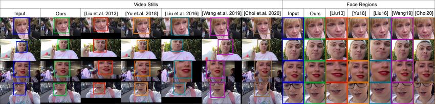
tion, we use the 3DDFA [26] to fit a 3D mesh to video frames.                     with hundreds of warp nodes requires a significant amount of
    To warp the original frames into stabilized frames, we use                    time to warp a frame. We use a sparse grid to approximate
the rigid moving least squares (MLS) [18] (Fig. 1 C ). In                         the MLS warping (Sec. 5) that improves the warping speed
our method, we directly use the background feature points                         by two orders of magnitude. Our entire pipeline is able to
as the warp nodes so that the face shape remains undistorted.                     stabilize the video at 26fps.
Since the original MLS warping is computationally expen-                             3) A novel large selfie video dataset with per-frame la-
sive, we use a grid approximation to maintain the real-time                       beled foreground masks. We will discuss the details of our
performance. Although faster warping methods exist, e.g. as-                      dataset in Sec. 4.1. The dataset enables the training of the
similar-as-possible warping in Liu et al. [14], MLS warping                       foreground detection network and the stabilization network
is necessary for our method. First, traditional grid warping                      in our paper. We will make our dataset publicly available for
requires an additional hyperparameter to regularize the grid                      face and video related researches.
shape. These terms usually conflict with the motion loss and
manually setting the weight between visual distortion and sta-                    2. Previous Work
bility is tricky. On the other hand, MLS warping guarantees
rigidity implicitly and does not require human intervention.                          While video stabilization has been extensively studied,
It also preserves the original shape of regions that lack warp                    most of the works belong to the offline video stabilization
nodes. Second and more importantly, our method is learning                        category. The major reason is that most video stabilization
based instead of optimization based. In the traditional opti-                     methods rely on temporally global motion information to
mization process, it is easy to define the mapping between                        compute the warping for the current frame. Recent works us-
grid vertices and their enclosed feature points in the Jaco-                      ing global motion information include the L1 optimal camera
bian. However, learning this spatial relation between feature                     paths [6], bundled camera paths [14], subspace video stabi-
points and grid vertices is difficult and suffers from general-                   lization [11], video stabilization using epipolar geometry [5],
ization problems. In Sec. 6 and the supplementary video, we                       content-preserving warps [10] and spatially and temporally
will show that our setup with MLS warping directly defined                        optimized video stabilization [22]. These works all involve
on unstructured warp nodes (feature points) is more effective                     the detection of feature tracks and smoothing under certain
than directly learning the grid like Wang et al. [21].                            constraints. Some works use optical flow [15, 25] or video
    The core of our method is the stabilization network                           coding [12] instead of feature tracking as the motion detec-
(Fig. 1 B ). The network generates the displacement of the                        tion method. However, they still inherently require future
warp nodes from the input face vertices and feature points,                       motion information for the global motion optimization.
so that motions of both the foreground (represented by face                           One may argue that these global optimization based video
vertices) and the background (represented by feature points)                      stabilization methods can be easily modified to online meth-
are minimized. We also design the network structure so that                       ods by applying a sliding window scheme. However, note
the user can optionally control the degree of stabilization of                    that methods like bundled camera paths [14] only smooth
the foreground and background on the fly. In addition, we                         tracks formed by feature points. Falsely detected features can
find that removing activation layers used in traditional neural                   easily affect the optimization, especially when the window
networks yields better results(supplementary Table d). The                        size is small. Moreover, [14] requires global motion infor-
reason is that our formulation requires a linear relation be-                     mation to achieve the reported result. One can expect perfor-
tween the input feature point scale and output warp node dis-                     mance to decrease if a short sliding window is applied. In
placement scale. Although our network ultimately represents                       Sec. 6 we will show that [14] already generates inferior re-
a linear relationship between input feature points and the dis-                   sults than ours using the entire video (Fig. 8 and Fig. S2).
placement of output warp nodes, we will show in the supple-                       As we will discuss in Sec. 4, our pipeline considers all fea-
mentary material that direct optimization for this linear re-                     ture points in a window as a whole; the feature points are not
lationship is prohibitive in terms of computational efficiency                    only temporally related but also spatially related. Note that
and accuracy (supplementary Table c)2 . Training a linear net-                    this makes the objective function non-linear, thus we cannot
work instead makes the problem tractable, which is similar                        simply use the least squares optimization of [14]. Moreover,
to how optimizing over non-linear network weights has regu-                       our network contains several downsample layers, which ef-
larized optimization problems in video stabilization [25] and                     fectively blend feature points. This makes our network robust
other domains [8] in previous works.                                              to individual erroneous features, and it generates satisfactory
                                                                                  results with a short 5-frame sliding window.
    The contribution of our paper includes:
                                                                                      Deep learning has also been applied to video stabiliza-
    1) A novel selfie video stabilization network that enables
                                                                                  tion in some works. These attempts include using adversar-
real-time selfie video stabilization. Our network directly
                                                                                  ial networks to generate stabilized video directly from unsta-
infers the moving least squares warp from the 2D feature
                                                                                  bilized input frames [23] and estimate a warp grid from in-
points, stabilizing both the foreground face and background
                                                                                  put frames [21]. These methods are difficult to generalize to
feature motion (Sec. 3.1 and Sec. 3.2). In Sec. 4.3 we will
                                                                                  videos in the wild. Other learning based works (e.g., [4]) it-
show that the structure of our network allows an optional con-
                                                                                  eratively interpolate frames at intermediate positions. These
trol of stabilization focus.
                                                                                  works still require optical flow and are prone to artifacts at
    2) Grid approximated moving least squares warping that                        moving object boundaries.
works at a real-time rate. For our method, the MLS algorithm                          Some works are more related to the selfie video sta-
   2 Note that the objective function we use is non-linear, so a non-linear       bilization context. An existing selfie video stabilization
optimizer needs to be used in any case, rather than simple linear least squares   method [24] uses the face centroid to represent the fore-
solvers.                                                                          ground motions while stabilizing the background motions.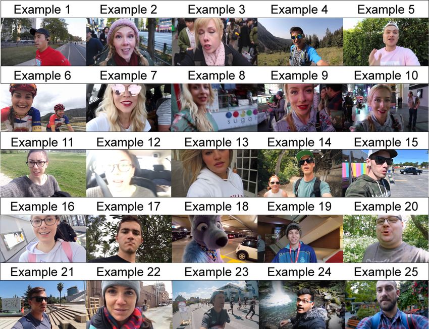
Figure 3. The warping strategy of our method. The background fea-
                                                                      ture points in the same color are in correspondence. The feature
                                                                      points with grid patterns are the warp nodes. The arrows repre-
                                                                      sent the MLS warping operation. During the stabilization, both the
                                                                      feature points Pt (solid blue points) and the face vertices Ft (solid
                                                                      yellow points) are warped by the warp nodes Qt (grid green points).
                                                                      3. Overview of algorithm pipeline
                                                                         Our pipeline is shown in Fig. 2. The pipeline consists of
                                                                      three major parts: motion detection, stabilization and warp-
                                                                      ing. In this section, we will introduce these parts separately
Figure 2. The pipeline of our method. A We first detect the fore-
ground regions of the input video frame. B The background motion
                                                                      and provide an overview of the selfie video stabilization pro-
is tracked using feature points. C The foreground motion is tracked   cess. For completeness, we summarize the notations used in
using 3D face vertices. D We train a stabilization network to infer   our paper and supplementary material in supplementary Ta-
the displacement of the MLS warp nodes. Finally, we use a grid to     ble a. The training of the neural networks mentioned below
approximate the MLS warping and generate the stabilized frame.        will be discussed in Sec. 4.

However, their method uses the optical flow to detect the             3.1. Motion Detection
background motion and the foreground mask, which is com-                  As discussed in Sec. 1, for selfie videos, we seek to stabi-
putationally expensive for real-time applications. Their              lize the foreground and background at the same time. There-
method is also based on global motion optimization, which             fore, both the motion of the face and the background need
makes it impractical in online video stabilization. Our               to be detected. To distinguish the foreground and the back-
method does not require the dense optical flow computation            ground, we first use a pre-trained foreground detection net-
and does not require future motion information, therefore is          work to infer a foreground mask Mt where Mt = 1 rep-
more efficient than their method.                                     resents the foreground region of frame t. We show a sam-
    Steadiface [19] is an online real-time selfie video stabi-        ple foreground mask in Fig. 2 A . The details regarding the
lization method. They used facial key points as the reference         foreground detection network will be discussed in Sec. 4.2.
and the gyroscope information as auxiliary to stabilize hu-           For the background region where Mt = 0, we use the Shi-
man faces. However, their approach uses simple full-frame             Tomasi corner detector[20] to detect feature points in a frame
transformation to warp the frame, which cannot compensate             and the KLT tracker to find their correspondences in the next
for non-linear distortion like rolling shutter. Our method uses       frame, as shown in Fig. 2 B . We uniformly sample 512 fea-
grid-based MLS warping which provides flexibility to handle           ture points for each frame, since fewer feature points can-
non-linear distortions. Our method also models the face mo-           not provide enough coverage of frame regions and more fea-
tion more accurately using a face mesh instead of face land-          ture points will make the pipeline less efficient without sig-
marks in [19]. Due to these limitations, Steadiface [19] will         nificant improvement in warping quality. We will visually
not produce results comparable with ours by simply adding a           compare the different number of feature point selections in
hyperparameter to control foreground and background stabi-            Sec. 6. We denote the selected feature points in frame t as
lization like our method. We will show that the quality of our        Pt ∈ R2×512 . Their correspondences in frame t + 1 are de-
results is significantly better than Steadiface [19] in Fig 10(b)     noted as Qt+1 ∈ R2×512 .
and the supplementary video.                                              To detect the motion of the foreground, we fit a 3D face
    MeshFlow [13] is an online real-time general video stabi-         mesh to each frame using 3DDFA proposed in [26]. An ex-
lization method. They use a sparse grid and feature points            ample of a fitted 3D face mesh is shown in Fig. 2 C . As in the
to estimate the dense optical flow. However, as a general             background, we uniformly sample 512 face vertices to repre-
video stabilization method, they do not consider the fore-            sent the face position in a frame. Furthermore, we only con-
ground/background motion and the large occlusion imposed              sider the 2D projection of the face mesh in our method. In this
by the face and body. This reduces the robustness in the con-         paper, we denote the selected face vertices as Ft ∈ R2×512 ,
text of selfie videos.                                                where t represents the frame index.
    In Sec. 6, we will compare our result with selfie video sta-      3.2. Stabilization
bilization [24], Steadiface [19], MeshFlow [13] and the state-
of-the-art learning based approaches [4, 21]. We also com-               To stabilize the video, we use the rigid moving least
pare with the bundled camera path video stabilization [14]            square(MLS) warping[18] to warp the frames. In Fig. 3, we
representing a typical offline general video stabilization            depict the warping strategy of a video sequence. The mov-
method as the reference.                                              ing least square warping requires a set of warp nodes for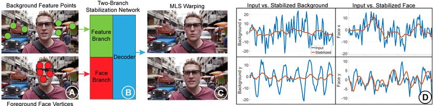
Figure 4. A Our selfie video dataset. From left to right: color frame, ground truth foreground mask, background feature points, 3D face mesh.
B Examples of the foreground mask detected with our trained foreground detection network.

                                                                         4. Network
                                                                             In this section, we discuss the details regarding the stabi-
                                                                         lization network and foreground detection network. We first
                                                                         present our novel selfie video dataset (Sec. 4.1), then discuss
                                                                         details of the foreground detection network (Sec. 4.2) and sta-
                                                                         bilization network (Sec. 4.3). In the supplementary meterial,
                                                                         we introduce a sliding window scheme to apply our stabiliza-
Figure 5. Our stabilization network structure. On the left we show       tion network to arbitrarily long videos (Sec. H.2).
a sequence of input frames. A The feature points and their corre-
spondences in the next frame are concatenated as a 4 × 512 ten-
sor. B The tensors in the same window are concatenated to a large        4.1. Dataset
4(T − 1) × 512 tensor. The same operation is done for face ver-
tices. The output of C the feature branch and D the face branch of           Although large scale video datasets like Youtube-8M [1]
our network are weighted by λ and concatenated. E The decoder
                                                                         have been widely used, public videos with continuous pres-
outputs the displacements of the warp nodes. The layer parameters
are provided in the supplementary material Table b
                                                                         ence of faces are difficult to collect. We propose a novel selfie
                                                                         video dataset containing 1005 selfie video clips, which is sig-
each frame t. We use the correspondences of detected fea-                nificantly larger than existing selfie video datasets proposed
ture points, i.e., Qt , as the warp nodes for frame t (marked            in [24](33 videos) and [9](80 videos). We first manually col-
by gridded green dots in Fig. 3). Besides all the pixels in              lect long vlog videos captured with mobile devices from the
frame t, the feature points Pt (solid blue dots) and the face            Internet. In these videos, we aim to locate the clips that have
vertices Ft (solid yellow dots) are also warped by Qt during             stable face presence. We use the face detector from Dlib [7]
the stabilization to reflect the change of their positions.              to detect faces in each frame, and maintain a global counter to
   Denote the target location of the warp nodes as Q     b t , then      count the number of consecutive frames that contain faces. If
the rigid MLS warping operation (shown as the arrows in                  the face can be detected in more than 50 consecutive frames,
Fig. 3) can be written as a function W (v; Qt , Qb t ), where v is       we cut the raw video into a new clip. In addition to the reg-
a pixel/feature point/face vertex to be warped. Denoting each            ular color videos, our dataset also includes a ground truth
column of a matrix Qt as qi,t ∈ R2×1 where i ∈ [1, 512], the             foreground mask for each frame. We manually label the fore-
rigid MLS warping procedure is defined by a series of com-               ground region of the first frame of each video clip, then use
putations. We included the details of the MLS warping in                 Siammask E [3] to track the foreground object and gener-
supplementary material Algorithm 1. In this paper, we pro-               ate the foreground mask for the video clip. In addition, we
pose a convolutional network (Fig. 2 D ) to infer the displace-          also provide the detected feature points in each frame and
                         b t − Qt . In Sec. 4.3, we will discuss         their correspondences in the next frame. Finally, for each
ments of warp nodes Q
                                                                         frame, we provide the dense 3D face mesh fitted using [26].
the training of this stabilization network.
                                                                         In Fig. 4 A , we show a video still, the corresponding fore-
3.3. Warping                                                             ground mask, the background feature points and the 3D face
                                                                         mesh from our dataset. Our dataset will be made publicly
    More feature points(warp nodes) leads to less warping ar-            available upon publication.
tifacts but longer time to detect and track. In our paper, we
use 512 feature points as warp nodes in each frame, which is
a tradeoff between visual quality and runtime performance.               4.2. Foreground Detection Network
Details will be discussed in supplementary material Sec. J.2.
Although the MLS warping can achieve real-time warping                      Since we have the ground truth mask for our selfie video
with a relatively small number of warp nodes, in our applica-            dataset, training a binary segmentation network is straightfor-
tion, warping with hundreds of warp nodes is both time and               ward. We train an FCN8s network proposed in [16] for this
memory inefficient. With our implementation of GPU accel-                segmentation task. Although there are more advanced struc-
erated MLS warping, with 512 warp nodes, a frame of size                 ture for segmentation [17, 2], we find that FCN8s achieves
448 × 832 must be divided into 16 blocks in order to be fit              satisfactory results for our application. The input of the net-
in a NVIDIA 2080Ti GPU’s memory and the warp speed is                    work is the raw RGB frame, and the output is the binary seg-
approximately 1s/frame. This makes it prohibitive for real-              mentation mask M mentioned in Sec. 3.2. The training uses
time applications. To address this issue, we use a grid to ap-           Adam optimizer with a 10−3 learning rate and a binary cross
proximate the MLS warp field. This approximation enables                 entropy loss. Figure 4 B provides examples of the inferred
real-time performance of our method and yields high-quality              masks on video frames outside our dataset. Note that the in-
visual results. In Sec. 5, we will demonstrate the details of            ferred mask is not perfect, but it is accurate enough to distin-
the grid warping approximation.                                          guish the foreground and the background.
4.3. Stabilization Network                                                 (Figs. 5 C and D ), which only convolve with the last dimen-
                                                                           sion of the tensors. The encoded tensor from different down-
   For a video with T frames, we are able to detect T − 1                  sample levels are weighted by λ and concatenated for skip
groups of feature points Pt and their correspondences in                   connection to decoders (Fig 5 E ), so that the stabilization of
the next frame Qt+1 using the KLT tracking mentioned in                    foreground and background can be controlled by the user in-
Sec. 3.1. For each frame, we seek to infer the displacement                put λ. Note that the order of feature points does not affect the
of warp nodes Qb t −Qt so that the overall motion of the video
                                                                           network, since we train the network with randomly sampled
is minimized. Formally, the loss function for the background               feature points and face vertices and the encoder downsamples
can be written as                                                          the input and essentially blends the feature points regardless
                  T
                  X −1                                                     their original order. The decoder generates the displacements
           Lb =                     b t) − Q
                       W (Pt ; Qt , Q      b t+1            (1)            of the warp nodes. Note that for a length T video, we do not
                                                         2
                    t=1                                                    warp the first frame and last frame. The reason is that the goal
                                                                           of video stabilization is to smooth the original motion, not to
where W (Pt ; Qt , Qb t ) is the MLS warping function as men-              eliminate the motion. Our network is effectively inferring the
tioned in Sec. 3.2. Note that here we apply the MLS warping                warp field for the intermediate T − 2 frames and stabilizes
function to a group of feature points, i.e., each column of Pt             the video instead of aligning all the frames.
are treated as the coordinates of a pixel and warped by all the            Linear Network Design Conventional neural networks con-
warp nodes according to supplementary material Algorithm                   tain activation layers to introduce non-linearity. While we
1. Since the Pt ’s correspondence Qt+1 are the warp nodes                  started with this design, we found, perhaps surprisingly, that
for the next frame, so here we should directly use their new               better performance could be obtained by removing the non-
position Qb t+1 .
                                                                           linearities(supplementary material Table d). Specifically, our
   Similarly, we can also define the foreground loss function              network does not contain activation layers, which is different
using the face vertices:                                                   from conventional neural networks. Intuitively, the definition
          T
          X −1                                                             of the loss function(Eq. 3) requires a linear relationship be-
   Lf =                       b t ) − W (Ft+1 ; Qt+1 , Q
                 W (Ft ; Qt , Q                        b t+1 )       (2)   tween the input and the output of the stabilization network,
                                                                 2
          t=1                                                              i.e. N times larger feature point coordinates require N times
                                                                           larger output displacement that compensates the motion.
 In this equation, the difference with Eq. 1 is that the face
vertices in the next frame t + 1 are warped by the warp nodes                  An obvious question to ask here is why training a network
Qt+1 .                                                                     is necessary to represent the linear relationship. In principle,
   We also introduce a value λ to control the weighting of                 we could pose the problem as an optimization in two alter-
foreground stabilization and background stabilization. The                 native ways. First, it can be modeled as a linear problem in
complete loss function is defined as:                                      which we solve for a matrix that linearly transforms the vec-
                                                                           tor of input feature points into the output displacement vector.
                      L = (1 − λ)Lb + λLf                            (3)   However, this approach leads to an underdetermined problem
                                                                           with too many variables to be solved for in the full matrix.
In Eq. (3), the value λ ∈ (0, 1) controls the stabilization focus          Second, we can use a non-linear solver to directly optimize
on foreground versus background. A larger λ means that we                  the loss function by solving for the output displacement vec-
tend to stabilize the face more, and a smaller λ means we tend             tor. However, this solution is prohibitive due to the runtime
to stabilize the background more. Our method uses λ = 0.3                  performance and result quality.
by default and stabilizes the video automatically. The user                    In the supplementary material, we provide a more thor-
can also change the value online during the stabilization. In              ough analysis of our choice of using a linear network. Briefly,
the supplementary video, we will show an example of our                    the linear neural network factorizes or regularizes the full
network seamlessly changing λ during the stabilization.                    matrix optimization (first alternative solution) into smaller
Network Structure Our network structure is inspired by the                 sub-problems that are easier to solve with fewer variables.
2D autoencoder network structure. However, our formula-                    Specifically, our analysis includes the necessity of using a
tion only provides sparse feature points as 1D vectors. The                network(Sec. I.2), why posing the problem as a non-linear
input dimension does not match the 2D network structure.                   optimization is prohibitive(Sec. I.3) and the performance
Moreover, the vanilla autoencoder structure does not provide               comparison with traditional neural networks(Sec. I.4).
control over the foreground and background stabilization. To
solve these problems, we design our network as a 1D autoen-                Training Our dataset does not contain ground truth
coder with two input branches. We demonstrate our network                  stable videos. Therefore, our training procedure is un-
structure in Fig. 5. For simplicity, we will omit the batch di-            supervised. The goal is to learn to minimize the loss
mension in the discussion. For each frame, the feature points              function defined in Eq. 3, i.e. the distances between feature
Pt ∈ R2×512 and Qt ∈ R2×512 mentioned in Sec. 3.1 are                      points/face vertices detected in consecutive frames. Note that
concatenated in the row dimension, resulting in a frame fea-               the warping is learned solely from groups of unstructured
ture tensor Xt ∈ R4×512 as shown in Fig. 5 A . We con-                     feature points/face vertices. To avoid overfitting, we need
catenate the frame feature tensor of T − 1 frames, forming                 sufficient diversity in the spatial distribution of these points
the feature branch input tensor X ∈ R4(T −1)×512 shown in                  and motion patterns across the frames. Previously discussed
Fig. 5 B . Similarly, we concatenate the face vertices into                efforts we made to satisfy this requirement include a large
the face branch input tensor Y ∈ R4(T −1)×512 . Tensor X                   selfie video dataset(Sec. 4.1) and randomly drawn feature
and Y are encoded separately with 1D convolutional layers                  points/face vertices(Sec. 4.3). In addition, we further perturb
23), crowd (example 2, 3, 9, 10, 16, 23, 24) and wild (exam-
                                                                        ple 4, 5, 6, 11, 14, 17, 20, 24, 25). Some of these videos are
                                                                        selected since their content is technically challenging. These
                                                                        challenges include lack of background features (example 6,
Figure 6. Part of the 25 selfie video examples referred to in Sec. 6.   7, 12, 15), dynamic background (example 2, 3, 9, 10, 16, 23,
Please find complete video stills and corresponding IDs in the sup-     24), sunglasses (example 4, 7, 14, 15, 21), large foreground
plementary material. Our example videos are selected to cover a         occlusion (example 13, 16, 20, 22), face cannot be detected
variety of challenging scenarios in real applications.                  or incomplete face (example 8, 9, 13, 16, 18, 20, 22), multiple
                                                                        faces (example 6, 14) and intense motions (example 1, 23).
the coordinates of feature points/face vertices using a random          Since the dynamics cannot be shown through video stills, we
affine transformation with rotation between [−10◦ , 10◦ ] and           recommend readers to watch our supplementary video. In the
translation between [−50, 50] except the first frame and the            supplementary video, we show the example video clips and
last frame. We also generate a random λ value between                   our stabilized result side by side. As mentioned in Sec. 2, we
(0, 1). We use Adam optimizer with a 10−4 learning rate                 also provide visual and quantitative comparison with the of-
to minimize the loss (Eq. 3) on length T selfie video clips             fline selfie video stabilization [24], the real-time selfie video
randomly drawn from our dataset.                                        stabilization Steadiface [19], the real-time general video sta-
                                                                        bilization MeshFlow [13], the offline general video stabi-
5. Warping Acceleration                                                 lization bundled camera paths [14] and the state-of-the-art
                                                                        learning-based methods [4] and [21]. Since our videos do
    As discussed in Sec. 3, using the MLS warping with 512
                                                                        not contain gyroscope data, we compare with Steadiface [19]
warp nodes in our case is impractical for real-time applica-
                                                                        using only the examples provided in their paper. Apart from
tion. To accelerate the warping speed, for the final rendering
                                                                        the results discussed in this section, we provide more discus-
of the frame, we use a grid to approximate the warp field gen-
                                                                        sion regarding the number of feature points(warp nodes) in
erated by MLS warping. Denote a grid vertex in frame t by
                                                                        supplementary Sec. J.2, ablation study regarding the FG/BG
gj ∈ R2×1 , where j is the index of grid vertices. Each pixel
                                                                        mask in supplementary Sec. J.3 and performance with differ-
v can be defined by the bilinear interpolation of the enclosing
                                                                        ent input resolution in supplementary Sec. J.4.
four grid vertices, denoted by G ∈ R2×4 : v = GD, where
D ∈ R4×1 is the vector of bilinear weights.                             6.1. Value of λ
    In the first step of rendering, we warp the grid vertices
with warp nodes Qt and their target coordinates Q    b t: g
                                                          bj =             In Fig. 7 we show the effect of different values of λ. We
                                                                        stabilize the same video clip with λ set to 0.3 and 0.9 respec-
W (gj ; Qt , Qt ). Since the grid vertices are sparse, warp-
             b
                                                                        tively. To show the steadiness of the result, we average 15
ing with MLS is computationally efficient. We then densely              consecutive frames of the stabilized video. The less blurry
warp the pixels v using the MLS warped grid coordinates:                the region is, the more stable it is in the result. For λ = 0.9,
v
b = GD, b     where G b consists of the transformed enclosing           the face regions are less blurry as shown in the green inset,
four grid vertices gbj . This step contains only one matrix op-         indicating that our network automatically focuses on stabiliz-
eration, which can be computed at a real-time rate. In our              ing the face. If we set λ = 0.3, the background regions are
experiment, we find the difference between the results gener-           less blurry as shown in the cyan inset meaning that the back-
ated with the dense MLS warping and grid approximation is               ground is more stable. In our experiment, we use a default
negligible. Our method is not sensitive to the selection of the         value of λ = 0.3, meaning that we stabilize both foreground
grid size. In our experiment, we use a grid size 20 × 20. We            and background while mainly focusing on the background.
implemented the grid warping on GPU by parallel sampling
the grid with a pixel-wise dense grid, generating a dense warp          6.2. Visual Comparison
field. We then use the dense warp field to sample the video
                                                                            We show sample frames from our examples and the sta-
frame, generating the warped frame. Our implementation of
                                                                        bilized results in Fig. 8. Our method stabilizes the frames
this process takes approximately 4ms/frame, compared to the
                                                                        without introducing visual distortions. The real-time general
1s/frame ground truth dense MLS warping.
                                                                        video stabilization method [13] and offline general video sta-
6. Results                                                              bilization method [14] usually produce artifacts on the face,
                                                                        since they do not distinguish the foreground and the back-
   In this section, we present the results of our method. Note          ground. Selfie videos are also challenging for the optical flow
that our dataset is cut from a small number of long vlog                estimation in MeshFlow [13], since the motion within a mesh
videos, therefore the faces are from a limited number of peo-           cell can be significantly different due to the foreground oc-
ple. Some videos in our dataset also do not actually need to be         clusion. The learning based method [21] generally does not
stabilized (e.g., still camera video). To show the effectiveness        produce local distortions, but tends to generate unstable out-
and the ability of generalization of our method, we collect 25          put video. Due to the accuracy issue in optical flow and frame
new selfie videos that contain a variety of challenging sce-            interpolation, the other learning based method [4] generates
narios in real applications, and are completely separate from           artifacts, especially near the occlusion boundaries like face
our training dataset. Part of the testing examples are shown            boundaries. These artifacts are more obvious when observed
in Fig. S3. The complete example video stills with video IDs            dynamically in videos. We recommend the readers to watch
will be provided in supplementary Fig. S3. The background               the supplementary video for better visual comparison. We
scenes vary from indoor (example 16, 18, 19), inside of cars            also achieve the same quality visual results as the previous
(example 7, 12), city (example 1, 2, 8, 9, 10, 13, 15, 21, 22,          optimization based selfie video stabilization [24]. However,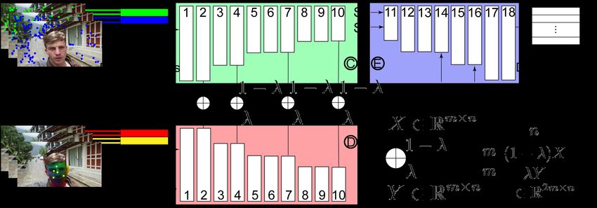
Figure 7. The visual comparison of different values of λ in our method and the state-of-the-art real-time face stabilizaiton method Steadi-
face [19] using the example videos provided in their work. The images shown are the average of 15 consecutive frames. The face regions and
the background regions of the input, the corresponding regions of Steadiface [19] and our method are shown in the insets on the right.
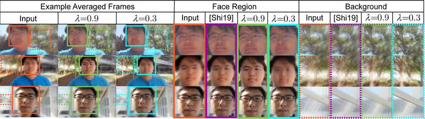
Figure 8. The visual comparison of bundled camera paths [14], selfie video stabilization [24], MeshFlow [13], deep online video stabiliza-
tion [21], deep iterative frame interpolation [4] and our method. The details of the face regions are shown in the insets on the right. We
recommend readers to zoom in and observe the details in the images.
6.3. Quantitative comparison
We use the three quantitative metrics proposed in [14] to
evaluate the frame size preservation (Cropping), visual dis-
tortion (Distortion) and steadiness (Stability) of the stabiliza-
tion result. Note that since Steadiface [19] require gyroscope
Figure 9. Quantitative comparison of bundled camera paths [14], information to stabilize the video, the quantitative compar-
selfie video stabilization [24], MeshFlow [13], deep online video ison with their method is conducted using their videos and
stabilization [21], deep iterative frame interpolation [4] and our will be discussed in Fig. 10 B .
method. In these metrics, a larger value indicates a better result. In the left column of Fig. S2, we show the cropping metric
The average values over all the example videos are listed. The com- comparison. A larger value represents a larger frame size of
plete comparison on individual videos are provided in the supple- the stabilized result. Although [24] uses second order deriva-
mentary material Fig. S2. tive objective, their frame size is limited by the motion of the
our method is learning-based and runs at the real-time speed, entire video. Our sliding window only warps the frames with
which is orders of magnitude faster compared to their method respect to the temporally local motion, so we are still able to
as we will discuss in Sec. 6.4. achieve similar cropping value while directly using the ex-
We also test our method on the examples in Steadi- plicit motion loss in Eq. (3). The frame size of our result is
face [19], which is the state-of-the-art real-time face stabi- also significantly greater than [13], [21] and [14], since the
lization method. The images shown on the left of Fig. 7 are artifacts in their results often cause over-cropping in the final
the average consecutive 15 frames of their results. If we set video. Since [4] is based on frame interpolation, their crop-
λ = 0.9 in our method (mainly stabilize the face), we are able ping score is by default equal to 1. However, [4] is essentially
to achieve better face alignment. In addition, we can alterna- an offline method requiring multiple iterations over the entire
tively set λ = 0.3 in the stabilization network. The back- video. In the following discussions, we will show that their
ground becomes significantly more stable than the Steadi- distortion and stability score is much worse than ours.
face [19] results and our λ = 0.9 results in the averaged In the middle column of Fig. S2, we show the distortion
frames, indicating that our method is capable of stabilizing metric. This metric measures the anisotropic scaling of the
the background. Figure 7 also indicates that stabilizing the stabilized frame. A larger value indicates that the visual
background (λ = 0.3) leads to a slight sacrifice of face sta- appearance of the result is more similar to the input video.
bility, since the motion of the foreground and background is Since we warp the frame with grid approximated moving
different. In our supplementary video, we will show that this least squares, minimal anisotropic scale was introduced to
loss of face stability is visually unnoticeable. the result. The MeshFlow method [13] and bundled cam-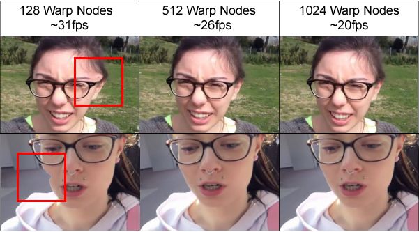
frames and multiple iterations through the entire video.
                                                                          Although our method is slightly slower than Mesh-
                                                                      Flow [13] and deep multi-grid warping [21], we have shown
                                                                      in Sec. 6.2, Sec. 6.3 and supplementary video that our method
                                                                      produces significantly better results than theirs. Our method
                                                                      is also slower than Steadiface [19]. However, our method is
Figure 10. Quantitative comparison with A selfie video stabiliza-     a purely software video stabilization and requires no gyro-
tion [24] and B Steadiface [19] using their datasets respectively.    scope information, which is not available on some devices,
The average values over the entire datasets are plotted. In all the   e.g., action cameras. In addition, since gyroscope informa-
three metrics, a larger value indicates a better result.              tion does not provide direct image domain motion, our ap-
era paths [14] introduces unexpected local distortion to the          proach usually yields visually more stable results as we will
frame, which leads to the negative impact on the distortion           show in our supplementary video. As we discussed earlier
value. The learning based methods [21] and [4] cannot gen-            in Sec. 2, our method essentially more accurately models the
eralize to selfie videos. They also produce visual artifacts that     frame motion than Steadiface [19]. Therefore their method
lead to even worse distortion values comparing to optimiza-           does not generate comparable quality as our method. Also
tion based methods [13, 14].                                          note that our method also runs at a real-time speed without
   The right column of Fig. S2 shows the stability metric             any attempt to optimize the implementation. We believe that
comparison. A larger stability metric indicates a more stable         the speed of our pipeline can be further improved by using
result. This is the most important metric for video stabiliza-        the GPU memory sharing between feature detection/tracking
tion. Comparing with the input (the yellow bar on the left of         and neural network operations to avoid repetitive data trans-
each example), our method significantly increases the stabil-         ferring between CPU and GPU.
ity in the result. Our method achieves a comparable result
with the optimization based method [24] with orders of mag-           6.5. Limitation
nitude improvement in stabilization speed. We also achieve
better stability than [4, 13, 14, 21], which is expected since           Our method fails if very few feature points are detected
their visual result is not satisfactory as shown in Fig. 8.           in the background, since our method requires a reasonable
   To further verify the performance of our method, we also           number of warp nodes to warp the frame. These cases in-
test our method on the selfie videos provided in [24] and [19].       clude very dark environments, pure white walls and blue sky.
Figure 10 shows the average values of the three metrics above         This is a common limitation for feature tracking based meth-
on the selfie video dataset proposed by A [24] and B [19].            ods [5, 6, 10, 11, 14]. In our method, this can be solved by
Again, our result has a quantitative performance comparable           replacing the feature tracking with the optical flow algorithm
with [24]. Our method also performs better than [19] without          with appropriate accuracy and real-time performance.
using the gyroscope information.
6.4. Stabilization Speed
                                                                      7. Conclusions and Future Work
    Our code is written in Python and runs on a desktop com-              In this paper, we proposed a real-time learning based selfie
puter with an NVIDIA 2080Ti graphics card. On average, our            video stabilization method that stabilizes the foreground and
method uses 38ms to stabilize a frame of resolution 832x448,          background at the same time. Our method uses the face mesh
which is equivalent to 26fps. The break down of runtime is            vertices to represent the motion of the foreground and the 2D
3ms for foreground mask detection, 7ms for the feature detec-         feature points as the means of background motion detection
tor, 3ms for KLT tracking, 16ms for face mesh detection, 5ms          and the warp nodes of the MLS warping. We designed a two
for stabilization network inference, less than 1ms for MLS            branch 1D linear convolutional neural network that directly
grid approximation and 4ms for frame warping. For other               infers the warp nodes displacement from the feature points
video resolutions, we rescale the feature points to match our         and face vertices. We also propose a grid approximation to
frame size of 832x448. The only operation impacted is the             the dense moving least squares that enables our method to
grid warping. However, since the warping is implemented on            run at a real-time rate. Our method generates both visually
the GPU, the difference is subtle, e.g. 4ms for HD(1280x720)          and quantitatively better results than previous real-time gen-
and 6ms for FHD(1920x1080). The overall speed is around               eral video stabilization methods and comparable results to the
40ms/frame for HD and 42ms/frame for FHD. With frame                  previous selfie video stabilization method with a speed im-
size 832x448, the average stabilization time of the compar-           provement of orders of magnitude.
ison methods(per frame) are: 4720ms for selfie video sta-                 Our work opens up the door to high-quality real-time sta-
bilization [24], 392ms for bundled camera paths[14], 8ms              bilization of selfie videos on mobile devices. Moreover, we
for Steadiface[19], 20ms for MeshFlow[13], 28ms for deep              believe that our selfie video dataset will inspire and provide a
online video stabilization[21], 67ms for deep iterative frame         platform for a variety of graphics and vision research related
interpolation[4]. Our method is nearly two orders of magni-           to face modeling and video processing. In the future, we
tude faster than the previous selfie video stabilization [24],        would explore the possibility of learning based selfie video
and nearly an order of magnitude faster than the traditional          frame completion using our proposed selfie video dataset.
optimization based general video stabilization [14]. Our              Acknowledgements. This work was funded by a Qualcomm
method is also nearly two times faster than the frame interpo-        FMA Fellowship. We also acknowledge support from the
lation method [4], since their network involves 2D convolu-           Ronald L. Graham chair and the UC San Diego Center for
tions. Also note that [4] is an offline method requiring future       Visual Computing.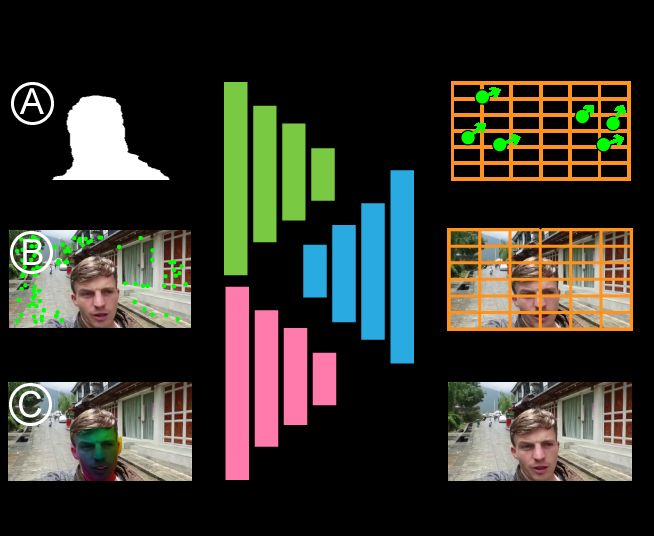
References                                                            [21] M. Wang, G. Yang, J. Lin, S. Zhang, A. Shamir, S. Lu, and S.
                                                                           Hu. Deep online video stabilization with multi-grid warping
 [1] Sami Abu-El-Haija, Nisarg Kothari, Joonseok Lee, Apos-                transformation learning. IEEE Transactions on Image Pro-
     tol (Paul) Natsev, George Toderici, Balakrishnan Varadarajan,         cessing, 28(5):2283–2292, 2019.
     and Sudheendra Vijayanarasimhan. Youtube-8m: A large-
     scale video classification benchmark. In arXiv:1609.08675,
     2016.
 [2] P. Chao, C. Kao, Y. Ruan, C. Huang, and Y. Lin. Hardnet: A
     low memory traffic network. In IEEE International Confer-
     ence on Computer Vision (ICCV), 2019.
 [3] Bao Xin Chen and John K Tsotsos. Fast visual object tracking     [22] Yu-Shuen Wang, Feng Liu, Pu-Sheng Hsu, and Tong-Yee Lee.
     with rotated bounding boxes. In arXiv:1907.03892, 2019.               Spatially and temporally optimized video stabilization. IEEE
 [4] Jinsoo Choi and In So Kweon. Deep iterative frame interpo-            Trans. Visual. and Comput. Graph., 19(8), Aug 2013.
     lation for full-frame video stabilization. ACM Trans. Graph.,
     39(1), Jan. 2020.
 [5] Amit Goldstein and Raanan Fattal. Video stabilization using
     epipolar geometry. ACM Trans. Graph., 31(5), Sept. 2012.
 [6] Matthias Grundmann, Vivek Kwatra, and Irfan Essa. Auto-
     directed video stabilization with robust l1 optimal camera
     paths. In The IEEE Conference on Computer Vision and Pat-        [23] Sen-Zhe Xu, Jun Hu, Miao Wang, Tai-Jiang Mu, and Shi-Min
     tern Recognition (CVPR), 2011.                                        Hu. Deep Video Stabilization Using Adversarial Networks.
                                                                           Computer Graphics Forum, 2018.
 [7] Davis E. King. Dlib-ml: A machine learning toolkit. Journal
     of Machine Learning Research, 10:1755–1758, 2009.
 [8] V. Lempitsky, A. Vedaldi, and D. Ulyanov. Deep image prior.
     In The IEEE Conference on Computer Vision and Pattern
     Recognition (CVPR), 2018.
 [9] Yiming Lin, Shiyang Cheng, Jie Shen, and Maja Pantic. Mob-
     iface: A novel dataset for mobile face tracking in the wild.     [24] Jiyang Yu and Ravi Ramamoorthi. Selfie video stabilization.
     In The IEEE International Conference on Automatic Face and            In European Conference on Computer Vision (ECCV), 2018.
     Gesture Recognition (FG), 2019.
[10] Feng Liu, Michael Gleicher, Hailin Jin, and Aseem Agarwala.
     Content-preserving warps for 3D video stabilization. ACM
     Trans. Graph., 28(3), July 2009.
[11] Feng Liu, Michael Gleicher, Jue Wang, Hailin Jin, and Aseem
     Agarwala. Subspace video stabilization. ACM Trans. Graph.,
     30(1), Feb. 2011.                                                [25] Jiyang Yu and Ravi Ramamoorthi. Robust video stabilization
[12] S. Liu, M. Li, S. Zhu, and B. Zeng. Codingflow: Enable video          by optimization in cnn weight space. In The IEEE Conference
     coding for video stabilization. IEEE Transactions on Image            on Computer Vision and Pattern Recognition (CVPR), 2019.
     Processing, 26(7):3291–3302, 2017.
[13] Shuaicheng Liu, Ping Tan, Lu Yuan, Jian Sun, and Bing Zeng.
     Meshflow: Minimum latency online video stabilization. In
     European Conference on Computer Vision (ECCV), 2016.
[14] Shuaicheng Liu, Lu Yuan, Ping Tan, and Jian Sun. Bundled
     camera paths for video stabilization. ACM Trans. Graph.,
                                                                      [26] Xiangyu Zhu, Xiaoming Liu, Zhen Lei, and Stan Z Li. Face
     32(4), July 2013.
                                                                           alignment in full pose range: A 3d total solution. IEEE Trans-
[15] Shuaicheng Liu, Lu Yuan, Ping Tan, and Jian Sun. Steadyflow:          actions on Pattern Analysis and Machine Intelligence, 41(1),
     Spatially smooth optical flow for video stabilization. In The         2019.
     IEEE Conference on Computer Vision and Pattern Recognition
     (CVPR), 2014.
[16] J. Long, E. Shelhamer, and T. Darrell. Fully convolutional
     networks for semantic segmentation. In IEEE Conference on
     Computer Vision and Pattern Recognition (CVPR), 2015.
[17] V. Nekrasov, Chunhua Shen, and I. Reid. Light-weight re-
     finenet for real-time semantic segmentation. In The British
     Machine Vision Conference (BMVC), 2018.
[18] Scott Schaefer, Travis McPhail, and Joe Warren. Image de-
     formation using moving least squares. ACM Trans. Graph.,
     25(3), July 2006.
[19] Fuhao Shi, Sung-Fang Tsai, Youyou Wang, and Chia-Kai
     Liang. Steadiface: Real-time face-centric stabilization on mo-
     bile phones. In IEEE International Conference on Image Pro-
     cessing (ICIP), 2019.
[20] Jianbo Shi and Carlo Tomasi. Good features to track. In The
     IEEE Conference on Computer Vision and Pattern Recognition
     (CVPR), 1994.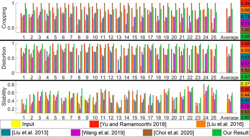
Supplementary Material

   Table a. Notations in the paper and supplementary material
 Symbols           Explanation
 t                 Frame index
 Mt                Foreground mask
 Pt                Background feature points
 Qt                Correspondence of Pt−1 in frame t
 Ft                Face vertices
 Q
 bt                Target coordinate of Qt
 v                 Coordinate of a pixel
 W (v; Qt , Q
            b t)   Rigid MLS warping function
 v
 b                 Warped coordinate of pixel v
 qi                ith column of Qt
 wi                MLS weight of qi,t to pixel v                Figure S1. The sliding window scheme of our method. The inputs of
                                                                our network for each window are marked with the same color. For
 α                 MLS parameter
                                                                each window, the second frame is stabilized. The background fea-
 c                 Weighted centroid of Qt                      ture points and the foreground face vertices are updated accordingly
 c
 b                 Weighted centroid of Qbt                     and become the next window’s input.
 q∗i               Vector from c to qi,t
 b∗i
 q                 Vector from bc to q
                                     bi
 Ai                Transformation matrix of qb∗i
 gj                jth grid vertex                              MLS warping process referred in Sec. 3.2. Since the MLS
 G                 Grid vertices enclosing v                    warping is not related to the time dimension, we omit the time
 D                 Bilinear weights of v with respect to G      subscript t for simplicity. In Algorithm 1, we use relatively
                                                                small α = 0.3 to maintain a smooth warp field and avoid
 Algorithm 1: The rigid MLS warping algorithm
                                                                artifacts.
 W (v; Q, Q)
          b
  Input : Source coordinates of a pixel v, source node
           coordinates Q and target node coordinates
                                                                H.2. Sliding Window
           Q
           b
  Output: Target coordinates of a pixel v
                                                                    Since the stabilization network only takes fixed length
                                        b
  for i ← 1 to 512 do
                         2α                                     video segments, to apply to arbitrary length selfie videos, we
      wi = 1/ |v − qi |                                         apply a sliding window scheme. In our experiment, we use
  end                 P                                     a sliding window with length T = 5. We demonstrate our
        P512                512
  c=      i=1  wi q i  /    i=1 w i                             sliding window scheme in Fig. S1. Each window is marked
        P
            512
                        P
                             512
                                                               by the same color, which is the input to our network for the
   c=
   b        i=1 wi qi /
                   b         i=1 wi                             window. Consider window 1 as an example. The outputs of
  for i ← 1 to 512 do                                           our stabilization network are the displacements of the warp
      q∗i = (qi − c)T q b∗i = (b     c)T
                                qi − b                          nodes Q b 2, Q
                                                                             b 3 and Q
                                                                                     b 4 as we discussed in the network struc-
                 q∗                                             ture. At this point, if we warp all these frames in the cur-
      Ai = wi −qi∗ ⊥ v − c − (v − c)⊥ ,

                   i                                            rent window and set the next window starting from frame 5,
      where ⊥ is an operator on 2D vector                       the result will be smooth within each window but not glob-
        (x, y)⊥ = (−y, x)                                       ally smooth. Therefore, we only warp the second frame in
  end          P             P                                the current window and shift one frame for the next window.
                   512             512
  b = |v − c|
  v                       b∗i /
                   i=1 Ai q               b∗i + b
                                   i=1 Ai q     c               This scheme ensures temporal consistency between consecu-
                                                                tive windows. Specifically, in this example, we use the MLS
                                                                warp function W (v; Q2 , Q b 2 ) to warp frame 2. We then warp
                                                                the feature points and face vertices using W (P1 ; Q1 , Q  b 1)
H. Implementation Details                                       and W (F1 ; Q1 , Q1 ), since warping the frame leads to up-
                                                                                   b
H.1. MLS warping process                                        dated positions of the original feature points and face ver-
                                                                tices. The updated feature points and face vertices become a
   Table a summarizes the notations used in the main paper      part of window 2, which is the next window starting at frame
and this supplementary material. Algorithm 1 provides the       2.
Table b. Network parameters in main paper Fig. 5 Table c. Linear Network vs. Direct Optimization
Layer Layer Input Size Output Kernel Stride Dilation Padding Methods Cropping Distortion Stability
id Type Size Size Direct Optimization 0.91 0.93 0.40
1 Conv1d 4(T-1)x512 Cx512 3 1 1 1
2 Conv1d Cx512 2Cx256 4 2 1 1 Our Linear Network 0.88 0.97 0.60
3 Conv1d 2Cx256 2Cx256 3 1 1 1
4 Conv1d 2Cx256 4Cx128 4 2 1 1 Table d. Quantitative results from different network designs. In this
5 Conv1d 4Cx128 4Cx128 3 1 1 1 table, C is the number of filters in the first layer of our network
6 Conv1d 4Cx128 4Cx128 3 1 1 1 depicted in Fig. 5
7 Conv1d 4Cx128 8Cx64 4 2 1 1
8 Conv1d 8Cx64 8Cx64 3 1 1 1
9 Conv1d 8Cx64 8Cx64 3 1 2 2 C=32 Cropping Distortion Stability
10 Conv1d 8Cx64 8Cx64 3 1 2 2 No activation 0.85 0.95 0.56
11 ConvT1d 32Cx64 8Cx128 4 2 2 2 Leaky ReLU 0.90 0.97 0.48
12 Conv1d 8Cx128 8Cx128 3 1 1 1
13 Conv1d 8Cx128 8Cx128 3 1 1 1
Tanh 0.87 0.97 0.50
14 ConvT1d 16Cx128 4Cx256 4 2 1 1
15 Conv1d 4Cx256 4Cx256 3 1 1 1 C=64 Cropping Distortion Stability
16 ConvT1d 8Cx256 2Cx512 4 2 1 1 No activation 0.86 0.96 0.57
17 Conv1d 2Cx512 2Cx512 3 1 1 1
18 Conv1d 2Cx512 2(T-2)x512 1 1 1 0
Leaky ReLU 0.92 0.98 0.52
Tanh 0.85 0.96 0.52
I. Network Design C=128 Cropping Distortion Stability
No activation 0.88 0.97 0.60
In this section, we extend the discussion regarding the lin- Leaky ReLU 0.91 0.97 0.57
ear network design. We first provide the complete list of pa- Tanh 0.89 0.96 0.52
rameters in the stabilization network in Sec. I.1. We then
discuss the necessity of using a network instead of formulat-
ing a linear optimization problem in Sec. I.2. In Sec. I.3, we
compare the performance of linear network and direct opti- non-linear moving least squares warping; the problem cannot
mization of the loss function(Eq. 3). In Sec. I.4, we com- be solved using a simple linear system solver as in the bun-
pare the performance of linear network and non-linear net- dled camera paths [14]. Finally, the problem has to be solved
work in terms of the quantitative metrics discussed in main for each sliding window in the online video stabilization,
paper Sec. 6.3. Finally, we compare the performance using making it impossible to achieve real-time performance. On
different number of filters in the network in Sec. I.5. the other hand, the linear neural network has two advantages
I.1. Network Parameters compared to posing the problem as an optimization. First,
the convolutional layers contain only small kernels; the con-
Table b lists the network parameters in main paper Fig. 5. catenation of layers is equivalent to decomposing the dense
The number of filters in each layer is multiple of a base num- matrix into a series of sparse matrices which is easier to solve
ber C, which will be discussed in Sec. I.5 in this supplemen- through backpropagation and gradient descent. Second, the
tary material. network implicitly provides regularization by training on a
large dataset; using a pretrained network avoids the overfit-
I.2. Necessity of the linear network ting problem in the optimization and also enables computa-
In Eq. (1) and Eq. (2) in the main paper, we define the tional real-time performance.
loss function directly on feature points detected in the im-
age. This requires linear relationship between the input and I.3. Direct optimization
the output of the stabilization network, i.e. scaling of fea- Since our network is linear, an obvious question is whether
ture point coordinates should lead to the same scaling of we need a convolutional network at all. A way to pose the
the output displacement to compensate the motion. Note stabilization process as an optimization problem is to directly
that this linear relationship between input and output can solve for the warp node displacement Q b t − Qt to minimize
be posed as a matrix-vector product, i.e., n = Am where the non-linear loss function L. Note that the objective func-
A ∈ R1024(T −1)×4096(T −1) is a large matrix that transforms tion L is non-linear, so a simple least squares linear solver
concatenated and reshaped input feature points and face ver- such as in bundled camera paths [14] cannot be used. We
tices m ∈ R4096(T −1)×1 to reshaped warp node displace- conduct an experiment in which we optimize our loss func-
ments n ∈ R1024(T −1)×1 . The optimization problem equiva- tion Eq. 3 in the main paper directly over the feature points
lent to our network training can be defined as: (warp nodes) instead of network weights. We optimize 1000
iterations using Adam optimizer with lr = 10−1 , β1 = 0.9
min L(m, n), (S1) and β2 = 0.99 for each 5-frame sliding window. Note that
A
although this formulation is tractable comparing to Sec. I.2,
where L is the loss function defined in Eq. 3 in the main the runtime of this optimization is prohibitive for pratical use
paper. Solving this problem directly is difficult and pro- since it requires an average of 20 seconds to stabilize each
hibitive in the video stabilization for the following reasons. frame. We show the quantitative comparison of this optimiza-
First, the matrix A is dense and the problem is highly under- tion result with the result generated by our linear network in
determined. Second, the loss function we defined involves Table c. Although our network is linear, it performs signifi-You can also read