Direct Position-Based Solver for Stiff Rods - Visual Computing Institute
←
→
Page content transcription
If your browser does not render page correctly, please read the page content below
Volume 0 (1981), Number 0 pp. 1–12                                                                                    COMPUTER GRAPHICS forum

                                   Direct Position-Based Solver for Stiff Rods

                                               Crispin Deul1 , Tassilo Kugelstadt2 , Marcel Weiler1 and Jan Bender2
                                                                       1 Graduate School CE, TU Darmstadt
                                                                           2   RWTH Aachen University

Figure 1: Left: The Slinky model shows the performance of our solver in presence of a high number of collisions and self-collisions. Right:
Our method is able to simulate tree-like structures. The white birch model represents a typical deciduous tree.

        Abstract
        In this paper, we present a novel direct solver for the efficient simulation of stiff, inextensible elastic rods within the Position-
        Based Dynamics (PBD) framework. It is based on the XPBD algorithm, which extends PBD to simulate elastic objects with
        physically meaningful material parameters. XPBD approximates an implicit Euler integration and solves the system of non-
        linear equations using a non-linear Gauss-Seidel solver. However, this solver requires many iterations to converge for complex
        models and if convergence is not reached, the material becomes too soft. In contrast we use Newton iterations in combination
        with our direct solver to solve the non-linear equations which significantly improves convergence by solving all constraints
        of an acyclic structure (tree), simultaneously. Our solver only requires a few Newton iterations to achieve high stiffness and
        inextensibility. We model inextensible rods and trees using rigid segments connected by constraints. Bending and twisting
        constraints are derived from the well-established Cosserat model. The high performance of our solver is demonstrated in
        highly realistic simulations of rods consisting of multiple ten-thousand segments. In summary, our method allows the efficient
        simulation of stiff rods in the Position-Based Dynamics framework with a speedup of two orders of magnitude compared to the
        original XPBD approach.
        CCS Concepts
        •Computing methodologies → Physical simulation;

 c 2018 The Author(s)
Computer Graphics Forum c 2018 The Eurographics Association and John
Wiley & Sons Ltd. Published by John Wiley & Sons Ltd.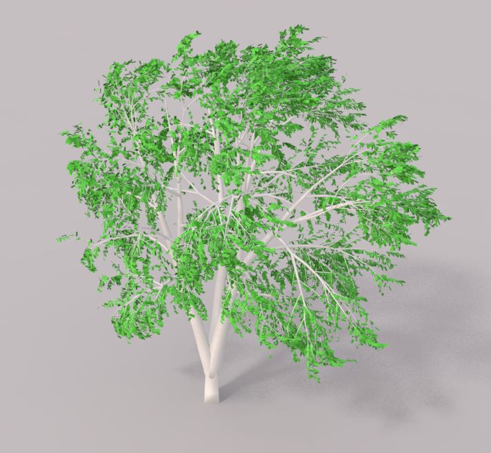
Deul et al. / Direct Position-Based Solver for Stiff Rods

1. Introduction                                                                 ence each other through an immediate position update of the con-
                                                                                strained generalized coordinates. As such, constraint corrections
The simulation of slender, rod-like structures has been an active re-
                                                                                travel only locally from constraint to constraint. Thus, in case of
search area in computer graphics over the last decades and is still
                                                                                a chain of constraints (e.g. a rod) the solver needs many iterations
of high interest. There are various applications like the simulation
                                                                                to converge. However, the system for a single rod does not include
of ropes, threads, hair and fur of virtual characters as well as veg-
                                                                                inequalities. Therefore, in contrast to the original XPBD approach,
etation like trees or other plants. Such models are used for special
                                                                                we solve this system with Newton’s method, where the solution to
effects in movies and in interactive virtual environments like games
                                                                                the subproblems is solved with a linear-time solver. This increases
or surgical simulations. Recently, several methods for the fast and
                                                                                convergence significantly.
stable simulation of elastic rods have been developed. However, the
stable and interactive simulation of very stiff objects like a trunk or            Furthermore, we employ the physically accurate Cosserat rod
branches of a tree, which are very common in nature and every-day               model to achieve realistic bending and torsion resistance. We show
life, remains a challenging problem.                                            how to discretize inextensible and unshearable rods as chains of
                                                                                rigid segments that are connected by a combination of zero-stretch,
    Many real world materials like wood and hair are nearly inex-
                                                                                bending and twisting constraints.
tensible and they can have a large spectrum of bending and tor-
sion resistance. This poses high demands on the numerical inte-                    Our method provides a significant speedup of two orders of mag-
grator. Simple explicit methods require very small time steps to                nitude compared to the non-linear Gauss-Seidel solver. Thus, it
remain stable, which leads to high computational costs. Further-                greatly reduces the time taken to realistically simulate complex
more, numerical stability cannot be guaranteed, but this is crucial             scenes with rods consisting of several ten-thousands rigid segments
in many interactive applications. Lately, Position-based dynamics               and very high bending and torsion stiffness in the Position-based
(PBD) [BMM14] has become very popular, because it is simple to                  dynamics framework. The material stiffness of the tree in Figure 1
implement, numerically stable and very versatile, while it can han-             can be easily tuned by using Young’s modulus and torsion modulus
dle arbitrary position-based constraints. A major problem of PBD                and it realistically depends on the varying thickness of the trunk
is that material stiffness depends on the number of iterations and on           and the branches by using the Cosserat model. The Slinky scene
the time step size. Recently, Macklin et al. [MMC16] published an               shows that collisions are naturally handled by constraints (see Sec-
extended version of PBD, called XPBD, that solved this problem                  tion 4). Moreover, we compared our model to the analytic solution
and supports physically meaningful material parameters. However,                of the bending of a cantilever beam that was fixed at one end that
when it comes to simulations of very large and stiff structures with            demonstrates the accuracy of our method (see Section 5). Finally,
thousands of segments and constraints like the tree in Figure 1, the            our method is easy to implement and can be easily integrated into
solver of XPBD requires a large number of iterations to converge.               existing Position-based dynamics frameworks.
Moreover, the material becomes softer, when too few iterations are
used.
   In this paper we address the convergence problem of iterative                2. Related Work
solvers for rod simulations by exploiting their special acyclic struc-          In this section we discuss the most closely related work in strand
ture (in the rest of the paper called tree). This structure allows for          and rod simulation as well as Position-based dynamics. Many ap-
using a direct solver with linear-time complexity to solve all con-             proaches for the simulation of elastic rods or strands have been
straints in the tree simultaneously. Baraff [Bar96] proposed such a             proposed in computer graphics, including mass spring models,
solver for trees of articulated rigid bodies. More recent works, e.g.           Cosserat models, multi-body strands and position-based methods.
of Hernandez et al. [HGCO11] or Aubry and Xian [AX15], solved
the drift problem of Baraff’s method (c.f. [BET14]) by formulat-
                                                                                Mass spring models: Mass spring models are very popular in
ing implicit position constraints at the end of the time step. Nev-
                                                                                computer graphics due to their simplicity and computational perfor-
ertheless, a rod modeled with one of these approaches might suf-
                                                                                mance and are widely used in cloth and strand simulation [BW98,
fer from jitter in high tension cases [GHF∗ 07, TNGF15]. Han and
                                                                                CCK05, IMP∗ 13]. However, mass spring models cannot naturally
Harada [HH13] proposed a linear time algorithm for particle dis-
                                                                                handle torsion effects of rods. Therefore, Selle et al. [SLF08] used
tance constraints with PBD. However, they only support distance
                                                                                additional altitude springs for the simulation of curly hair. But these
constraints and no elastic potentials and only handle linear chains
                                                                                springs lead to increased computational costs. Another problem is
and no trees.
                                                                                that the only material parameters of mass spring models are the
   The position-based approach avoids the numerical drift problem               stiffness constants of the springs. Therefore, tuning the material
by solving the time integration with an implicit constraint evalu-              behavior is difficult. Michels et al. [MMS15] solved this issue by
ation. Moreover, the discretization with an implicit constraint di-             using special cuboidal mass spring elements for the discretization
rection (ICD) reduces instabilities in tension situations (see Gold-            of the rod. These elements allow the mapping of real world ma-
enthal et al. [GHF∗ 07]). In general, the constraint formulations of            terial parameters like the Young’s or torsion modulus to the spring
XPBD lead to a non-linear system with equalities and inequalities.              constants. Yet their employed exponential integrator makes it math-
The system is not easy to solve and needs special treatment. There-             ematically unclear how hard constraints and non-smooth contacts
fore, XPBD applies a non-linear Gauss-Seidel solver. This solver                are handled. They also report that practical time step sizes for their
computes individual Newton steps for each position constraint in an             simulations are in the range of 10−3 s, while our method runs well
iterative process. The individual solutions of the constraints influ-           for step sizes larger than 10−2 s for similarly sized objects.

                                                                                                                                                    c 2018 The Author(s)
                                                                                   Computer Graphics Forum c 2018 The Eurographics Association and John Wiley & Sons Ltd.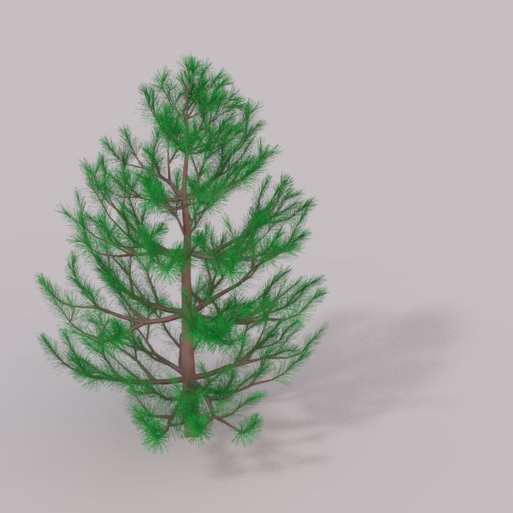
Deul et al. / Direct Position-Based Solver for Stiff Rods

Cosserat rods (implicit discretization): The Cosserat model de-                              frame is sufficient to describe the frame. The reference frames
scribes elastic rods which can undergo stretch, shear, bend and twist                        are constructed by parallelly transporting the reference frame
deformations. An introduction to the Cosserat theory can be found                            from one end along the rod. This construction leads to dense
in the book of Antman [Ant05]. Pai [Pai02] introduced the Cosserat                           energy Hessians, which makes implicit time integration expensive
model to the computer graphics community in order to simulate                                and therefore explicit integration was used. Later, Bergou et
sutures and catheters in virtual surgery applications. He modeled                            al. [BAV∗ 10] extended this model to simulate discrete viscous
rods with an implicit discretization of the centerline by using cur-                         threads by shifting the reference frame construction to the time
vature as generalized coordinate. This allowed him to find qua-                              domain. This results in banded energy Hessians, which also allows
sistatic solutions for inextensible and unshearable rods. However, it                        efficient implicit integration of elastic rods. However, branching
is complicated to handle interaction forces and contacts due to the                          structures like plants are only supported by dividing a rod into two
implicit discretization of the centerline. Bertails et al. [BAC∗ 06]                         rods and introducing a rigid body between the rods that couples
extended this approach to the super-helix model, which also han-                             the branch to the parent rod. In cases with lots of branches this
dles dynamics and was used for simulations of curly hair. Later,                             increases the degrees of freedom and the computational costs. In
Bertails [Ber09] presented the linear time super-helix model, which                          contrast our model supports branching that is independent of the
reduced the computational complexity to linear time. The implic-                             parent branch discretization.
itly discretized Cosserat models remove all constraints by using
reduced coordinates. Hence, they cannot be directly integrated into                          Multi-body systems: Another approach is to simulate strands as
the PBD framework.                                                                           chains of articulated rigid bodies. A reduced coordinate formula-
                                                                                             tion of the multi-body chain is used by Hadap [Had06]. While this
Cosserat rods (explicit discretization): A further approach is to                            formulation handles high bending and torsion stiffness well, it is
use an explicit centerline representation. For instance Gregoire and                         rather hard to define interacting constraints like contacts. More-
Schömer [GS07] discretized the centerline explicitly as linear el-                           over, this approach is computationally too expensive for real-time
ements, which are described with position and orientation. These                             applications. The method of Servin and Lacoursière [SL08] applies
were used to formulate constraint energies for computing the static                          weakly relaxed kinematic constraints to simulate cables with very
equilibrium of cables in virtual assembly simulations. Spillmann                             high mass ratio between the end segment and the cable segments.
and Teschner [ST07] extended this approach to achieve dynamic                                Bending and twisting constraints stabilize the system of cable seg-
simulations with their CoRdE model. They used the finite ele-                                ments, which is solved with a direct solver. To support large de-
ment method to discretize the continuous deformation energies.                               formations of the flexible cables, the twisting constraints are for-
The equations of motion of the rod elements were derived using                               mulated in terms of the angle between vectors fixed to the dis-
the Euler Lagrange equations and solved with explicit Euler inte-                            cretization of the centerline. As such, the method does not support
gration. The explicit centerline representation allows for efficient                         anisotropic cross sections. In constrast, our model of bending and
contact and collision handling, which was used to simulate looping                           twisting resistance with the help of the Darboux vector allows us
phenomena and knots at interactive rates [SBT07, ST08]. A ma-                                to choose different stiffness values along the main axes of the local
jor drawback of the CoRdE model is the explicit time integration,                            frame. Quigley et al. [QYH∗ 17] proposed a linear-time algorithm
which demands small time steps to remain numerically stable. Lang                            for the interactive simulation of trees, which are represented by ar-
et al. [LL09, LLA11] used a similar approach to simulate cables in                           ticulated rigid bodies. Bending is modeled with rotational spring
mechanical engineering applications. They formulate the Cosserat                             constraints. Each spring constraint is solved analytically while the
rod model as a Lagrangian field theory and derive partial differ-                            dynamics of a whole tree is solved in a reduced coordinate fash-
ential equations for the dynamics of the centerline and the frames.                          ion. This results in linear time complexity. However, the choice of
The PDEs are discretized with finite differences on a staggered grid                         constraints sacrifices the freedom to simulate arbitrarily compliant
and solved with standard solvers for stiff differential equations. In                        joints. Another approach to model geometric deformations of sur-
our work we also use an explicit centerline discretization, by rep-                          faces by embedding them into rigid prisms that are connected by
resenting the centerline as rigid segments and the frames with the                           elastic joints was presented by Botsch et al. [BPGK06]. The elas-
rigid segment orientations. Similar to [ST07, LLA11] we use the                              tic joints could also be used to simulate stretching, bending and
finite difference approach to discretize the bending and torsion en-                         twisting behavior of elastic rods. However, as a geometrically mo-
ergy. Our big advantage over [ST07] is that we use implicit time                             tivated method which was tailored for geometric shape modeling it
integration and have no stability issues regarding the time step size.                       does not use real world material parameters and bending and tor-
In contrast to [LLA11], we do not rely on a band structure in our                            sion stiffness cannot be tuned independently.
system matrix and, thus, can simulate models with junctions, like
trees, as well.                                                                              Position-based dynamics: Due to its simplicity, performance and
                                                                                             numerical robustness Position-based dynamics is widely used in
Discrete differential geometry formulation: Bergou et                                        computer graphics [BMM14]. In PBD objects are modeled as parti-
al. [BWR∗ 08] introduced a discrete elastic rod model based                                  cles which are coupled by positional constraints. These constraints
on an explicit discretization of the centerline and generalized                              are solved iteratively in each time step. Originally it was used to
coordinates for the frames. For unshearable rods the director d3                             simulate cloth and soft bodies [MHHR07], but it was also extended
(see Figure 2) is always aligned with the corresponding edge                                 to simulate straight hair strands [MCK12] in real-time. Umetani et
of the centerline. Hence, the frame can only rotate around the                               al. [USS14] simulated elastic rods with bending and twisting de-
edge, while the angle which measures the distance to a reference                             formations in PBD by representing the material frames implicitly

 c 2018 The Author(s)
Computer Graphics Forum c 2018 The Eurographics Association and John Wiley & Sons Ltd.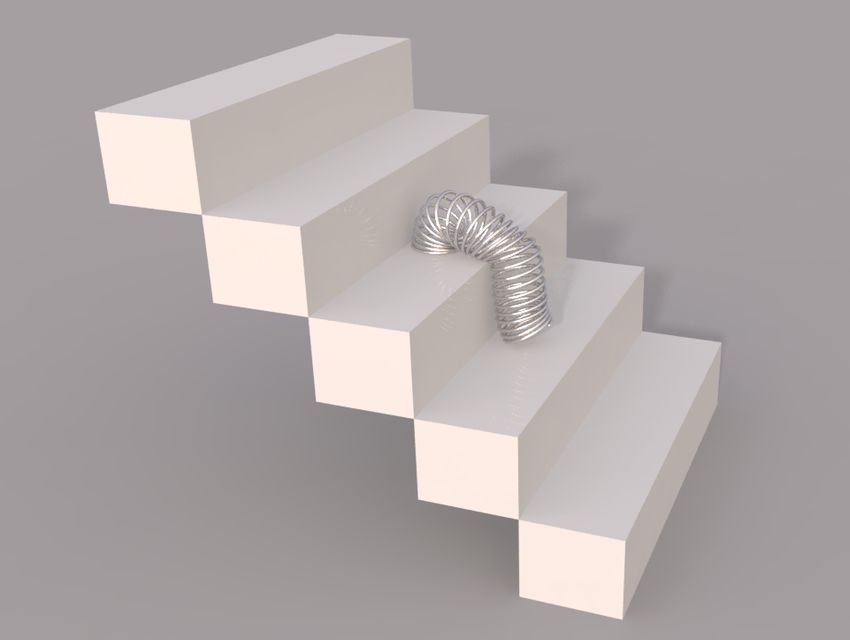
Deul et al. / Direct Position-Based Solver for Stiff Rods
with the help of ghost particles. This requires multiple constraints shearable and inextensible rods, i.e. Γ = 0. Therefore, we use a dis-
to keep the frame attached to the centerline. In a constraint graph, cretization of the rod which guarantees unshearability and enforces
where constraints and bodies are represented as nodes which are inextensibility with zero-stretch constraints (see Section 3.1).
connected by an edge if a constraint acts on a body (see [Bar96] for
The strain measure for bending and twisting is determined using
details), this setup leads to loops. Therefore, the method is not well
the Darboux vector Ω which is defined as
suited to be combined with a direct solver which often requires a
loop-free constraint graph. Recently, Deul et al. [DCB14] presented ∂
di (s) = Ω (s) × di (s). (2)
an approach to simulate rigid bodies with orientation constraints in ∂s
PBD. In our work we transfer their ideas to the discretization of This equation shows the close relationship between the Darboux
rods into rigid segments that are connected by our combined zero- vector Ω and the angular velocity ω of a rigid body. For ω the
stretch, bending and twisting constraint. Similar orientation con- same equation holds, except that the spatial derivative has to be
straints were used by Kugelstadt and Schömer [KS16] to simulate exchanged with the time derivative. Analogously to the angular ve-
Cosserat rods within PBD. Their constraints are modeled with a fi- locity the Darboux vector can be expressed in terms of the rotation
nite difference approximation of the strain measures from Cosserat quaternion
theory. We use a comparable formulation in our new combined ∂
stretch, bending and twisting constraint, which increases conver- Ω (s) = 2q̄(s)
q(s), (3)
∂s
gence and allows us to employ a direct solver.
where q̄ denotes the conjugate quaternion. In Equation (3) the Dar-
boux vector is expressed w.r.t. the material frame, which allows
3. Cosserat Model simple interpretations of its components. The first and second com-
ponent Ω 1 and Ω 2 measure local bending or curvature in d1 and d2
The Cosserat theory models a rod as a smooth curve r(s) : [s0 , s1 ] →
direction and the third component measures torsion around d3 . In
R3 , called centerline. To describe the bending and twisting degrees
the following we will allow rods with initial bending and torsion
of freedom, an orthonormal frame with basis {d1 (s), d2 (s), d3 (s)}
and we denote the rest pose Darboux vector as Ω 0 . We define the
is attached to each point of the centerline. In the following, the
strain measure of bending and torsion as
vectors di will be denoted as directors. The first and second di-
rector span the cross section of the rod, while the third director is ∂ ∂
Ω = Ω − Ω 0 = 2q̄
∆Ω q − 2q̄0 q0 , (4)
the cross section normal, as depicted in Figure 2. The directors can ∂s ∂s
which locally measures bending and torsion as the deviation of the
Darboux vector from the rest-pose Darboux vector. An important
property of the strain measure ∆Ω
Ω is that it is invariant to rigid
r(s) body motion.
d1
The continuous deformation energy can be defined as a quadratic
e3 d3 form of the strain measure. We define the bending and torsion en-
d2 ergy as
e2 EI1 0 0
1
Z
T
q(s) Eb = ∆ΩΩ K ∆Ω
Ωds, K= 0 EI2 0 , (5)
2
e1 0 0 GJ
Figure 2: Geometry of a continuous Cosserat rod. where K is a 3 × 3 matrix with material parameters for bending and
torsion stiffness, E is Young’s modulus and G is the torsion mod-
ulus of the material. In classical mechanics the shear modulus is
be parameterized with a rotation quaternion q(s), which computes used to define the stiffness with respect to torsion. However, since
the directors by rotating a frame that is initially parallel to the world in our work we aim for unshearable rods, we speak of the torsion
coordinate basis {e1 (s), e2 (s), e3 (s)}. The frame spanned by the di- modulus to emphasize that only torsion is affected by this param-
rectors of the initial rod configuration is called material frame. eter. The moments of inertia of the cross section I1 in direction d1
and I2 in direction d2 as well as the polar moment of inertia J are
Strain measures and deformation energies: The Cosserat theory given by:
defines the strain measure Γ that determines stretch and shear as Z Z
∂ I1 = x22 dx1 dx2 , I2 = x12 dx1 dx2 , J = I1 + I2 , (6)
Γ (s) = r(s) − d3 (s), (1) A A
∂s where A is the cross section area. In the special case of a circular
where r(s) is a unit-speed parametrization for the rod’s rest pose. cross section the inertia can be computed as I1 = I2 = 14 πr4 .
It follows that the tangent of centerline ∂s r has unit length and Γ
vanishes for the rest configuration because d3 also has unit length.
3.1. Discretization
Stretching or compression directly corresponds to length changes
of the centerline tangent, such that Γ measures stretch. Further- We aim for the simulation of inextensible and unshearable rods.
more, Γ measures how far the direction of the tangent and the direc- Therefore, we discretize the centerline as a chain of rigid segments
tor d3 deviate, which is denoted as shear. However, we aim for un- that are connected by a combination of zero-stretch, and bending
c 2018 The Author(s)
Computer Graphics Forum c 2018 The Eurographics Association and John Wiley & Sons Ltd.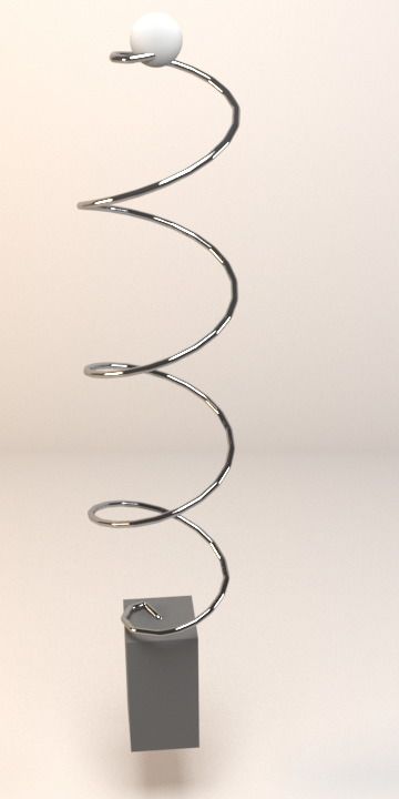
Deul et al. / Direct Position-Based Solver for Stiff Rods

                                                            Ωi                               tion (7)), which means the Jacobian of Ω i w.r.t. qi+1 is
                             Ω i−1                                                                    ∂        2
                                                                                                                                  < [qi ] 13×3 − [= [qi ]]× .

                qi−1                       qi                                                             Ωi =    −= [qi ]                                        (10)
                                                                         qi+1                       ∂qi+1      li
                                                                                             The derivative w.r.t. qi can be found analogously by using Ω i =
                                                                                             2                   2
                                                                                             li =[q̄i qi+1 ] = − li =[q̄i+1 qi ], which results in

Figure 3: The rod is discretized as a chain of rigid segments that                               ∂         2
                                                                                                                                < [qi+1 ] 13×3 − [= [qi+1 ]]× .

                                                                                                    Ω i = − −= [qi+1 ]                                            (11)
are connected by a combined zero-stretch, bending and twisting                                  ∂qi        li
constraint.

                                                                                             4. Constraint Solver
                                                                                             In this section we introduce an extension of the XPBD algorithm
and twisting constraints (see Figure 3). This guarantees that the                            proposed by Macklin et al. [MMC16] in order to simulate stiff
rod cannot be stretched. Furthermore, in contrast to methods us-                             Cosserat rods. We first give a brief overview of XPBD, then present
ing particles and a staggered constraint distribution, we solve the                          our extension of XPBD with a direct solver, and finally introduce
combined constraints between two segments simultaneously. As a                               our combined zero-stretch, bending and twisting constraint in de-
result, the convergence is increased and it is much easier to com-                           tail.
bine the constraints with a direct solver.
   We use the rigid segment orientations to discretize the direc-                            4.1. XPBD
tors, which also guarantees that the frames are aligned with the
centerline and shear deformation is not possible. Therefore, our                             Our constraint solver is based on the XPBD algorithm of Macklin
discretization of the rod automatically satisfies the hard constraint                        et al. [MMC16]. XPBD is an extension of Position-based dynamics
Γ = 0. Each rigid segment i is described by the position of its center                       which allows to apply physically meaningful material parameters
of mass pi and a rotation quaternion qi .                                                    by using compliance constraints. In this section we will summarize
                                                                                             the core ideas of XPBD and present the system of equations that
   In order to formulate a discrete bending and torsion energy,                              we have to solve.
we need to discretize the Darboux vector at constraint position i.
The derivative of the quaternion is discretized as finite difference                            The goal is to solve Newton’s equation of motion
approximation ∂s qi = l1i (qi+1 − qi ), where li denotes the average                                                     Mẍ = −∇U(x) + fext ,                    (12)
length of segment i and segment i + 1. Furthermore, we need to
                                                                                                                                                   T
evaluate the quaternion, which is only known at the center of the                            where M is the mass matrix, x = (x0 , x1 , ..., xn ) denotes the vec-
segments, at the segment position. Therefore, we interpolate the                             tor that collects all generalized coordinates of the physical system,
quaternion using the arithmetic mean of the adjacent quaternions                             U denotes the elastic potential and fext collects external forces like
as proposed by Spillmann and Teschner [ST07], such that the dis-                             gravity or wind forces. In our case x contains all mass centers and
crete Darboux vector becomes                                                                 quaternions and the block diagonal of M contains the masses and
                   1                                  2                                      inertia tensors of the rigid segments. Using an implicit Euler dis-
           Ωi =       = [(q̄i+1 + q̄i )(qi+1 − qi )] = = [q̄i qi+1 ] .               (7)     cretization yields:
                   li                                 li

Here we have to take the imaginary/vector part of the quaternion,                                    x(t + ∆t) − 2x(t) + x(t − ∆t)
                                                                                               M                                     = −∇U(x(t + ∆t)) + fext .
which is denoted as =[·]. This results in the discrete bending and                                                 ∆t 2
                                                                                                                                                              (13)
torsion energy
                                                                                             The elastic potential U(x) has the form
                                     1
                             Eb =         ΩTi Ki ∆Ω
                                                  Ωi .                               (8)                                  1
                                     2∑
                                         ∆Ω
                                       i
                                                                                                                    U(x) = C(x)T α −1 C(x),                       (14)
                                                                                                                          2

  In the following we will also need the Jacobian of the Darboux                             where C(x) = (C0 ,C1 , ...,Cm )T is a vector of constraint functions
vector. It can be computed by writing the quaternion product as                              and α is the diagonal compliance matrix describing the inverse
matrix-vector multiplication                                                                 stiffness. In case of the Cosserat bending and torsion potential we
                                                 !                                          identify C with ∆Ω  Ωi and α with K−1  i   which is defined by Equa-
                                 = [qi ]T                                                    tions (5) and (6). This means that the compliance matrix α de-

               < [qi ]                             < [qi+1 ]
  q̄i qi+1 =                                                  , (9)
              −= [qi ] < [qi ] 13×3 − [= [qi ]]×   = [qi+1 ]                                 scribes the material properties in terms of Young’s modulus, tor-
                                                                                             sion modulus and the cross section geometry. Taking the negative
where < [·] takes the real/scalar part of a quaternion, [·]× denotes                         gradient of the potential results in the elastic forces
the skew symmetric matrix, which can be used to write the cross                                             fel = −∇U(x) = −JT α −1 C = ∆t 2 JT λ ,               (15)
product as matrix-vector product and 13×3 is the 3 × 3 identity
matrix. The Darboux vector is the imaginary part of Equation (9)                             where J = ∇C denotes the constraint Jacobian. The elastic forces
scaled by the inverse of the average segment length (see Equa-                               are decomposed into direction and magnitude by introducing the

 c 2018 The Author(s)
Computer Graphics Forum c 2018 The Eurographics Association and John Wiley & Sons Ltd.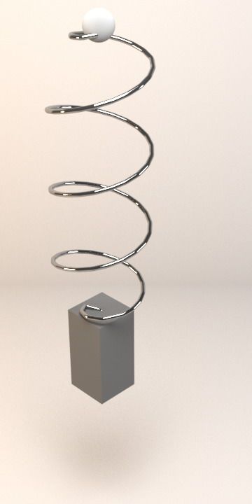
Deul et al. / Direct Position-Based Solver for Stiff Rods

                                                 α−1 C(x) with α̃
Lagrange multiplier λ = (λ0 , λ1 , ..., λm )T = −α̃            α=                      Gauss-Seidel solver is not well-suited for the simulation of stiff ob-
 α
∆t 2 . Plugging this into Equation (13)  yields                                        jects with many degrees of freedom like natural trees, because it
                                                                                       requires many iterations until it converges.
          M(x(t + ∆t) − x̃) − J(x(t + ∆t))T λ (t + ∆t) = 0,               (16)
                             C(x(t + ∆t)) + α̃
                                            αλ (t + ∆t) = 0,              (17)

where x̃ = 2x(t) − x(t − ∆t) + ∆t 2 M−1 fext . Note, that in contrast to
many other implicit integration methods, like for example the ones
of Hernandez et al. [HGCO11] or Aubry and Xian [AX15], Equa-                           4.2. Direct Solver
tion (16) contains an implicit constraint direction (ICD) J(x(t +
                                                                                       To overcome the problem of slow convergence, we solve the non-
∆t))T evaluated at the end of the time step. The inclusion of the
                                                                                       linear system for a rod and all its constraints with Newton’s method.
ICD helps in reducing jitter that occurs in high tension situations
                                                                                       We compute solutions to the linear KKT subproblems with a sparse
when enforcing length preserving constraints like our zero-stretch
                                                                                       direct solver. For general tree structures, the matrix in Equation (19)
constraints (see Goldenthal et al. [GHF∗ 07] for a detailed discus-
                                                                                       is not necessarily sparse. However, the problem can also be solved
sion). A different approach to avoid instabilities while enforcing
                                                                                       in linear time by considering Equation (18), which is always sparse
length preserving constraints is to introduce a geometric stiffness
                                                                                       for trees. This system of equations can be solved by a modified ver-
term to the system matrix (see Tournier et al. [TNGF15]). How-
                                                                                       sion of Baraff’s linear-time solver [Bar96], where the compliance
ever, our method is based on an algorithm which already employs
                                                                                       factors must be considered. To simplify the notation we multiply
an ICD. As such, using the geometric stiffness term is not devel-
                                                                                       the second row in Equation (18) with −1, denote the matrix as H
oped further in our paper.
                                                                                                             λi = −b, yielding
                                                                                       and define C(xi ) + α̃λ
   The system of equations (16) and (17) is in general non-linear
and can be solved with Newton iterations. Macklin et al. [MMC16]
                                                                                                               −JT

                                                                                                       M                   ∆x       ∆x    0
linearize these equations and propose several simplifications, re-                                                              =H     =    .                             (22)
                                                                                                       −J      −α̃
                                                                                                                α           λ
                                                                                                                           ∆λ        λ
                                                                                                                                    ∆λ   −b
sulting in the following KKT system for the i-th iteration:
                     −J(xi )T

             M                   ∆x                   0
                                        =  −                    ,    (18)              This system equals the notation in [Bar96] with compliance α̃         α
            J(xi )       α
                         α̃      ∆λ λ                    αλ i
                                                C(xi ) + α̃                            added in the lower right submatrix of matrix H. It can be solved in
                               T                                                     linear time by reordering the equations as described in [Bar96]. The
where the vector ∆xT , ∆λ    λT     is the root update of the Newton                   reordering can be done once during initialization because it remains
                           T                 T                T
                                                                                       constant as long as the constraint topology does not change. After

step (xi+1 )T , (λ λi+1 )T               λi )T + ∆xT , ∆λ
                             = (xi )T , (λ                    λT . The
                                                                                       that the system can be solved using a sparse LDLT decomposition.
number of equations in (18) can be reduced by applying the Schur                       In typical scenarios of computer graphics simulated objects often
complement, which results in                                                           interact with each other by collisions. However, a rod that collides
              h                    i
               J(xi )MJ(xi )T + α̃
                                 α ∆λ λ = −C(xi ) − α̃λ  λi .        (19)              at two points with the environment forms a loop. Furthermore, a rod
                                                                                       representing a rope, e.g. a clothes line, is usually fixed at both ends
The updates of the positions are determined by                                         to the environment and therefore also forms a loop. But, our direct
                                                                                       solver only supports acyclic structures and no loops. Therefore, we
                         ∆x = M−1 J(xi )∆λ.                               (20)
                                                                                       alternate the computation of our rod solver with the computations
                                                                                       of the non-linear Gauss-Seidel solver for loop-closing constraints
   Macklin et al. solve Equation (19) with a non-linear Gauss-
                                                                                       and collision constraints. Thus, the position corrections of the direct
Seidel solver. This solver iterates over all constraints and computes
                                                                                       solver and the position corrections due to collisions or loop closing
solutions for each constraint in isolation. Hereby, the solution ∆λ j
                                                                                       constraints are transferred immediately from the one solver to the
to a single constraint equation with index j is computed as
                                                                                       other. Algorithm 1 presents the alternation of direct solver and non-
                               −C j (xi ) − α̃ j λij                                   linear Gauss-Seidel solver, which from now on will be called KK-
                    ∆λ j =                              .                 (21)         T/GS solver, in the context of the XPBD time step. At the beginning
                             ∇C j M−1 ∇CTj + α̃ j
                                                                                       of the time step the unconstrained positions are predicted by inte-
Immediately, after computing ∆λ j position updates ∆x are com-                         grating the velocities and external forces (lines 1 and 2). Next, the
puted using Equation (20) and applied to the positions xi . As such,                   initial values of the KKT/GS method are defined. Beginning from
the non-linear system in Equation (19) is never build completely.                      line 5 the rod, collision, or loop-closing constraints are solved iter-
It follows, that at no point in time there exists a subproblem in                      atively. The iterations are stopped if the residual maximal error in
the sense of Newton’s method. To sum up, the non-linear Gauss-                         the constraint functions is smaller than a predefined threshold η. In
Seidel solver computes individual Newton problems per constraint                       each iteration, first the KKT subproblems for the simulation of the
and the solutions of the constraints influence each other through the                  rods are solved using our linear-time solver and the positions of the
immediately updated positions. For infinitely stiff constraints with                   corresponding rigid segments as well as the Lagrange multipliers λ
α̃ j = 0, Equation (21) reduces to the Lagrange multiplier formula                     are updated (lines 6 to 9). Then, the collision and loop closing con-
of standard Position-based dynamics [MHHR07]. This shows, that                         straints are solved successively in non-linear Gauss-Seidel fashion
XPBD is a generalization of PBD that allows for using physically                       (lines 10 to 14). After the solver iterations are finished the position
meaningful material stiffness parameters. However, the non-linear                      at the end of the time step is set and the velocity is updated.

                                                                                                                                                           c 2018 The Author(s)
                                                                                          Computer Graphics Forum c 2018 The Eurographics Association and John Wiley & Sons Ltd.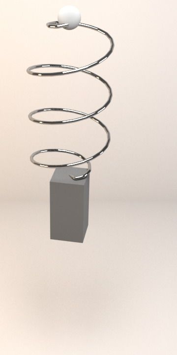
Deul et al. / Direct Position-Based Solver for Stiff Rods
Algorithm 1 Time Step with
1: for all rigid segments do −= [q]T
1
2: x̃ ← x(t) + ∆tv(t) + ∆t 2 M−1 fext G(q) =
2 < [q] 13×3 + [= [q]]×
, (27)
0
3: x ← x̃
0
4: λ ← 0 where G(q) describes the relationship between the quaternion ve-
5: while C(xi ) + α̃ αλ i > η do locity q̇ and the angular velocity ω as q̇ = G(q)ω and can also be
∞ used on the orientation level.
6: for all rods do
7: solve Equation (22) using our linear-time solver The mass matrix of each segment is given by
8: update xi+1 ← xi + ∆x
m13×3 0
i+1 i
9: update λ ← λ + ∆λ λ ρli I1 0 0
10: for all collision or loop-closing constraints do M= , (28)
0 0 ρli I2 0
11: compute ∆λ with Equation (21) 0 0 ρli J
12: compute ∆x with Equation (20)
13: update xi+1 ← xi + ∆x where li is the length of segment i, ρ denotes the mass density, m is
i+1 i the mass of the segment and the moments of inertia I1 , I2 and J are
14: update λ ← λ + ∆λ λ
given by Equation (6). In our examples, we assume an isotropic rod
15: i ← i+1 with circular cross-section. As such, we approximate the geometry
16: x(t + ∆t) ← xi of a single segment with a cylinder and set the values for m, I1 , I2
1
17: v(t + ∆t) ← ∆t (x(t + ∆t) − x(t)) and J accordingly.
5. Results
4.3. Rod Constraint
We tested the performance of our method in various experiments.
In the following we define the constraint functions and their Jaco- All experiments in this section were performed on a single core of
bians for the zero-stretch, bending and twisting constraints, which an Intel Core i7-2600, 8GB of memory.
we use to simulate elastic rods.
We combine the zero-stretch, bending and twisting constraints Cantilever beam: To validate our approach we fixed a rod of
that couple two rigid segments into one six-dimensional constraint length 10m and a radius of 0.5m at one end. At the other end
with the constraint function we applied a force F of 1000N. The rod is discretized into 50
! segments and has a Young’s modulus E of 1GPa. In the follow-
R(q1 )p1 +h x1 − R(q2 )pi2 − x2 ing we compare the deflection δC at the
C(x1 , q1 , x2 , q2 ) = 2 0 0 . (23) end of the rod with the
li = q̄1 q2 − q̄1 q2 analytical solution computed as δC = FL3 / (3EI), where I is
The first three rows connect a point p1 on segment 1 with a point the moment of the cross section (see Equation (6)). The simu-
p2 on segment 2. These points are given in the local coordinates lated deflection is 6.7949 · 10−3 m whereas the analytical solution
of the corresponding segment and are transformed to world coor- is 6.7906 · 10−3 m. As a result, we have a deviation of only about
dinates by applying the rotation matrix R(q) and translation x of 4.3 · 10−6 m. For small deformations the elastic potential is nearly
their segment. The last three rows constrain bending and twisting linear, which means that this result could be reached after one KK-
(see Section 3.1). The stiffness of each constraint is given by a 6 ×6 T/GS iteration as expected.
compliance matrix
Wilberforce pendulum: We underpin the physical plausibility of
1 σ −1
0 our approach with the simulation of a Wilberforce pendulum (see
α̃ = 2
α . (24)
∆t 0 K−1 Figure 4). The pendulum consists of a helical spring that is fixed at
its upper end. A mass is attached to the lower end. At the beginning
The diagonal matrix σ is the zero-stretch stiffness matrix. Further-
of the experiment the mass is moved out of the resting position.
more, the bending and torsion stiffness K is the same as in Equa-
The accompanying video as well as Figure 5 show that the mass al-
tion (5). Due to stability considerations of the solver and to avoid
ternates between translational and rotational movement. This phe-
bad conditioning of the system matrix we weaken the inextensibil-
nomenon is the result of coupled oscillations which are faithfully
ity of the zero-stretch constraint slightly by setting the diagonal of
reproduced by our approach.
σ −1 to values between 10−8 and 10−10 in our simulations.
Further, we need the constraint Jacobians w.r.t. segment 1 and Slinky: We simulated a Slinky walking down a stairway (see Fig-
segment 2, which are defined by ure 1). Using this scenario we tested the performance of the rod
solver in presence of a high number of self-collisions and colli-
13×3 − [R(q1 )p1 ]×
!
∂C ∂C sions with the environment. The Slinky consists of 500 rigid seg-
J1 = , G(q1 ) = Ω
∂Ω (25)
∂x1 ∂q1 0 ∂q1
G(q1 ) ments and was simulated with a time step size of 10ms at three
−13×3 [R(q2 )p2 ]× iterations of the alternating KKT solver for rods and non-linear
!
∂C ∂C
J2 = , G(q2 ) = Ω
∂Ω (26) Gauss-Seidel approach for collisions (see Section 4.2). We used
∂x2 ∂q2 0 G(q2 )
∂q 2 an approach based on signed distance fields [KDB16] for collision
c 2018 The Author(s)
Computer Graphics Forum c 2018 The Eurographics Association and John Wiley & Sons Ltd.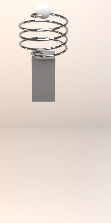
Deul et al. / Direct Position-Based Solver for Stiff Rods
Figure 4: First image: At the beginning of the simulation the pen-
dulum bob of the Wilberforce pendulum is raised and then falls
down. Second image: The bob moves up and down and begins to
rotate around the vertical axis. Third image: After the first 12 sec-
onds the translational up and down movement of the bob changes
almost entirely to a rotation around the vertical axis. Fourth im-
age: After about another 12 seconds the rotational movement has Figure 6: An elastic rod under torsion shows the formation of plec-
completely disappeared and the bob moves only upward and down- tonemes.
ward.
4
Translation z (in meters)
Rotation θ (in radians)
2
0
−2
−4
0 10 20 30 40
Time (sec)
Figure 5: Translation z and rotation θ of the pendulum bob as a
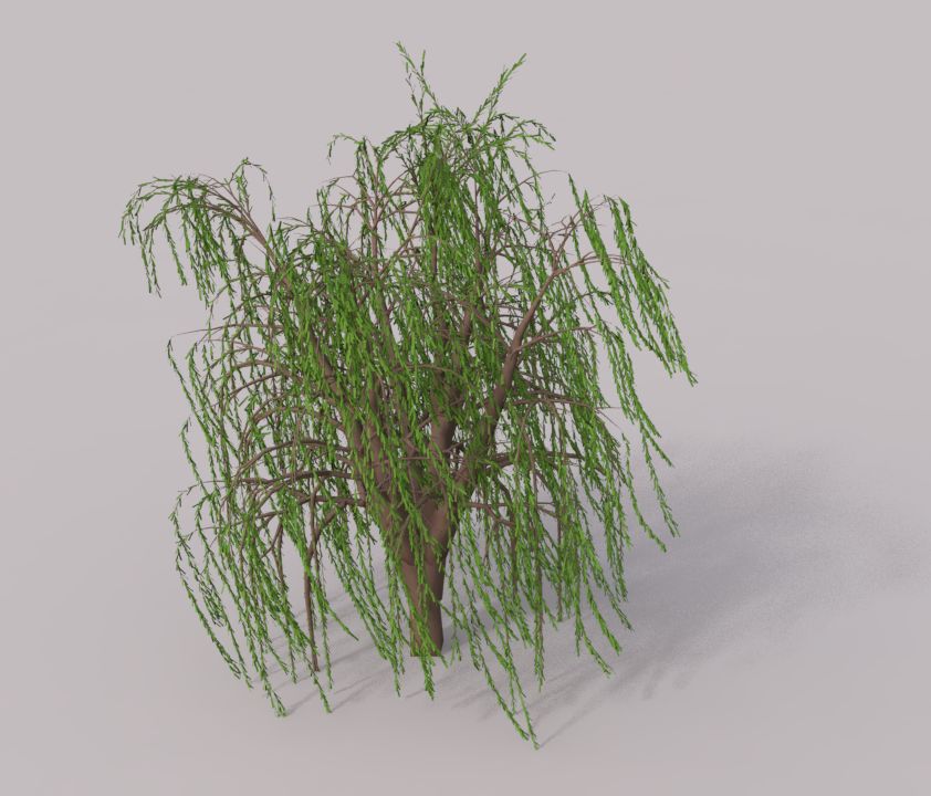
function of time for our Wilberforce pendulum experiment. Figure 7: The weeping willow model represents a tree with thick,
as well as long, slender branches with many segments.
detection. The result of the simulation is shown in Figure 1 and the Tree simulation: The simulation of natural trees is one of the
accompanying video. The Slinky descends five stairs before stop- most demanding applications of rod simulation. Many approaches
ping at the floor, while the solver handles hundreds of collisions per [BWR∗ 08, Ber09, HKW09, ZB13, AX15] applied some kind of rod
time step. or beam model to tree simulation. In this paragraph we show how
our approach performs in this complex simulation task. Our rod
Knot: To demonstrate that our method is not only applicable to model was tested with three tree models with different topology,
stiff rods, but to soft elastic rods as well, we simulated a strand un- which were generated with Blender 2.78a’s sapling tree generator.
der torsion. The rod is fixed at both ends. During the simulation, A white birch represents a typical deciduous tree (see Figure 1).
the left fixture is translated towards the right, while it performs ten The second tree is a weeping willow (see Figure 7) with long slen-
full rotations. Figure 6 and the accompanying video show the ex- der branches. Conifers with many small leaves are represented by
pected formation of plectonemes. These confirm the soundness of a pine model (see Figure 8). Besides the trunk and the branches,
our material model and show that self-collisions are handled well. we also represent each leaf of the tree with a single rigid segment
c 2018 The Author(s)
Computer Graphics Forum c 2018 The Eurographics Association and John Wiley & Sons Ltd.Deul et al. / Direct Position-Based Solver for Stiff Rods
There is no need for tuning parameters for each branch by hand and
simulations naturally show plausible behavior.
Comparison of the KKT/GS solver to the non-linear Gauss-
Seidel solver: We compared the performance of the KKT/GS
solver to the solution computed with the non-linear Gauss-Seidel
solver of Macklin et al. [MMC16] in two scenes. In the first scene
we tested the cantilever beam example from above with differ-
ent discretizations. We ran the simulation for 60s to let the beam
swing out of the initial state and come to rest. This part of the
the simulation was performed using our direct solver at three it-
erations per time step. Thereafter, we ran 500000 KKT/GS itera-
tions as well as 500000 non-linear Gauss-Seidel iterations (one GS
iteration means one traversal through the whole matrix) and mon-
itored the Chebyshev norm of the residual error in b (see Equa-
tion (22)). The results are depicted in Figure 9. After one iteration
the error of the KKT/GS solver is about 2.2 · 10−13 , 2.8 · 10−16 ,
and 4.4 · 10−18 , and the error of the non-linear Gauss-Seidel solver
is 10−1 , 5 · 10−3 , and 3.5 · 10−4 for a discretization of 1000, 50,
and 8 segments, respectively. In the first three iterations the error
of the KKT/GS solver decreases even further to about 4.4 · 10−16 ,
9.4 · 10−19 , and 5.9 · 10−19 . However, the non-linear Gauss-Seidel
solver needs about 1000 and 50000 iterations for the beams with
8 and 50 segments, respectively, to arrive at an error value which
Figure 8: An example for conifers, which contain a huge number
is comparable to the error after only one KKT/GS iteration. The
of small leaves, is given by this pine model.
smallest error for the non-linear Gauss-Seidel solver with a 1000
segment beam is about 1.3 · 10−4 after 500000 iterations. How-
Model Segments Avg. pos. corr. time ever, the direct solver used to compute the KKT subproblems in-
Birch 29973 658.08ms creases the computational cost of one KKT/GS iteration compared
Willow 38825 870.31ms to one non-linear Gauss-Seidel iteration. In the case of the can-
Pine 49548 1048.74ms tilever beam, one iteration of the KKT/GS solver is 3.1 times more
costly than one iteration of the non-linear Gauss-Seidel solver. To
Table 1: Number of segments and average time required for the find out if the improved convergence is worth the increased cost,
position correction in the respective tree simulations. we compare the error after one KKT/GS step with the error af-
ter four Gauss-Seidel iterations. While the Gauss-Seidel solver still
has an error of 1.4 · 10−3 , the error of our KKT/GS solver remains
at merely 2.8 · 10−16 . It follows that the increased convergence of
connected with the combined zero-stretch, bending and twisting the KKT/GS solver outweighs the computational overhead by far.
constraint to the tree. As such, our model can capture the subtle
The second test scene is the birch simulated in an increasing
movement of leaves in the wind. Wind is modeled by a procedural
wind field. We simulated the scene in several runs. For each suc-
wind field. We first start with a subtle wind force which is succes-
cessive run we decreased the threshold for the Chebyshev norm of
sively increased to stormy conditions. Then we stop the wind to
the residual error in b. Note, that the stiffness of the simulated ob-
show that the model comes to rest. Each tree was simulated with
ject decreases if the residual error in b is too large. Thus, a threshold
a large time step size of 40ms and three iterations per time step to
that is too high will result in a perceptually wrong animation. Our
guarantee a upper bound for the residual error of 10−6 . The tree
own experiments have shown that an error threshold of η = 10−6
models consist of 29973, 38825, and 49548 rigid segments for the
is sufficient to reach a relative change in stiffness of about 3%. The
birch, the willow, and the pine, respectively. The Young’s modulus
best threshold value would be 10−9 after which the measured de-
is set to 12.5GPa and the torsion modulus to 6.5GPa for the trunk
viation in stiffness does not change significantly. Table 2 shows the
and the branches. For the leaves, which are more flexible, we chose
required KKT/GS iterations and non-linear Gauss-Seidel iterations
a Young’s modulus of 1.2GPa and a torsion modulus of 0.6GPa.
at different threshold values. The iteration count of the KKT/GS
The density was set to 1000kg/m3 . Our results show a convincing
solver stays in a range of 1 to 5 iterations. The Gauss-Seidel solver
movement of the tree geometry in the wind. Furthermore, the sim-
on the other hand requires more than 200 iterations even for a
ulation stays stable even under large wind forces. The average time
threshold of 10−2 . Though, at this threshold the residual errors lead
taken by the position correction for the tree simulations is given in
to a significant deviation of the simulation to the expected result.
Table 1. Besides the fast simulation, a big advantage of our model
compared to previous rod simulation approaches for Position-based For this scene one iteration of the KKT/GS solver is 5.6 times
dynamics is that we can use physically meaningful material param- more costly than one iteration of the non-linear Gauss-Seidel
eters. The thickness of a branch automatically changes its stiffness. solver. This factor is higher than for the cantilever beam due to the
c 2018 The Author(s)
Computer Graphics Forum c 2018 The Eurographics Association and John Wiley & Sons Ltd.Deul et al. / Direct Position-Based Solver for Stiff Rods
100 Average iterations Pos. corr.
Error threshold η KKT/GS Gauss-Seidel speedup
10−2 1.49 208.73 25.5
10−5 10−6 2.98 2055.23 124.8
10−9 4.15 3629.69 164.6
GS1000 KKT1000
Table 2: Even for large error thresholds our KKT/GS solver needs
|b|∞
−10 GS50 KKT50
10 significantly fewer iterations than the Gauss-Seidel solver. Not only
GS8 KKT8
does this compensate for the cost of the KKT/GS iterations, but it
also speeds up the position correction by multiple orders of magni-
10−15 tude. Measurements are taken from the birch example.
10−20
100 101 102 103 104 105 106 Comparison to previous methods: We compared our method to
Iteration Position-based Elastic Rods (PBER) by Umetani et al. [USS14]
and Position and Orientation Based Cosserat Rods (PaOBCR) by
Kugelstadt and Schömer [KS16]. In order to make the comparison
Figure 9: Convergence of the Gauss-Seidel solver (GS) and as fair as possible, we exchanged the PBD-stiffness parameter of
KKT/GS (KKT) solver in the cantilever beam scene, plotted on a both approaches with a compliant implementation for bending and
log-log scale. Measurements are shown for discretizations of the twisting. Furthermore, we lumped the segment masses of our model
beam with 1000, 50, and 8 segments. to the particle masses of these approaches. In case of the approach
of Kugelstadt and Schömer we applied the part of the inertia tensor
of our segments which corresponds to a rotation around the axis
orthogonal to the rod centerline to their quaternion weighting wq .
However, the approach of Umetani et al. describes no direct rep-
10−3 resentation of inertia. Inertia is indirectly modeled by the weight
distribution between particles and ghost particles. We distributed
the lumped segment mass evenly between the two particles and
10−7 PBER one ghost particle representing a segment of the rod. For the fol-
PaOBCR lowing comparison we solved all constraints of the three different
|b|∞
GS approaches with the non-linear Gauss-Seidel solver, even our own
10−11 KKT combined zero-stretch, bending and twisting constraint, to present
convergence properties and mathematical effort. Furthermore, we
compared these results to the performance of our KKT/GS solver
10−15 approach. For this test we also employed the cantilever beam with
50 segments. As shown in Figure 10 PBER and PaOBCR con-
verge slower than our combined zero-stretch, bending and twisting
10−19 constraint. However, our combined constraint solved with the non-
100 101 102 103 104 105 106 linear Gauss-Seidel solver is 13.9 times computationally more ex-
Iteration pensive than its cheapest competitor, PaOBCR. Even after compar-
ing the cost of both methods after they reach the same error thresh-
old PaOBCR ist cheaper. However, PaOBCR would loose its essen-
Figure 10: Convergence of different simulation methods for the tial advantage of avoiding matrix inversions in a combination with a
cantilever beam discretized with 50 segments, plotted on a log-log direct solver in a KKT/GS method. Furthermore, it is not clear how
scale. The methods in comparison are Position-Based Elastic Rods to combine the staggered distribution of kinematic values like posi-
(PBER), Position and Orientation Based Cosserat Rods (PaOBCR), tion and orientation of the PaOBCR model with a direct solver for
the Gauss-Seidel (GS) solver and our KKT/GS (KKT) solver. trees. Even though, PaOBCR is faster than our combined constraint
solved with non-linear Gauss-Seidel, the KKT/GS method with our
direct solver is by far the fastest approach. PaOBCR needs over
100000 iterations to decrease the order of magnitude in the residual
error to a value that is reached by the KKT/GS method after only
increased complexity of the birch. The branching of the tree results one iteration. Thereby PaOBCR is about 5890 times more expen-
in an increase of matrix-matrix products in our direct solver. De- sive. Another advantage of our direct solver is that all constraints
spite the even higher costs per iteration compared to the cantilever are solved at once, which means that instabilities arising from cer-
scene, the increased convergence leads to a speedup of two orders tain constraint orderings as reported by Umetani et al. [USS14] and
of magnitude for the birch scene (see Table 2 for the exact values). Kugelstadt and Schömer [KS16] are completely avoided.
c 2018 The Author(s)
Computer Graphics Forum c 2018 The Eurographics Association and John Wiley & Sons Ltd.Deul et al. / Direct Position-Based Solver for Stiff Rods
6. Conclusion [BAV∗ 10] B ERGOU M., AUDOLY B., VOUGA E., WARDETZKY M.,
G RINSPUN E.: Discrete viscous threads. ACM Transactions on Graphics
We presented a KKT/GS approach for the efficient simulation 29, 4 (2010), 116. 3
of stiff, inextensible elastic rods in the Position-based dynamics [Ber09] B ERTAILS F.: Linear time super-helices. Computer Graphics
framework. It allows the simulation of hard constrains and elas- Forum 28, 2 (2009), 417–426. 3, 8
tic potentials with physically meaningful material parameters in [BET14] B ENDER J., E RLEBEN K., T RINKLE J.: Interactive Simulation
a unified framework. Even though the solution of our KKT sub- of Rigid Body Dynamics in Computer Graphics. Computer Graphics
problems has higher computational costs than one iteration of non- Forum 33, 1 (2014), 246–270. 2
linear Gauss-Seidel, this is outweighed by the huge increase in [BMM14] B ENDER J., M ÜLLER M., M ACKLIN M.: A Survey on
convergence, so that large and stiff objects can be simulated with Position-Based Simulation Methods in Computer Graphics. Computer
a speedup of two orders of magnitude. By using XPBD and the Graphics Forum 33, 6 (2014), 228–251. 2, 3
KKT/GS solver, our method does not have the major drawbacks [BPGK06] B OTSCH M., PAULY M., G ROSS M. H., KOBBELT L.:
of PBD, namely that the material stiffness does not depend on the Primo: coupled prisms for intuitive surface modeling. In Symposium
number of iterations, the time step and the ordering of the con- on Geometry Processing (2006), no. EPFL-CONF-149310, pp. 11–20. 3
straints. [BW98] BARAFF D., W ITKIN A.: Large steps in cloth simulation. In
International Conference on Computer Graphics and Interactive Tech-
Our main drawback compared to some other methods in rod or niques (1998), ACM, pp. 43–54. 2
tree simulation is that we often have to solve more than one system [BWR∗ 08] B ERGOU M., WARDETZKY M., ROBINSON S., AUDOLY
of linear equations per time step. This is a result of the particu- B., G RINSPUN E.: Discrete elastic rods. ACM Trans. Graph. 27, 3
lar time discretization of XPBD which, however, leads to increased (2008), 1–12. 3, 8
stability. Furthermore, we chose XPBD intentionally to achieve a [CCK05] C HOE B., C HOI M. G., KO H.-S.: Simulating complex hair
tight coupling of our rod simulations with the vast amount of solu- with robust collision handling. In ACM SIGGRAPH / Eurographics Sym-
tions for different physical effects that have been published for the posium on Computer Animation (2005), ACM, pp. 153–160. 2
Position-based dynamics framework. In order to reduce the compu- [DCB14] D EUL C., C HARRIER P., B ENDER J.: Position-based rigid-
tational effort, we want to work on improving the performance of body dynamics. Computer Animation and Virtual Worlds (2014). 4
our direct solver. One of the most time consuming parts is the fac- [GHF∗ 07] G OLDENTHAL R., H ARMON D., FATTAL R., B ERCOVIER
torization of the system matrix. We want to develop an optimized M., G RINSPUN E.: Efficient simulation of inextensible cloth. ACM
solver in the future. Transactions on Graphics 26, 3 (2007). 2, 6
[GS07] G RÉGOIRE M., S CHÖMER E.: Interactive simulation of one-
A minor limitation of our approach is that XPBD makes some dimensional flexible parts. Computer-Aided Design 39, 8 (2007), 694–
simplifications in formulating the system for the KKT subprob- 707. 3
lems. Nevertheless, our method is numerically stable and delivers [Had06] H ADAP S.: Oriented strands: dynamics of stiff multi-body sys-
plausible results, like our comparison to the analytical solution has tem. In ACM SIGGRAPH / Eurographics Symposium on Computer Ani-
shown. In many interactive applications, like games, these features mation (2006), Eurographics Association, pp. 91–100. 3
are more important than the highest physical accuracy. For the fu- [HGCO11] H ERNÁNDEZ F., G ARRE C., C ASILLAS R., OTADUY
ture we plan to investigate if we can modify our method, so that it M. A.: Linear-time dynamics of characters with stiff joints. In Proceed-
works without the simplifications made in XPBD. ings of V Ibero-American Symposium on Computer Graphics (2011). 2,
6
[HH13] H AN D., H ARADA T.: Tridiagonal matrix formulation for inex-
Acknowledgment tensible hair strand simulation. In Proceedings of Virtual Reality Inter-
actions and Physical Simulations (VRIPhys) (2013), The Eurographics
This work is supported by the German Research Foundation (DFG) Association. 2
under contract numbers BE 5132/3-1 and GSC 233/2, and by the [HKW09] H ABEL R., K USTERNIG A., W IMMER M.: Physically guided
’Excellence Initiative’ of the German Federal and State Govern- animation of trees. Computer Graphics Forum 28, 2 (2009), 523–532. 8
ments and the Graduate School of Computational Engineering at [IMP∗ 13] I BEN H., M EYER M., P ETROVIC L., S OARES O., A NDER -
TU Darmstadt. SON J., W ITKIN A.: Artistic simulation of curly hair. In ACM SIG-
GRAPH / Eurographics Symposium on Computer Animation (2013),
ACM, pp. 63–71. 2
References [KDB16] KOSCHIER D., D EUL C., B ENDER J.: Hierarchical hp-
adaptive signed distance fields. In ACM SIGGRAPH / Eurographics
[Ant05] A NTMAN S.: Nonlinear Problems of Elasticity; 2nd ed. Symposium on Computer Animation (2016), Eurographics Association.
Springer, Dordrecht, 2005. 3 7
[AX15] AUBRY J.-M., X IAN X.: Fast implicit simulation of flexi- [KS16] K UGELSTADT T., S CHÖMER E.: Position and orientation based
ble trees. In Mathematical Progress in Expressive Image Synthesis II. Cosserat rods. In ACM SIGGRAPH / Eurographics Symposium on Com-
Springer, 2015, pp. 47–61. 2, 6, 8 puter Animation (2016), Eurographics Association, pp. 169–178. 4, 10
[BAC∗ 06] B ERTAILS F., AUDOLY B., C ANI M.-P., Q UERLEUX B., [LL09] L ANG H., L INN J.: Lagrangian field theory in space-time for
L EROY F., L ÉVÊQUE J.-L.: Super-helices for predicting the dynamics geometrically exact Cosserat rods. ITWM, Fraunhofer Inst. Techno-und
of natural hair. ACM Trans. Graph. 25, 3 (2006), 1180–1187. 3 Wirtschaftsmathematik, 2009. 3
[Bar96] BARAFF D.: Linear-time dynamics using Lagrange multipli- [LLA11] L ANG H., L INN J., A RNOLD M.: Multi-body dynamics simu-
ers. In International Conference on Computer Graphics and Interactive lation of geometrically exact Cosserat rods. Multibody System Dynamics
Techniques (1996), ACM, pp. 137–146. 2, 4, 6 25, 3 (2011), 285–312. 3
c 2018 The Author(s)
Computer Graphics Forum c 2018 The Eurographics Association and John Wiley & Sons Ltd.You can also read