Interbank Contagion Risk in China Under an ABM Approach for Network Formation
←
→
Page content transcription
If your browser does not render page correctly, please read the page content below
Interbank Contagion Risk in China Under an
       ABM Approach for Network Formation
                          Shiqiang Lin∗, Hairui Zhang†
                                      Jan 2021

                                       Abstract
          There are growing studies on the contagion risk of the Chinese inter-
      bank market. However, many of these studies are based on the maximum
      entropy method to estimate China’s interbank network. Such a method
      has been criticized as unrealistic because it underestimates contagion risk
      by producing too many links (Mistrulli, 2011; Upper, 2011). This paper
      uses an agent-based model (ABM) to construct an interbank network for
      the Chinese interbank market. Our data contain 299 commercial banks
      with financial data from 2014 to 2019. The simulation result of credit
      shocks indicates that rural commercial banks and foreign banks are less
      resilient to shocks. One of the reasons why banks are prone to failure is the
      excessiveness of interbank lending, which makes suggestion to policymak-
      ers to consider introducing some controls over banks’ interbank lending
      size compared to their equity bases.
          Keywords: interbank network, contagion risk, agent-based modeling,
      Chinese banking sector

1     Introduction
The global interbank market’s systemic risk has been a growing concern since
the financial crisis in 2008. When an idiosyncratic shock to one bank or a group
of banks is transmitted to other banks and economic sectors, it triggers default
risks among financial institutions all over the world (Hasman, 2012). The effect
of an internal or external idiosyncratic shock to the interbank market is called
contagion, which has been studied by many researchers (c.f. Brownless, Hans
and Nualart, 2014; Acemolu, Ozaglar, and Salihi, 2015). However, one of the
main constraints of studying the interbank contagion risk is the lack of empiri-
cal data on the interbank claims. The reason is that interbank transactions are
arranged over the counter. Therefore the data are usually not publicly available
   ∗ Faculty of Business and Economic, University of Antwerp, Antwerpen, Belgium, corre-

spondence email: lin.andrew@foxmail.com
   † Faculty of Business and Economic, University of Antwerp, Antwerpen, Belgium

                                           1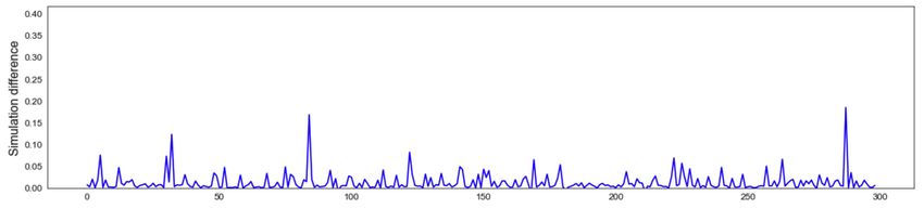
in many countries. Alternatively, academia relies on methods such as maxi-
mum entropy (ME) (c.f. Upper and Worms, 2004; Boss, Elsinger, Summer and
Thurner, 2004; Wells, 2004; Mistrulli, 2011) and minimum density (MD) (c.f.
Anand, Craig, and Von Peter, 2014) to estimate the interbank network struc-
tures. These methods are based on interbank assets and interbank liabilities
from the bank’s balance sheet, using a standard iterative algorithm to fill in the
blank for the bilateral liabilities of the interbank liabilities matrix. However, the
findings from Anand et al. (2014) conclude that when used in a stress test, ME
(MD) tends to underestimate (overestimate) contagion. Anand et al. (2014)
inspire Liu, Paddrik, Yang, and Zhang (2020) to develop an agent-based model
(ABM) as an alternative to ME and MD. Using their ABM approach, Liu et al.
(2020) reconstruct interbank networks based on 6600 US banks’ decision rules
and behaviors between 2001 and 2014. Their model produces a network struc-
ture that is well-bounded by the established ME and MD methods, as Anand
et al. (2014) find that the actual network lies between that for ME and MD.
    As the world’s second-largest economy, the Chinese banking industry has
surpassed that of the European Union in size, and the world’s four largest
banks in 2018 are Chinese banks (Deloitte, 2019). Despite the size of the Chi-
nese banking sector, fewer studies on the Chinese interbank market have been
published than those on the European and US markets. Furthermore, those
studies mainly focus on ME (Xie, Liu, Wang, and Xu, 2016; Cao, Li, Chen, and
Chen, 2017; Sun, 2020). Suppose that the findings of Anand et al. (2014) and
Liu et al. (2020) on ME holds. It implies that previous studies on the Chinese
interbank market introduces a substantial downward bias on risk estimation.
    Furthermore, most studies focus on the contagion effect for Tier-1 banks (6
state-owned banks) and Tier-2 banks (12 joint-stock banks) (cf. Xie et al., 2016;
Cao et al., 2017). Less attention has been paid to lower-tiered banks, such as
city commercial banks and rural commercial banks (Sun, 2020). Nevertheless,
lower-tiered banks are more vulnerable to contagion risks and are essential to
local economies and small-and-medium enterprises (SMEs). Thus they should
also be included in the analysis to understand more comprehensively the Chinese
interbank market. Thus, we include Tier 1, Tier 2, and lower-tiered banks in
our study.
    We focus on the following research questions. Firstly, how are the Chinese
interbank network topologies under the ABM method compared to those under
ME and MD? Secondly, what are the contagions of credit shocks on the Chinese
interbank network? Thirdly, do the shocks’ effects on lower-tiered banks (below
Tier 2) differ from those on higher-tiered banks (Tier 1 and 2)? If so, how
different?
    We contribute to the literature in the following aspects. Firstly, unlike pre-
vious researches using ME to study the interbank network in China that un-
derestimates the contagion risk, we use an ABM approach. Secondly, an ABM
approach bears the rationale that each bank acts as an agent to achieve its
lending and borrowing target ratios. Under ABM, the interbank network is en-
dogenously formed by simulating heterogeneous agents following some decision
rules. As Battiston and Martinez-Jaramillo (2018) point out, the endogenous

                                         2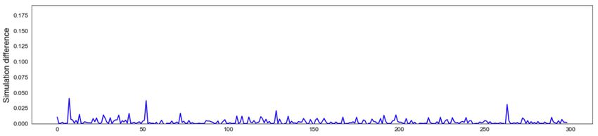
network is a research avenue for future study on interbank networks. The study
on the stability of the endogenously given structure is a necessary precondition
to understanding financial stability. Therefore, this research with an endoge-
nously formed network would enhance the literature on the Chinese interbank
market. Thirdly, to provide a more comprehensive analysis on the contagion
risk on the banking system in China, we extend the analysis further to lower
tiers of banks (Tier 3, 4, and 5, see Section 3), complementing previous studies
focusing on Tier 1 and 2 banks (Xie et al., 2016; Cao et al., 2017) only.
    The paper is structured in the following way. Section 2 provides a literature
review on the network formation, topology, and the interbank network in China.
Section 3 discusses the data, followed by the ABM methodology in Section 4.
Model validations are conducted in Section 5. The results of the contagion risks
are analyzed in Section 6, and Section 7 concludes the paper.

2     Literature Review
There is a growing number of researches concerning the financial networks’
contagion risk since the financial crisis in 2008 (c.f., Craig and Von Peter, 2010;
Gai and Kapadia, 2010; Anand et al., 2014). Financial institutions are highly
interconnected because they engage in a series of bilateral transactions, and
the interconnectedness makes the financial system very complex and difficult
to predict (Langfield and Soramäki, 2014). Much of the literature is devoted
to examining the relationship between the network connection and potential
contagion sources.
    Before the contagion effects of a given network can be evaluated, a question
comes first: how the interbank network is formed, which is the focus of our
paper.

2.1    Network Formation
Since bilateral transactions among banks are usually made over the counter,
and the information is not publicly available, it is challenging to model the
interbank network structure. The interbank network structure can be analyzed
using maximum entropy (Upper and Worms, 2004), minimum density (Anand
et al., 2014), and recently, the agent based models (Liu et al., 2020).
    Maximum entropy has been the leading method for researchers to construct
an interbank network. It uses a standard iterative algorithm to fill in the lia-
bility matrix’s blanks as evenly as possible, with available information on each
bank’s total interbank lending. It assumes that banks diversify their exposure
by spreading their lending and borrowing across all other active banks (Anand
et al., 2014). Many studies on interbank systemic risk are based on the ME
method (c.f. Upper and Worms, 2004; Wells, 2004; Van Lelyveld and Liedorp,
2006; Degryse and Nguyen, 2007; Upper, 2010; Boss et al., 2011; Mistrulli,
2011). However, the ME method has been criticized despite its popularity as
this method introduces bias (Mistrulli, 2011; Upper, 2011). As pointed out by

                                        3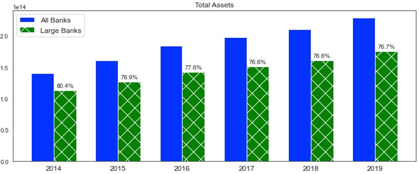
Mistrullie (2011), the ME method leads to an underestimation of the contagion
risk in magnitude and an overestimation of the scope of contagion by producing
too many links. A similar result is nuanced by Anand et al. (2014) in their
research using empirical data from the German interbank market.
     Anand et al. (2014) argue that banks would like to minimize the number
of necessary links for loan distribution based on the economic rationale that
interbank linkages are costly to add and maintain. Thus, Anand et al. (2014)
develop a minimum density approach to form a network. The approach iden-
tifies the most probable links and loads them with the most extensive possible
exposures consistent with each bank’s total lending and borrowing. Comparing
the network using MD with the actual interbank network from German, Anand
et al. (2014) find that the MD approach delivers an economically meaningful
alternative to ME and leads to a reasonable estimate of overall systemic risk in
the stress test. Although MD overestimates the contagion whereas ME under-
estimates it, using these two benchmarks helps identify a good range of possible
stress test results when the real counterpart exposures are unknown. Different
from solving a complex equilibrium for network formation, endogenous net-
work formation is another growing methodology for reconstructing links among
banks (Castiglionesi and Lavarro, 2011; Markose, 2012; Grasselli, 2013; Bluhm
et al., 2013; Halaj and Kok, 2014; Liu et al., 2018; Liu et al., 2020). Endoge-
nous network formation is related to agent-based modeling and game-theoretical
concepts (Halaj and Kok, 2014). The approach is usually related to optimiz-
ing specific issues, such as a portfolio return (Bluhm et al., 2014; Halaj and
Kok, 2014) or a lending-borrowing target (Liu et al., 2020). In Bluhm et al.
(2014), banks solve an optimal portfolio allocation problem by taking into ac-
count liquidity and capital constraints. With an iterative process to determine
the market price endogenously, and through the interactions of intermediaries’
borrowing and lending decisions, the interbank links emerge endogenously. In
Halaj and Kok (2014), banks allocate their interbank exposures while balanc-
ing the return and risk related to levels and volatility of market interest rates
and counterparty default risk, which results in a preferred interbank portfolio
allocation for each bank in the system. In Liu et al. (2020) model, banks set
their targets with specific interbank lending and borrowing ratios. The lending-
borrowing decisions are made for a bank based on the relationship scores and size
scores evaluated by the lending bank. Links for interbank lending are formed
endogenously through an iterative process that banks seek optimal status by
achieving interbank lending and borrowing target ratios.

2.2    Network Topology
Network topologies, such as core-periphery structure and power law distribution
of degree, are useful measures to gain insights into the real network (Boss et al.,
2004; De Masi et al., 2006; Soramäki et al. 2007; Bargigli, Iasio, Infante, Lillo
and Pierobon, 2013; Craig and von Peter, 2014; Fricke and Lux, 2015; Montagna
and Kok, 2016). Craig and von Peter (2014) introduce the core-periphery struc-
ture concept, where core banks form a complete network, and periphery banks

                                        4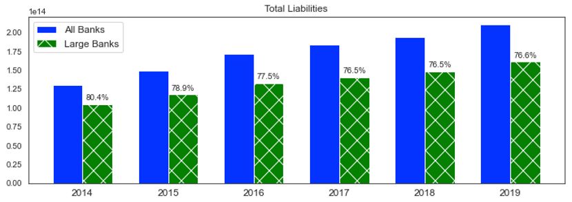
only link with core banks but not among themselves. Core banks play a cen-
tral role as intermediaries that hold together the interbank market. Empirical
studies confirm that some markets, i.e. the overnight interbank market in the
US, UK, Italy, etc, exhibit core-periphery structure (Soramäki et al. 2007; Iori,
De Masi, Precup, Gabbi and Cadarelli, 2008; Bech and Atalay, 2010; Langfield,
Liu, and Ota, 2014; Veld and van Lelyveld, 2014; Fricke and Lux, 2015a).
    The discussions on the degree distribution of nodes are controversial. Many
studies find that the interbank market’s network structure is scale-free (Boss et
al., 2004; De Masi et al., 2006; Alves, Stijin, et al., 2013; Léon and Berndsen,
2014). Since a scale-free network exhibits a power-law distribution of degrees,
it implies that there are very few banks with many interbank linkages, while
many banks have only a few links. However, the findings from Iori et al. (2008)
and Fricke and Lux (2015b) do not support the power-law distribution. Instead,
Fricke and Lux (2015b) find that negative binomial distributions best describe
the data. The scale-free banking system has also been coined robust-yet-fragile
(Haldane, 2009), indicating that random shocks are easily absorbed (robust).
In contrast, targeted attacks on the most central nodes may lead to a break-
down of the entire network (fragile). Thus, identifying systemically important
banks is crucial for policy objectives. Some algorithms are developed to mea-
sure banks’ importance, such as DebtRank (Battistonm, Puliga, Kashik, Tasca,
and Caldarelli, 2012), a novel measure of the systemic impact that inspired by
feedback-centrality and takes into account a recursive method. Another algo-
rithm is called SinkRank (Soramäki and Cook, 2013), a robust measure based
on absorbing Markov chains to model liquidity dynamics in payment systems.

2.3    Interbank Network in China
There is a growing number of studies on China’s interbank systemic risk in
recent years (c.f. Fei, Jiang, Zeng and Peng, 2016; Xie et al., 2016; Xu, He
and Li, 2016; Cao et al., 2017; Li, Liu and Wang, 2019; Li, Yao, Li and Zhu,
2019; Yang, Yu, and Ma, 2019; Zou, Xie, and Yang, 2019; Chen, Li, Peng and
Anwar, 2020; Sun, 2020). Some of these studies explore the systemic risks under
idiosyncratic shocks and systemic shocks scenarios (Fei et al., 2016; Li et al.,
2019; Chen et al., 2020). They find that China’s interbank network’s contagion
risk is minimal under an idiosyncratic shock, given any particular bank’s failure.
Similar results are nuanced by Xie et al. (2016) and Cao et al. (2017). However,
most of these studies use ME as a method for network formation (c.f. Fei et
al. 2016; Xie et al. 2016; Cao et al. 2017; Zou et al. 2019; Chen et al. 2019;
Sun, 2020), and it is known that this method generates too many links and
underestimates the contagion risk (Anand et al., 2014). Thus, it is necessary to
explore a method for a network that is closer to the real one in China.
    The study in the German interbank market by Anand et al. (2014) finds
that the actual network lies between the ones estimated by MD and ME. They
find the true network for German market is with density of 0.59%, it can be
described as a core-periphery structure where most of banks do not lend to each
other directly but through core banks acting as intermediaries. With a recent

                                        5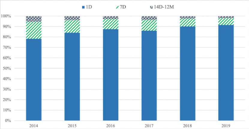
study by Liu et al. (2020) in the US market, an ABM approach can generate a
network between MD and ME.
   Therefore, in this paper, we use an ABM approach to estimate an interbank
network for China and compare the contagions for networks under ABM with
MD and ME.

3     Data
3.1    Interbank Market Participants in China
As shown in Table 1, there are four types of financial institutions (FIs) in China:
banks, securities companies, insurance companies, and other FIs (such as asset
management companies, financial leasing companies, etc.). Banks are the pri-
mary type of FIs with total assets of RMB 240,096 billion, accounting for 87.27%
of the total assets of all FIs, as of 2017. There are various types of banks in
China. Policy banks are unique since they are established to execute the gov-
ernment’s strategies in specific sectors and fund national projects not covered
by the fiscal budget (Chen, Mazumdar, and Surana, 2011). Due to these banks’
nature and the fact that they account for less than 10% of the financial indus-
try’s total assets, we exclude them in our study. Another significant type of
banks are state-owned banks, often referred to as the top tier commercial banks
in practice. According to the People’s Bank of China ("PBOC") 1 , there are
six state-owned banks: the Industrial and Commercial Bank of China, Bank of
China, China Construction Bank, Agricultural Bank of China, Bank of Com-
munications, and Postal Savings Bank of China. The state-owned banks have
average total assets of RMB16,971 billion, accounting for 37.01% of the finan-
cial industry. The three policy banks and six state-owned banks are classified
as Tier 1 banks. Twelve nationwide joint-stock commercial banks are classified
as Tier 2 banks, given their essential economic roles. They have total assets of
16.34% of the financial industry and average total assets of RMB3,747 billion.
    Tier 3 banks include 134 city commercial banks, and 39 foreign banks are
categorized as Tier 4 banks. Although foreign banks generally have strong
parent companies (or parent banks), their Chinese subsidiaries on a standalone
basis only have average total assets of RMB83 billion, a lot smaller compared
with that of RMB237 billion for the average total assets of city commercial
banks. Lastly, there are 1,262 rural commercial banks in the country. But they
only account for 8.6% of total assets of all FIs, with average total assets of
RMB19 billion. These rural commercial banks are classified as Tier 5 banks in
our study.
    There are 2,622 rural co-operative banks and credit unions categorized as
Tier 6 banks. They are not included in our study due to data availability and
the fact that they only account for 3.31% of total assets in the banking industry.
   1 http://www.cbirc.gov.cn/cn/view/pages/ItemDetail.html?docId=924532&itemId=863&generaltype=1,

last accessed on 15 September, 2020

                                         6
Table 1: Overview of financial institutions in China
Total Assets Institutions Avg Assets
Types of FIs Tiering
RMB, Bn % N RMB, Bn
(1) Banks
State-owned bank 101,827 37.01% 6 16,971
Tier 1
Policy bank 25,531 9.28% 3 8,510
Joint-stock commercial bank Tier 2 44,962 16.34% 12 3,747
City commercial bank Tier 3 31,722 11.53% 134 237
Foreign bank Tier 4 3,244 1.18% 39 83
Rural commercial bank Tier 5 23,703 8.62% 1262 19
Rural co-operative bank and credit union Tier 6 9,107 3.31% 2622 3
Banks - subtotal 240,096 87.27% 4078 59
(2) Securities Companies 6,140 2.23% 131 47
(3) Insurance Companies 16,938 6.16% 222 76
(4) Non-bank FIs 11,942 4.34% 437 27
Total 275,114 100% 4868 57
Note: This table shows an overview of different financial institutions in the
Chinese market. Banks are classified into six tiers. Source: Wind, based
on the results of 2017. RMB is the short form of the Chinese currency
Renminbi, and Bn stands for billion in this study.
3.2 Interbank Assets and Liabilities
The data are collected through the Wind database (Wind) from Wind Informa-
tion Technology Co. Ltd., one of China’s leading financial information service
providers. Our sample contains 299 banks with six consecutive years of financial
data for 2014 - 2019. As shown in Table 2, the sample includes six state-owned
banks (Tier 1), 12 joint-stock banks (Tier 2), 112 city commercial banks (Tier
3), 13 foreign banks (Tier 4), and 156 rural commercial banks (Tier 5). The
sample’s total assets are RMB 197,732 billion, representing 82.4% of the entire
banking industry in 2017.
We collect the key financial data from the banks’ annual financial results
from 2014 to 2019 to construct a stylized financial statement, as illustrated in
Table 3. In our study, interbank assets include interbank lending and deposits
to other banks, while the interbank liabilities include interbank borrowing and
deposits from other FIs. External assets are calculated as the difference between
total assets and interbank assets. External liabilities are the differences between
total liabilities and interbank liabilities.
In an interbank network that consists of all participants, the sum of interbank
assets should equal the sum of interbank liabilities. Since our sample data do not
include all FIs, particularly without the non-banking FIs, the sum of interbank
assets and the sum of interbank liabilities are not equal, as shown in Table 4.
The sum of interbank liabilities is higher by 57.12% than the sum of interbank
assets. Interbank liabilities are from banks and other non-bank FIs, which
7Table 2: Overview of bank tiers
% of the total assets of
Tier Bank type Number of institution
the sample
Tier 1 State-owned banks 6 54.00%
Tier 2 Joint-stock banks 12 23.37%
Tier 3 City commercial banks 112 15.68%
Tier 4 Foreign banks 13 0.85%
Tier 5 Rural commercial banks 156 6.10%
Total 299 100%
Note: This table shows our sample data, including 299 banks within five dif-
ferent tiers. Source: Wind, and compiled by the author, based on the
financaial results of 2017.
Table 3: Illustration of a stylized balance sheet
Interbank assets Interbak liabilities
Interban lending-borrowing Interbank borrowing
Deposit to other banks Deposit from other FIs
External assets External liabilities
Total equities
Total assets Total liabilities and equities
Note: This table shows the critical items of data used in our analysis. In-
terbank assets comprise interbank lending and deposits to other banks,
and interbank liabilities consist of interbank borrowing and deposits from
other FIs. All the table items are collected, except external assets, and
external liabilities are calculated according to the formulas: external as-
sets = total assets – interbank assets, external liabilities = total liabilities
– interbank liabilities.
8Table 4: Aggregation of interbank assets and liabilities
Sum of Sum of Reduction
Percentage
Year interbank interbank Ratio
(“IA/IL”)
assets (“IA”) liabilities (“IL”) (1-IA/IL)
2014 8,422.92 17,603.85 47.85% 52.15%
2015 9,036.19 22,260.68 40.59% 59.41%
2016 10,175.72 23,272.60 43.72% 56.28%
2017 8,407.51 21,397.32 39.29% 60.71%
2018 8,986.81 20,980.01 42.84% 57.16%
2019 9,404.99 21,439.38 43.87% 56.13%
Average 9,072.35 21,158.97 42.88% 57.12%
Note: This table shows the sum of interbank assets and liabilities for 299 banks
in our sample. The sum of interbank liabilities is greater than the sum
of interbank assets by 57.12%. Therefore, this excess portion is to be
reduced, assuming it is the portion of interbank liabilities from other non-
bank FIs which are not included in our study. The data are in billion
RMB except for ratios.
implies the excess portion of 57.12% (on average) is interbank liabilities from
non-bank FIs. Thus these portions of amounts should be excluded from the
data for interbank liabilities. Therefore, we calculate the reduction ratio for
each year, as shown in Table 4, and reduce the interbank liabilities for all the
banks on a pro-rata basis to achieve equal status for the sum of interbank assets
and liabilities.
To check whether the above reduction ratio is an appropriate portion of in-
terbank liabilities for non-bank FIs, we break the interbank liabilities down into
two parts, interbank liabilities from banks and interbank liabilities from other
non-bank FIs. However, not every bank has reported these numbers separately.
Thus we collect numbers from 11 large banks (defined in Section 3.3) that are
publically available for proximation. We calculate the portion of interbank li-
abilities from other non-bank FIs, based on the data collected for 2019. As
depicted in Figure 1, the average ratio is 66.62%, close to the ratio of 56.13%
for 2019 in Table 4. Therefore, we use 56.13% as a reasonable estimation.
It is also noticeable that a few banks in our sample do not participate in the
interbank market, as shown in Table 5. For example, in 2019, 3 banks do not
have interbank assets, nine banks do not have interbank liabilities, and three
banks have neither interbank assets nor interbank liabilities. As a result, these
three banks become isolated nodes. Thus, the number of nodes in the connected
network for 2019 should be 296, instead of 299.
3.3 Large and Small Banks
Large banks are less prone to default risk, and small banks rely on large banks
when borrowing funds. Therefore large and small banks behave differently in
9Figure 1: Ratios of interbank liabilities from non-bank FIs. This figure shows
the portion of interbank liabilities from other non-bank FIs for the selected 11
banks based on the financials of 2019. The ratio ranges from 37.12% to 82.34%,
with an average of 66.62%.
Table 5: Number of banks without interbank assets and liabilities
2014 2015 2016 2017 2018 2019
Without interbank assets 6 2 1 2 0 3
Without interbank liabilities 20 10 8 9 6 9
With neither 6 2 1 2 0 3
Note: This table shows the number of banks without interbank assets or li-
abilities for 2014-2019. The banks identified with neither are considered
isolated nodes in the network, not connected to any other banks in that
year. Thus, the number of the nodes in that year should be the total
number of banks minus the number of these isolated nodes.
10Figure 2: Cumulative distribution function for shares of total assets of banks in
2019. This figure shows the cumulative distribution function for the share of each
bank’s total assets as a percentage of all banks. The banks are ranked in order
by their shares from the largest to the smallest and then plot the cumulative
distribution function. For instance, the first dot in the figure represents the
largest bank’s share; the second dot represents the cumulative shares of the 1st
and 2nd largest banks, and so on.
the interbank market (c.f. Upper, 2011; Lux, 2015; Liu et al., 2020). We rank
the banks in our sample by their market shares from the largest to the smallest
and then plot the cumulative distribution function, as shown in Figure 2. The
cumulative distribution function is defined as:
F (xi ) = f (X ≤ xi )
where F (xi ) is the cumulative distribution function, and f (xi ) is the proba-
bility density function. The slope of the function is very steep before it reaches
80%, and afterward, the curve becomes flattened, implying that a small number
of banks account for 80% of the total shares and the remaining banks account
for the rest 20%. Therefore, we classify the banks that composite the top 80%
market shares as large banks. We plot this function for each year for six con-
secutive years from 2014 to 2019 and repeatedly identify the banks within the
top 80% for each year. It is noticeable that 16 banks are present every year.
Therefore, these 16 banks are defined as large banks, while the rest are defined
as small banks.
Table 6 lists the large banks, including six state-owned banks, nine joint-
stock banks, and one city commercial bank. The proportions of large banks’
total assets range from 76.7% to 80.4% for 2014 – 2019, as shown in Figure 3.
In 2019, large banks account for 76.7% of the total assets, 76.6% for the total
liabilities, 75.2% for the interbank assets, and 82.1% for the interbank liabilities.
We compare large banks and small banks for their interbank asset ratios
and interbank liability ratios for 2014 - 2019. Table 7 shows that the average
11Table 6: The list of large bank
Type Name
Industrial and Commercial Bank of China Ltd (ICBC)
Bank of China Ltd (BoC)
State-owned bank (6) China Construction Bank Corporation (CCB)
Agricultural Bank of China Ltd (ABC)
Bank of Communications Co Ltd (BoCom)
Postal Saving Bank of China Co Ltd (PSB)
China Guangfa Bank Co Ltd (CGB)
PianAn Bank Co Ltd (PAB)
China Everbright Bank Co Ltd (CEB)
China Merchants Bank Co Ltd (CMB)
Joint-stock bank (9)
China Minsheng Banking Corp Ltd (Minsheng)
China Citic Bank Corp Ltd (Citic)
Shanghai Pudong Development Bank Co Ltd (SPD)
Industrial Bank Co Ltd (IB)
Hua Xia Bank Co Ltd (HXB)
City commercial bank (1) Bank of Beijing Co Ltd (BoBJ)
Note: This table shows the list of large banks in our sample, including six
state-owned banks, nine joint-stock banks, and one city commercial bank.
Their abbreviations are listed in brackets.
12(a) Total assets
(b) Total liabilities
Figure 3: Comparison of the Total Assets and Total Liabilities between Large
and All Banks. These figures show the comparisons of the total assets (a) and
total liabilities (b) for the large banks, and for all banks, the shares of the large
banks’ total assets range from 76.7% to 80.4% for 2014-2019, and the shares of
the large banks’ total liabilities range from 76.5% to 80.4% for 2014-2019.
13Table 7: Interbank asset-liability ratios between large and small banks
Interbank asset ratio Interbank liabilitiy ratio
Year
Large- Small- t p- Large- Small- t p-
mean mean value mean mean value
2014 5.67% 10.04% 4.92 0.0000 8.35% 4.09% 4.25 0.0005
2015 4.50% 2.97% 2.12 0.0456 5.19% 2.59% 4.12 0.0007
2016 4.93% 4.22% 2.24 0.0329 6.17% 3.12% 3.75 0.0016
2017 3.78% 4.80% 3.10 0.0034 5.49% 2.76% 3.58 0.0023
2018 3.69% 4.62% 3.18 0.0025 5.49% 2.66% 4.37 0.0004
2019 3.45% 4.05% 2.32 0.0236 4.99% 2.00% 5.88 0.0002
Average 4.34% 5.12% 5.94% 2.87%
Note: This table compares the interbank asset-liability ratio between large
banks and small banks. As the table shows, large banks, on average,
have smaller interbank asset ratios than small banks. Still, in contrast,
large banks have large interbank liability ratios on average than small
banks. The interbank liabilities have already been reduced according to
the procedure described in Section 3.2.
interbank asset ratio for 2014 - 2019 for large banks is 4.34%, slightly lower than
5.12% for small banks, which implies small banks have more significant needs to
lend. Large banks have an interbank liability ratio of 5.94%, more than double
than 2.87% of small banks, which implies large banks absorb more liabilities
from the interbank market and lend to external markets outside the interbank
network. The means of both interbank asset ratio and interbank liability ratio
for 2014 – 2019 between large and small banks have been tested by using a
Welch t-test method. The mean differences for each year are all significant at
the 5% level.
Based on our analysis, it is clear that large and small banks’ characteristics
are substantially different, leading to different lending and borrowing behavior
as agents.
4 Model and Methodology
4.1 Eisenberg-Noe Clear Payment Vector
In the interbank network, nodes represent banks, and directional edges represent
the claim of node i to node j . Eisenberg and Noe (2001) start by denoting L
as liabilities, eas cash flow, and p as payment. So Lij is the liability of node i
to node j . Denote pi as all payments of node i, thus
n
X
p¯i ≡ Lij
j=1
14Q
Let ij denote the liability matrix, which captures the proportion of pay-
ment from node i to node j as the total payments of node i. We have
(L
ij
Q p¯i if p¯i > 0
ij ≡
0 otherwise
We assume that all debt claims have
Q equal priority. As a result, the payment
from node i to node j is equal to p¯i ij , and the total payments received by
Pn QT
node i is equal to j=1 ij pj . The total cash flow received by node iequals
the sum of Pthe payments received by other nodes plus the operating cash flow,
N QT
denoted as j=1 ij pj + ei . The mechanism sets three criteria in the clearing
process, which are:
1. Limited liability. a bank could pay no more than its available cash flow;
2. The priority of debt. Stockholders of a bank receive no value until it pays
off its outstanding liabilities;
3. Proportionality. If a default occurs, creditors are paid in proportion to
the size of their nominal claim on the defaulted bank’s assets.
To establish a fixed-point characterization, the payment vector p∗i ∈ [0, p] is the
clearing payment vector if and only if the following condition holds for ∀i ∈ N :
h Pn QT i
p∗i = min ei + j=1 ij p∗j , p¯i
and the equity value of node expressed as would be
Pn QT
Vi = j=1 ij pj + ei − pi
The simulations of default are generated using the following steps:
Step QT assume pi = p¯i to calculate the net value of bank isuch that
Pn1: we
Vi = j=1 ij pj + ei − pi . If all Vi s are positive, it means that no bank
defaults and the algorithm terminates. Otherwise, go to Step 2.
Step 2: Banks with a net value Vi < 0 can only pay part of their liabilities
to other creditors. The partial payment ratio is
PN QT
j=1 ij p j + ei
θi =
pi
Under the assumption that only these banks default, we replace Lij with
θi LijQso that the limited liabilities criterion is met. Thus we get a new set of
Lij , ij , pi , and Vi .
Step3: we repeat Step 2 until no more bank defaults.
15Figure 4: The iterative process of our ABM. In each cycle (a cycle is defined as
a year in this study), all the banks undergo three processes, paying outstanding
debts, settling new debts, and updating financial statements, and these processes
are reiterated for the next cycle.
4.2 An ABM Approach for Interbank Network Formation
Agent-based modeling is an approach to modeling complex systems composed
of interacting, autonomous ‘agents.’ Agents have behaviors described by simple
rules and interact with other agents, influencing their behaviors (Macal and
North, 2010). According to Macal and North (2010), a typical ABM comprises
of three elements, (1) a set of agents, their attributes and behaviors; (2) a
set of agents’ relationships and methods of interactions; and (3) the agents’
environments, where agents interact with in addition to other agents. Our
ABM is also an iterative simulation process, as illustrated in Figure 4. Each
fiscal year is treated as a business cycle. All agents (banks) perform the following
three actions step by step: paying outstanding debts, settling new debts, and
updating financial statements. At the beginning of time t, agents pay all their
outstanding debts for the previous period t − 1 before borrowing new debts.
After all debt payments are cleared, agents begin to settle new debts for the
period according to rules set out in Section 4.2.2. Once the process of settling
new debts has been completed, the banks update financial statements for the
period t to reflect the established interbank assets and liabilities from the new
debt settlement process. These processes are iterated into the next cycle t + 1,
and so on.
4.2.1 Paying Outstanding Debts
All interbank loans in China are within a 1-year term, according to the statistics
from Wind. Figure 5 shows the composition of interbank lending by different
tenors. The majority of the interbank loans are within 1-day (91.42% in 2019)
and 7-days (6.62% in 2019) tenors. Since the interbank loans are short-term,
it is assumed all agents must pay their existing debts at the beginning of each
cycle before they can request new borrowings from other counterparties. An
Eisenberg-Noe clearing payment vector method is applied for paying outstand-
ing debts. If an agent fails to meet all its obligations, its creditors’ equity loss
would be applied. The repayment received by each creditor is calculated on a
pro-rata basis according to the payment vector. A bank will bankrupt if the
losses incurred for its share are larger than its equities. Following Liu et al.
(2020), we estimate the interbank network using the ME method to construct
an initial network. After that, each year’s interbank network is formed through
16Figure 5: Composition of the tenors for interbank loans. Composition tenors
for interbank loans in the percentage of each year for 2014 – 2019. The tenors
contain 1-day, 7-days, 14-days to 12-months (collectively shown as 14D-12M).
As shown, the majority of interbank loans are with a tenor of 1-day and 7-days.
The source is from Wind.
the ABM approach with the process described in Section 4.2.2. After all the
debts are cleared, all the banks’ financials are updated to settle new debts.
4.2.2 Settling New Debts
The process of settling new debts is carried out according to the following rules.
Each bank sets its target ratios for interbank lending and borrowing at the
beginning. Based on these ratios, every bank can determine their annual target
interbank lending-borrowing amounts. Banks that have not met their target
borrowing ratios would start to make borrowing requests to other banks. The
borrowing requests are first made to large banks. A borrowing bank selects
a large bank at random to request borrowing for the residual amount. If the
lending bank does not fulfill the demanding borrowing amount, the borrowing
bank will request the next large bank until its borrowing needs are fully met.
Suppose that the borrowing needs are not fully met after going over all the
large banks. The borrowing bank will then send a request to small banks with
previous borrowing relationships within the relationship score’s ranking order.
Each bank evaluates its relationship with other banks with a relationship score.
The relationship score captures a bank’s tendency to keep existing relationships
(Liu et al., 2020), and it is calculated as:
17
log(debts),
if i and j have bilateral debts
R R
Si,j (t) = ηSi,j (t − 1), else if t > 0
0, otherwise
R
where Si,j (t) is the relationship score of bank j evaluated by bank i in period
t. The debts in this study contain two bilateral debts between i and j, which
means that there are the debts for bank i to j and debts from j to i if both
directions exist. η is the memory decaying factor parameter, which is set at 0.9
by default, according to Liu et al. (2020).
If the borrowing needs are still not wholly fulfilled after gone over all the
relationship banks, the borrowing bank will continue to send requests to the rest
of the small banks in the order of the size score. The size score is to capture
the preference of banks to do business with larger banks which are with more
assets; it is calculated as:
P
S k,k6=i logAk (t − 1)IIi,k (t − 1)
Si,j (t) = logAj (t) − P
k,k6=i IIi,k (t − 1)
where
(
1, if i and k have a relationship in period t
IIi,k (t) =
0, otherwise
S
Si,j (t) is the size score of bank j evaluated by bank i in period t, Aj (t) is
the total assets of bank j at time t, and IIi,k (t) is the binary variable to keep
track of previous debt obligations. The borrowing process would be terminated
either when the borrowing bank meets its predetermined borrowing target or
when there is still an unfulfilled gap after going over all the other banks.
On the lending side, when a lending bank receives a borrowing request from
a borrower, it needs to make two decisions, whether to lend and how much if it
decides to lend. The question of lending or not is a binary classification problem.
The lender follows a sigmoid function for its decision-making process. The lender
evaluates a borrower with a total score, which combines the relationship score
and the size score, and it is calculated:
T S R
Si,j (t) = ω × Si,j (t) + (1 − ω) × Si,j (t)
T
where Si,j (t) is the total score that i assigns to j in period t, which is a
weighted average of the relationship score and size score that i assigns to j for
the same period. ω is the weighting parameter, set to be 0.5 by default (Liu
et al., 2020). The lender uses a sigmoid function to calculate the probability of
lending to the borrower:
T 1
P Si,j (t) = T (t)
1 + α · exp β · Si,j
18Figure 6: Sigmoid function for the relationship between the total scores and the
lending probability. This sigmoid function shows the relationship between the
total scores (x-axis) and the lending probability (y-axis). The blue dash line is
plotted with α for U (0.9, 1.1) and β for U (−1.1, −0.9). Therefore, the lending
probability equal to 0.5 when the total score is 0. The solid green line is plotted
with α for U (0.0, 0.1) and β for U (−1.1, −0.9), the lending probability equal to
0.5 when the total score is -2.8. Compared with the blue line, the green line’s
function would encourage the banks to lend at a lower total score.
T
where P Si,j (t) is the probability that i lending to j, and α and β are
two parameters controlling the intercept and slope, respectively. Here α and
β are chosen from uniform distributions U (0.0, 0.1) and U (−1.1, −0.9). These
parameters have been adjusted (see Section 5.2 for detail) to match the Chi-
nese banking market’s interbank lending situation (see Figure 6). The cut-off
threshold for the
Tprobability
is set to be 0.5, which means bank i will only lend
to bank j if P Si,j (t) ≥ 0.5.
Once the lending bank decides to lend, the lending amount is to be de-
termined upon three numbers. Firstly, the amount that the lender decides to
lend by following a uniform distribution to determine a fraction from its initial
target lending limit; secondly, the available lending amount at the time being
requested; and thirdly, the requested amount from the borrower. The lowest
number would be chosen as the lending amount for the transaction. The trans-
action detail consists of two counterparties and a transaction amount, recorded
as an edge-list item to construct the interbank network.
4.2.3 Update Financials
After the lending and borrowing processes for all banks are completed, each
bank would have one or more interbank transactions with its counterparties.
We obtain a full edge-list of transaction details for constructing a network of
interbank lending. If a bank has no lending or borrowing transaction, it will
become an isolated node in the network. The total amount of interbank lending
19and interbank borrowing for all banks have been recorded to update the stylized
balance sheet’s financial items for the same period. Total assets, total liabilities,
and total equities are drawn from empirical data, and the external assets and
external liabilities are inferred accordingly, as shown in Table 3. The updated
balance sheet and the interbank network are served as inputs for the next period
for clearing the outstanding payments.
5 Model Validation
5.1 Parameter Adjustment
Different αs have different impacts on lending probability. Thus, we try different
values for α to minimize simulation error, which is calculated as:
v
uX r (t) − rE (t) 2 × T Ai (t)
u n s
L i i
Error (t) = t Pn
t i T Ai (t)
P2019
ErrorL (t)
Average− errorL = t=2015
m
v
uX r (t) − rE (t) 2 × T Li (t)
u n s
B i i
Error (t) = t P n
t i T Li (t)
P2019
ErrorB (t)
Average− errorB = t=2015
m
where ErrorL (t) and ErrorB (t) are simulation errors of interbank lending
and interbank borrowing at time t, respectively. ris (t) is the simulated ratio for
bank i at time t, which is compared with its empirical ratio riE (t). T Ai (t) and
T Li (t) are the total assets and total liabilities of bank i at time t, respectively.
n is the total number of banks, which is 299 in this case. Average− errorL and
Average− errorB are the average simulation error for lending and borrowing
for 2015 - 2019. m is the number of years for the simulation, five years in
our sample. We run different simulations with different αs from the uniform
distribution of the following 19 intervals, U (0.0, 0.1) to U (0.9, 1.0) with interval
maintaining at 0.1 and incremental of 0.05 for each step. The simulated average
errors for both lending and borrowing ratio are shown in Figure 7.
To select an α with the lowest error for both lending ratio and borrowing ra-
tio, we calculate a total error that takes into consideration both Average− errorL
and Average− errorB :
q
T otal− error = (Average− errorL )2 + (Average− errorB )2
We repreat the above simulation for 30 times, and obtain 30 different total− errors
for each a value. In addition, we calculate the average total− error for each α
20Figure 7: Plot of simulated average errors for lending ratio and borrowing ratio.
This figure shows the plot of the simulation errors for Average− errorL (solid
blue) and Average− errorB (deshed green) under different values for α selecting
from 19 different uniform distributions begin with U (0.0, 0.1) with incremental
of 0.05 up to U (0.9, 1.0). The X-axis represents different α values, and the y-axis
represents the simulated average errors. The lowest simulation errors for both
ratios are annotated respectively, with the red circles in the figure.
Figure 8: This figure shows the average total− error for each α value of the 30
simulation results. As the figure shows, the lowest average total− error is found
when α is chosen from U (0.0, 0.1).
value based on the 30 times simulation results, as Figure 8 shows, the lowest
average total− error is found when αis chosen from U (0.0, 0.1), thus U (0.0, 0.1)
is used as the uniform distribution interval in our model for the a value.
According to the method and parameters described above, an interbank
network is endogenously formed. The network is drawn in Figure 9.
5.2 Target Ratio Validation
We use the data of 2014 with the ME method to estimate an initial network
and iterate the simulation process described in Section 4 from 2015 to 2019.
We compare the target lending and borrowing ratios between the simulation
results and empirical data for 2019, as shown in Figure 10. The distributions of
lending and borrowing ratios of the simulated data are closed to the empirical
data. Figure 11 shows the differences between the simulation and the empirical
of each bank’s lending and borrowing ratios. The comparison of the simulated
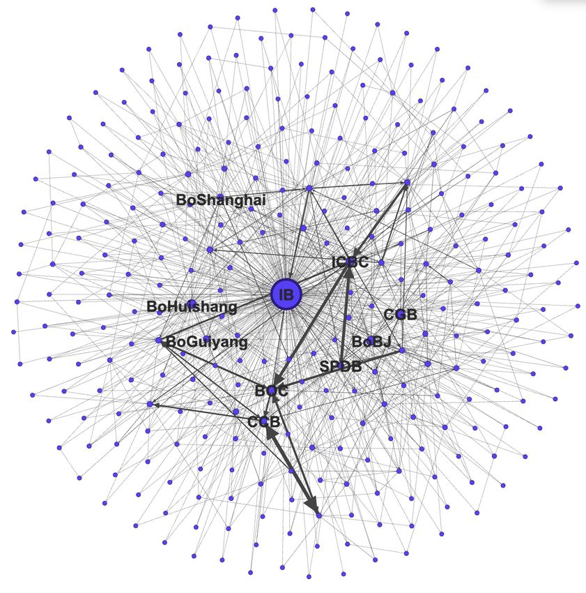
21Figure 9: Interbank network representation formed by the ABM approach for
China. This figure shows the interbank network representation based on 2019,
formed by the ABM approach. The sizes of the nodes are weighted by their
degrees. The links are weighted by the size of the bilateral lending. Names for
nodes with degrees over 20 are shown. The graph is drawn using an open-source
software Gephi with Fruchterman Reingold layout.
22(a) Interbank lending ratio for 2019 (b) Interbank borrowing ratio for 2019
Figure 10: Comparison of lending and borrowing ratios distributions between
simulation and empirical. These figures compare the histogram distributions
for the simulated results with the empirical data for both the interbank lending
ratio (a) and the interbank borrowing ratio (b) for 2019. The histograms are
plotted with 20 bins.
data with empirical data demonstrates a close estimation made by our ABM
approach.
5.3 Interbank Network Formation Comparison
Following the approach described in the model section, an interbank network is
formed and iterated until 2019. The network for 2019 under ABM is compared
with that using MD and ME. Empirical data show three small banks without
interbank assets nor interbank liabilities, as shown in Table 5, which implies that
they do not participate in interbank lending nor borrowing. Thus these banks
would be isolated from the connected network. Therefore, they are excluded
when making network properties comparison. Our ABM network can identify
these three isolated nodes (see Table 5) so that the simulated network is with 296
banks, consistent with the results from the MD and ME. A comparison among
MD, ABM, and ME network for their characteristics with selected features are
shown in Table 8.
The degree, calculated by the sum of in-degree and out-degree, measures how
many node links have. The ABM network’s average degree is 3.00, which lies
between the 2.15 of the lower bound for MD and 289.02 of the upper bound for
ME. For the ABM network, 90% of the banks have less than ten links, consistent
with the US interbank network (Liu et al., 2020).
Degrees of the interbank network for many markets have been reported to
exhibit a power-law distribution (Boss et al., 2004; De Masi et al., 2006; Alves,
Stijin, et al., 2013; Léon and Berndsen, 2014). Figure 12 shows the power-
law fit of the degrees for MD, ABM, and ME networks. The result supports the
finding of a scale-free structure network. The power-law distribution component
for MD, ABM, and ME networks is found to be 1.97, 2.47, and 2.45, respectively.
23(a) Interbank lending ratio
(b) Interbank borrowing ratio
Figure 11: Differences between the simulation with empirical for each bank.
These figures show the differences between the simulated results with the em-
pirical data for the interbank lending ratio (a) and interbank borrowing ratio
(b) for each bank based on 2019.
Table 8: Comparison of network properties under different approaches
Properties MD ABM ME
Number of nodes 296 296 296
Number of edges 636 889 85,550
Average degree 2.15 3.00 289.02
Graph density 0.007 0.010 0.98
Power law exponent 1.97 2.47 2.45
Average clustering coefficient 0.163 0.144 0.98
The average shortest path length 3.919 3.967 1
Note: This table compares the network properties for networks constructed
with MD, ABM, and ME using data of 2019. The MD and ME are es-
timated using R with a package, namely NetworkRiskMeasures (v-0.1.2).
The properties are measured using the networks, excluding the isolated
nodes. Calculations of network properties (except power-law exponent
using Python with package namely power-law developed by Alstott, Bull-
more, and Plenz (2014)) are made with an open-source software Gephi.
24Figure 12: Cumulative degree distribution on a double log scale. The figure
displays the degree distribution in its cumulative form, showing the number of
banks with a degree greater than the number shown on the x-axis on a double
log scale. The estimations of alpha and xmin and the plot are processed in
Python with a package of powerlaw v-1.4.6 (Alstott, Bullmore and Plenz, 2014)
using discrete data method.
Network density describes the portion of the potential connections in a net-
work that are connected. ABM’s density is 0.010, slightly higher than that for
MD of 0.007, but vastly lower than that for ME of 0.98. The clustering co-
efficient is the propensity of nodes to form cliques. ABM’s average clustering
coefficient is at 0.144, lower than the MD and ME, which are 0.163 and 0.98,
respectively. The shortest path length measures the number of steps for any
given node to reach any other network nodes. ABM and MD are similar to
3.967 and 3.919, respectively. Still, ME only has 1 step for the shortest path
length; it means any two nodes are connected, unrealistic in many markets.
In general, except for the component of the power-law distribution of de-
grees, we find many network property measures for ABM, i.e., number of edges,
average degree, graph density, lie between MD and ME, which nuances the
similar finding of Anand et al. (2014) and Liu et al. (2020). For the average
clustering coefficient and the average shortest path length, ABM is close to MD.
ME network is far away from both ABM and MD, which suggests that ME is
far from generating a realistic interbank network in China.
6 Simulation of Credit Shocks and Contagion Risks
Following Sun (2020), we define a bank’s failure, or bankruptcy, as occurring
when a bank’s losses in assets exceed its net worth, and the net worth in this
study is measured by a bank’s total equity, which is obtained from the bank’s
financial statement.
25Table 9: Contagion risk: the causes and consequences
Cause Consequence
Defaulting banks N Affected banks by tiers
Rural commercial bank (5)
IB 7
Foreign bank (2)
ICBC 2 Foreign bank (2)
Foreign bank (1)
CGB 2
Rural commercial bank (1)
BoBJ 1 Rural commercial bank (1)
Rural commercial bank (7)
Total 12
Foreign bank (5)
Note: This table shows the simulation results of idiosyncratic shock. Based
on the results, the defaults of 4 banks would cause 12 other banks to fail.
The affected banks are 7 rural commercial banks and 5 foreign banks.
6.1 Simulation of Credit Shock
To understand each bank’s systemic importance within the network, we assess
the contagion risk of each bank’s default on causing other banks’ failures through
the interconnected network. Following the Eisenberg-Noe clear payment algo-
rithm, we simulate the contagion result by assuming one bank default at a time,
in particular, by assuming a 100% loss ratio of external assets (Sun, 2020). Un-
der this scenario, we explore the consequence of the number of other banks are
affected to fail. The simulation results based on the network of 2019 are summa-
rized in Table 9. It is found that 4 banks’ defaults cause 12 other banks to fail.
The causing banks include one state-owned bank (ICBC), two joint-stock banks
(IB, CGB) and one city commercial bank (BoBJ). IB has the highest number
of degrees in the network. Its default causes 7 other banks to fail, including 5
rural commercial banks and 2 foreign banks. ICBC’s default causes 2 foreign
banks’ failures. CGB’s default causes a failure of a foreign bank and a rural
commercial bank, and BoBJ’s default causes a rural commercial bank to fail. In
summary, within the 12 affected banks, 7 of which are rural commercial banks,
and the remaining 5 are foreign banks . We further analyze the second round
of shocks by the failures of the affected banks and find out no more other banks
are caused to fail.
6.2 Robustness Check
The credit shocks simulation results by Cao et al. (2017) suggest no systemic
risk in China’s interbank market. A similar result was nuanced by Sun (2020),
which finds that even the default of ICBC, the world’s largest bank in terms of
assets, will not cause any other bank failure. Both Cao et al. (2017) and Sun
(2020) use the ME method to estimate the interbank network, which leads to
26Figure 13: Affected banks fail frequency per 30 times simulations. This figures
shows 35 banks fail during the 30 times repeated simulations. The affecting
banks are ranked in decending order of the number of times fail per the 30
times simulations. As shown, 31 out of 35 banks fail respeatedly at least twice
or more.
a bias of the contagion risk. In contrast, our simulation results do not support
the findings of Cao et al. (2017) and Sun (2020). Our simulation result of credit
shocks shows that the defaults of 4 banks cause another 12 banks’ failures based
on the simulated network for 2019. In addition, based on the 30 times repeated
simulations as described on Section 5.1, the results shows that there are 35
banks fail for 478 times in total, and some banks are consistently found to fail.
For instance, a bank is found to fail 37 times during 30 times simulations, and
within some simulations it fails more than once since more than one causing
bank could lead to its failure. Figure 12 plots the number of times that banks
fail in a ranking order. In terms of analysis of the failing banks by their bank
tiers, despite 4 city commercial banks are found to fail 42 times for the 30
times simulations, foreign banks and rural commercial banks are found to fail
more frequently, more specifically, 12 foreign banks fail 203 times, and 19 rural
commercial banks fail 233 times, as Table 10 shows. The 30 times simulations
results are consistent with the findings of Section 6.1, where rural commercial
banks and foreign banks are more fragile to the credit shocks.
6.3 Policy Implications
To explore why banks are affected to fail and make suggestions for policymakers,
we examine whether the defaulting banks are due to excessive interbank lending
and over-concentration of interbank lending. We measure the excessiveness of
interbank lending by a ratio of a bank’s interbank asset over its total equity,
27Table 10: Statistics of affecting banks for the 30 times simulations
Bank tier No. of banks failing No. of times of failing
City commercial bank 4 42
Foreign bank 12 203
Rural commercial bank 19 233
Total 35 478
Note: The table shows the statistics of the affecting banks by bank tier. There
are total 35 banks are affected to fail, of which 4 are city commercial banks,
12 are foreign banks and 19 are rural commercial banks. In terms of the
number of times of failing, foreign banks and rural commercial banks fail
203 and 233 times , respectively, out of the total failing times of 478 for
the 30 times simulations.
which is defined as:
interbank− asseti
ILERi =
total− equityi
where ILERi is the interbank lending excessiveness ratio for bank i. On
the other hand, the over-concentration of interbank lending is measured by a
bank’s interbank assets from its largest borrower as a proportion of the bank’s
total interbank assets, which is defined as:
interbank− assets− f rom− largest− borroweri
ILCRi =
total− interbank− assetsi
where ILCRi is the interbank lending concentration ratio for bank i.
Figure 14 shows a scatter plot of the lending excessiveness ratio and lend-
ing concentration ratio. As Figure 14 shows, the defaulting banks (marked as
crosses) are located in the upper right corner, indicating the defaulting banks
have high lending excessiveness ratios and high lending concentration ratios. We
compared the ILERs between the defaulting banks and non-defaulting banks.
The average ratios are found to be 1.83 and 0.38,the mean difference is sig-
nificant at 0.0000 level by a Welch’s t-test. The ILCR for the defaulting and
non-defaulting banks are found to be 0.82 and 0.73, respectively, which does not
appear a statistical significance (p-value at 0.1673). We perform a revers check
for the ratios for 2015-2018, the result is shown in Table 11. It is found that
the mean difference for ILER is consistently significant, but not ILCR.
Given the significance of ILER, we continue to compare this ratio among
different tiers of banks. As shown in Figure 15, foreign banks are among the
top of the list, with an average ratio of 1.65. It means that foreign banks, on
average, with the sizes of exposures to interbank risks exceeding their respective
total equities, which implies they have a higher probability of being affected to
fail by the credit shocks. It is recommended to the policymakers to consider
28You can also read