ELF: Embedded Localisation of Features in pre-trained CNN
←
→
Page content transcription
If your browser does not render page correctly, please read the page content below
ELF: Embedded Localisation of Features in pre-trained CNN
Assia Benbihi1,2 , Matthieu Geist3 , and Cédric Pradalier1,4
1
UMI2958 GeorgiaTech-CNRS
2
Centrale Supélec, Université Paris Saclay, Metz
3
Google Research, Brain Team
4
GeorgiaTech Lorraine
arXiv:1907.03261v1 [cs.CV] 7 Jul 2019
Abstract
This paper introduces a novel feature detector based only
on information embedded inside a CNN trained on stan-
dard tasks (e.g. classification). While previous works al-
ready show that the features of a trained CNN are suit-
able descriptors, we show here how to extract the feature
locations from the network to build a detector. This in-
formation is computed from the gradient of the feature
map with respect to the input image. This provides a
saliency map with local maxima on relevant keypoint lo-
cations. Contrary to recent CNN-based detectors, this
method requires neither supervised training nor finetun-
ing. We evaluate how repeatable and how ‘matchable’ the
detected keypoints are with the repeatability and match-
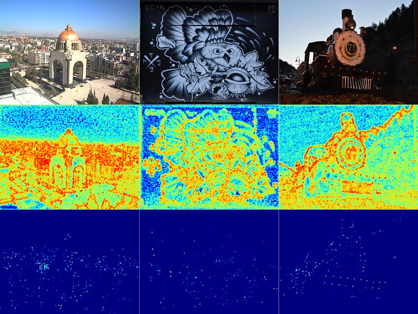
ing scores. Matchability is measured with a simple de- Figure 1: (1-6) Embedded Detector: Given a CNN trained
scriptor introduced for the sake of the evaluation. This on a standard vision task (classification), we backpropa-
novel detector reaches similar performances on the stan- gate the feature map back to the image space to compute
dard evaluation HPatches dataset, as well as comparable a saliency map. It is thresholded to keep only the most in-
robustness against illumination and viewpoint changes on formative signal and keypoints are the local maxima. (7-
Webcam and photo-tourism images. These results show 8): simple-descriptor.
that a CNN trained on a standard task embeds feature lo-
cation information that is as relevant as when the CNN is
specifically trained for feature detection. complex training procedures: [44] requires ground-truth
matching keypoints to initiate the training, [28] needs the
ground-truth camera pose and depth maps of the images,
1 Introduction [12] circumvents the need for ground-truth data by using
synthetic one but requires a heavy domain adaptation to
Feature extraction, description and matching is a recur- transfer the training to realistic images. All these methods
rent problem in vision tasks such as Structure from Mo- require a significant learning effort. In this paper, we show
tion (SfM), visual SLAM, scene recognition and image that a trained network already embeds enough information
retrieval. The extraction consists in detecting image key- to build State-of-the-Art (SoA) detector and descriptor.
points, then the matching pairs the nearest keypoints The proposed method for local feature detection needs
based on their descriptor distance. Even though hand- only a CNN trained on standard task, such as ImageNet
crafted solutions, such as SIFT [21], prove to be suc- [11] classification, and no further training. The detec-
cessful, recent breakthroughs on local feature detection tor, dubbed ELF, relies on the features learned by such a
and description rely on supervised deep-learning meth- CNN and extract their locations from the feature map gra-
ods [12, 28, 44]. They detect keypoints on saliency maps dients. Previous work already highlights that trained CNN
learned by a Convolutional Neural Network (CNN), then features are relevant descriptors [13] and recent works
compute descriptors using another CNN or a separate [6, 15, 34] specifically train CNN to produce features suit-
branch of it. They all require strong supervision and able for keypoint description. However, no existing ap-
1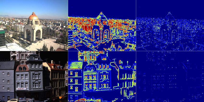
proach uses a pre-trained CNN for feature detection.               the detected keypoints are also evaluated on how ‘match-
   ELF computes the gradient of a trained CNN feature              able’ they are with the matching score [26]. This metric
map with respect to w.r.t the image: this outputs a saliency       requires to describe the keypoints so we define a simple
map with local maxima on keypoint positions. Trained               descriptor: it is based on the interpolation of a CNN fea-
detectors learn this saliency map with a CNN whereas we            ture map on the detected keypoints, as in [12]. This avoids
extract it with gradient computations. This approach is            biasing the performance by choosing an existing compet-
inspired by [35] which observes that the gradient of clas-         itive descriptor. Experiments show that even this simple
sification scores w.r.t the image is similar to the image          descriptor reaches competitive results which comforts the
saliency map. ELF differs in that it takes the gradient of         observation of [13], on the relevance of CNN features as
feature maps and not the classification score contrary to          descriptors. More details are provided section 4.1.
existing work exploiting CNN gradients [33, 37, 38, 40].              ELF is tested on five architectures: three classification
These previous works aim at visualising the learning sig-          networks trained on ImageNet classification: AlexNet,
nal for classification specifically whereas ELF extracts           VGG and Xception [9, 18, 36], as well as SuperPoint [12]
the feature locations. The extracted saliency map is then          and LF-Net [28] descriptor networks. Although outside
thresholded to keep only the most relevant locations and           the scope of this paper, this comparison provides prelim-
standard Non-Maxima Suppression (NMS) extracts the fi-             inary results of the influence of the network architecture,
nal keypoints (Figure 2).                                          task and training data on ELF’s performance. Metrics are
                                                                   computed on HPatches [5] for generic performances. We
                                                                   derive two auxiliary datasets from HPatches to study scale
                                                                   and rotation robustness. Light and 3D viewpoint robust-
                                                                   ness analysis are run on the Strecha, Webcam and datasets
                                                                   [39, 43]. These extensive experiments show that ELF is
                                                                   on par with other sparse detectors, which suggests that the
                                                                   feature representation and location information learnt by
                                                                   a CNN to complete a vision task is as relevant as when the
                                                                   CNN is specifically trained for feature detection. We addi-
                                                                   tionally test ELF’s robustness on 3D reconstruction from
                                                                   images in the context of the CVPR 2019 Image Match-
                                                                   ing challenge [1]. Once again, ELF is on par with other
                                                                   sparse methods even though denser methods, e.g. [12],
                                                                   are more appropriate for such a task. Our contributions
                                                                   are the following:
                                                                     • We show that a CNN trained on a standard vision
Figure 2: Saliency maps thresholding to keep only the                  task embeds feature location in the feature gradients.
most informative location. Top: original image. (Left-                 This information is as relevant for feature detection
Right: Webcam [43], HPatches [5], COCO[20]) Middle:                    as when a CNN is specifically trained for it.
blurred saliency maps. Bottom: saliency map after thresh-
old. (Better seen on a computer.)                                    • We define a systematic method for local feature de-
                                                                       tection. Extensive experiments show that ELF is on
   ELF relies only on six parameters: 2×2 Gaussian blur                par with other SoA deep trained detectors. They
parameters for the automatic threshold level estimation                also update the previous result from [13]: self-taught
and for the saliency map denoising; and two parameters                 CNN features provide SoA descriptors in spite of re-
for the (NMS) window and the border to ignore. Detec-                  cent improvements in CNN descriptors [10].
tion only requires one forward and one backward passes        • We release the python-based evaluation code to ease
and takes ∼0.2s per image on a simple Quadro M2200,              future comparison together with ELF code1 . The in-
which makes it suitable for real-time applications.              troduced robustness datasets are also made public 2 .
   ELF is compared to individual detectors with standard
repeatability [26] but results show that this metric is not
discriminative enough. Most of the existing detectors can 2 Related work
extract keypoints repeated across images with similar re-
peatability scores. Also, this metric does not express how Early methods rely on hand-crafted detection and descrip-
‘useful’ the detected keypoints are: if we sample all pix- tion : SIFT [21] detects 3D spatial-scale keypoints on dif-
els as keypoints, we reach 100% of rep. but the matching      1 ELF code:https://github.com/ELF-det/elf

may not be perfect if many areas look alike. Therefore,       2 Rotation and scale dataset: https://bit.ly/31RAh1S

                                                               2
ference of gaussians and describes them with a 3D His-             jective camera model to project detected keypoints from
togram Of Gradients (HOG). SURF [7] uses image inte-               one image to the other. These keypoint pairs form the
gral to speed up the previous detection and uses a sum             ground-truth matching points to train the network. ELF
of Haar wavelet responses for description. KAZE [4]                differs in that the CNN model is already trained on a stan-
extends the previous multi-scale approach by detecting             dard task. It then extracts the relevant information embed-
features in non-linear scale spaces instead of the classic         ded inside the network for local feature detection, which
Gaussian ones. ORB [30] combines the FAST [29] de-                 requires no training nor supervision.
tection, the BRIEF [8] description, and improves them to              The detection method of this paper is mainly inspired
make the pipeline scale and rotation invariant. MSER-              from the initial observation in [35]: given a CNN trained
based detector hand-crafts desired invariance properties           for classification, the gradient of a class score w.r.t the im-
for keypoints, and designs a fast algorithm to detect              age is the saliency map of the class object in the input
them [23]. Even though these hand-crafted methods have             image. A line of works aims at visualizing the CNN rep-
proven to be successful and to reach state-of-the-art per-         resentation by inverting it into the image space through
formance for some applications, recent research focus on           optimization [14, 22]. Our work differs in that we back-
learning-based methods.                                            propagate the feature map itself and not a feature loss.
   One of the first learned detector is TILDE [43], trained        Following works use these saliency maps to better un-
under drastic changes of light and weather on the We-              derstand the CNN training process and justify the CNN
bcam dataset. They use supervision to learn saliency               outputs. Efforts mostly focus on the gradient definitions
maps which maxima are keypoint locations. Ground-truth             [37, 38, 40, 46]. They differ in the way they handle
saliency maps are generated with ‘good keypoints’: they            the backpropagation of the non-linear units such as Relu.
use SIFT and filter out keypoints that are not repeated in         Grad-CAM [33] introduces a variant where they fuse sev-
more than 100 images. One drawback of this method is               eral gradients of the classification score w.r.t feature maps
the need for supervision that relies on another detector.          and not the image space. Instead, ELF computes the gra-
However, there is no universal explicit definition of what a       dient of the feature map, and not a classification score,
good keypoint is. This lack of specification inspires Quad-        w.r.t the image. Also we run simple backpropagation
Networks [31] to adopt an unsupervised approach: they              which differs in the non-linearity handling: all the sig-
train a neural network to rank keypoints according to their        nal is backpropagated no matter whether the feature maps
robustness to random hand-crafted transformations. They            or the gradients are positive or not. Finally, as far as we
keep the top/bottom quantile of the ranking as keypoints.          know, this is the first work to exploit the localisation in-
ELF is similar in that it does not requires supervision but        formation present in these gradients for feature detection.
differs in that it does not need to further train the CNN.            The simple descriptor introduced for the sake of the
   Other learned detectors are trained within full detec-          matchability evaluation is taken from UCN [10]. Given
tion/description pipelines such as LIFT [44], SuperPoint           a feature map and the keypoints to describe, it interpo-
[12] and LF-Net [28]. LIFT contribution lies in their orig-        lates the feature map on the keypoints location. Using
inal training method of three CNNs. The detector CNN               a trained CNN for feature description is one of the early
learns a saliency map where the most salient points are            applications of CNN [13]. Later, research has taken on
keypoints. They then crop patches around these key-                specifically training the CNN to generate features suit-
points, compute their orientations and descriptors with            able for keypoint matching either with patch-based ap-
two other CNNs. They first train the descriptor with               proaches, among which [15, 24, 34, 45], or image-based
patches around ground-truth matching points with con-              approaches [10, 41]. We choose the description method
trastive loss, then the orientation CNN together with the          from UCN [10], also used by SuperPoint, for its com-
descriptor and finally with the detector. One drawback of          plexity is only O(1) compared to patch-based approaches
this method is the need for ground-truth matching key-             that are O(N ) with N the number of keypoints. We favor
points to initiate the training. In [12], the problem is           UCN to InLoc [41] as it is simpler to compute. The moti-
avoided by pre-training the detector on a synthetic ge-            vation here is only to get a simple descriptor easy to inte-
ometric dataset made of polygons on which they detect              grate with all detectors for fair comparison of the detector
mostly corners. The detector is then finetuned during              matching performances. So we overlook the description
the descriptor training on image pairs from COCO [20]              performance.
with synthetic homographies and the correspondence con-
trastive loss introduced in [10]. LF-Net relies on another
type of supervision: it uses ground-truth camera poses and         3    Method
image depth maps that are easier to compute with laser or
standard SfM than ground-truth matching keypoints. Its             This section defines ELF, a detection method valid for any
training pipeline builds over LIFT and employs the pro-            trained CNN. Keypoints are local maxima of a saliency

                                                               3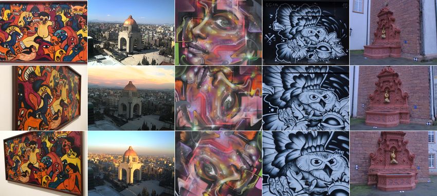
map computed as the feature gradient w.r.t the image. We 3.2 Feature Map Selection
use the data adaptive Kapur method [17] to automatically
threshold the saliency map and keep only the most salient We provide    visual guidelines to choose the feature level l
                                                                    l
locations, then run NMS for local maxima detection.       so that F   still holds high resolution localisation informa-
                                                          tion while providing a useful high-level representation.
                                                             CNN operations such as convolution and pooling in-
                                                          crease the receptive field of feature maps while reducing
                                                          their spatial dimensions. This means that F l has less spa-
                                                          tial resolution than F l−1 and the backpropagated signal
                                                          S l ends up more spread than S l−1 . This is similar to
                                                          when an image is too enlarged and it can be observed
                                                          in Figure 3, which shows the gradients of the VGG fea-
                                                          ture maps. On the top row, pool2 ’s gradient (left) better
                                                          captures the location details of the dome whereas pool3 ’s
                                                          gradient (right) is more spread. On the bottom rows, the
                                                          images lose their resolution as we go higher in the net-
                                                          work. Another consequence of this resolution loss is that
                                                          small features are not embedded in F l if l is too high.
                                                          This would reduce the space of potential keypoint to only
                                                          large features which would hinder the method. This ob-
                                                          servation motivates us to favor low-level feature maps for
                                                          feature detection. We chose the final F l by taking the
                                                          highest l which provides accurate localisation. This is vi-
                                                          sually observable by sparse high intensity signal contrary
Figure 3: (Bigger version Figure 15.) Saliency maps com- to the blurry aspect of higher layers.
                                                    l
puted from the feature map gradient T F l (x) · ∂F
                                                 ∂I . En-
hanced image contrast for better visualisation. Top row:           3.3    Automatic Data-Adaptive Thresholding
gradients of VGG pool2 and pool3 show a loss of reso-
                                                                   The threshold is automatic and adapts to the saliency map
lution from pool2 to pool3 . Bottom: (pooli )i∈[1,2,5] of
                                                                   distribution to keep only the most informative regions.
VGG on Webcam, HPatches and Coco images. Low level
                                                                   Figure 2 shows saliency maps before and after threshold-
saliency maps activate accurately whereas higher saliency
                                                                   ing using Kapur’s method [17], which we briefly recall
maps are blurred.
                                                                   below. It chooses the threshold to maximize the infor-
                                                                   mation between the image background and foreground
                                                                   i.e. the pixel distribution below and above the thresh-
3.1    Feature Specific Saliency                                   old. This method is especially relevant in this case as it
                                                                   aims at maintaining as much information on the distribu-
We generate a saliency map that activates on the most in-
                                                                   tion above the threshold as possible. This distribution de-
formative image region for a specific CNN feature level l.
                                                                   scribes the set of local maxima among which we choose
Let I be a vector image of dimension DI = HI · WI · CI .
                                                                   our keypoints. More formally, for an image I of N pix-
Let F l be a vectorized feature map of dimension DF =
                                                                   els with n sorted gray levels and (fi )i∈n the correspond-
Hl · Wl · Cl . The saliency map S l , of dimension DI , is                                fi
                                                                   ing histogram, pi = N     is the empirical probability of a
S l (I) = t F l (I) · ∇I F l , with ∇I F l a DF × DI matrix.
                                                                   pixel to hold the value fi . Let s ∈ n be a threshold level
    The saliency activates on the image regions that con-
                                                                   and A, B the empirical background and foreground distri-
tribute the most to the feature representation F l (I). The
                                                                   butions. The level s is chosen to maximize the informa-
term ∇I F l explicits the correlation between the feature
space of F l and the image space in general. The multi-
                                                                   tion between
                                                                                 Aand B and the threshold
                                                                                                               is set to fs :
                                                                                                             value
                                                                              pi                        pi
plication by F l (I) applies the correlation to the features       A=      P
                                                                                 pi     and B =      P
                                                                                                            pi     . For better
                                                                            is
F l (I) specifically and generate a visualisation in image         results, we blur the image with a Gaussian of parameters
space S l (I). From a geometrical point of view, this oper-        (µthr , σthr ) before computing the threshold level.
ation can be seen as the projection ∇I F l of a feature sig-          Once the threshold is set, we denoise the image with a
nal F l (I) into the image space. From a signal processing         second Gaussian blur of parameters (µnoise , σnoise ) and
approach, F l (I) is an input signal filtered through ∇I F l       run standard NMS (the same as for SuperPoint) where we
into the image space. If CI > 1, S l is converted into a           iteratively select decreasing global maxima while ensur-
grayscale image by averaging it across channels.                   ing that their nearest neighbor distance is higher than the

                                                               4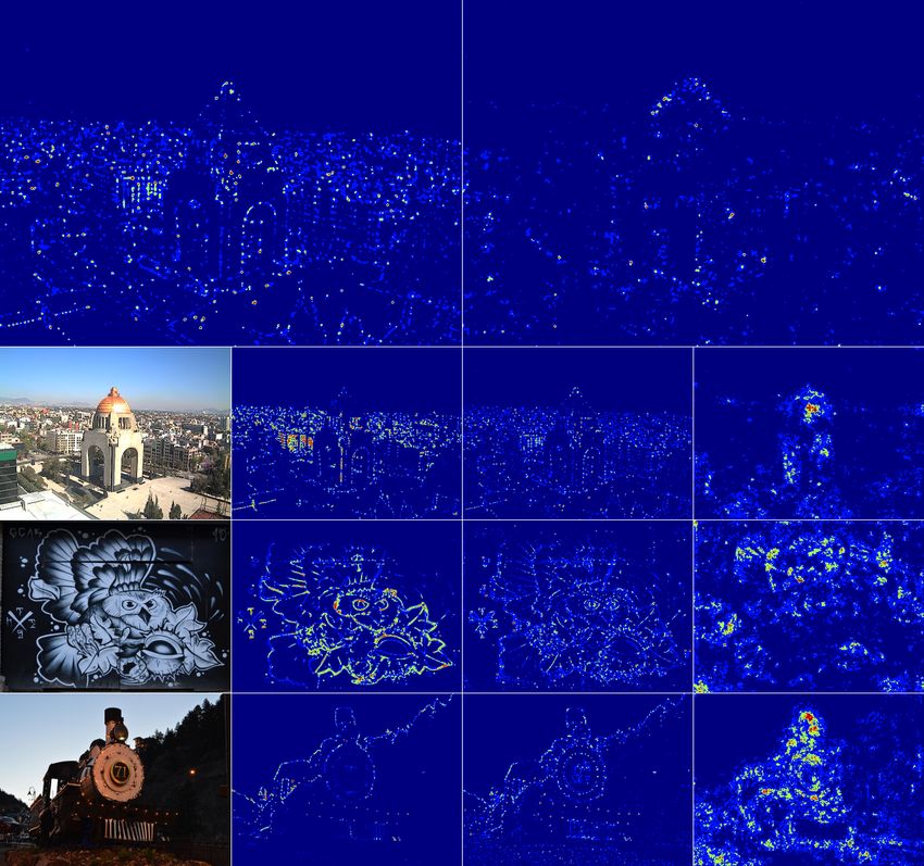
window wNMS ∈ N. Also we ignore the bNMS ∈ N pixels crafted SIFT [21], SURF [7], ORB [30], KAZE [4], the
around the image border.                            learning-based LIFT [44], SuperPoint [12], LF-Net [28],
                                                    the individual detectors TILDE [43], MSER [23].
3.4    Simple descriptor
                                                                     4.1    Metrics
As mentioned in the introduction, the repeatability score
does not discriminate among detectors anymore. So they               We follow the standard validation guidelines [26] that
are also evaluated on how ‘matchable’ their detected key-            evaluates the detection performance with repeatability
points are with the matching score. To do so, the ELF                (rep). It measures the percentage of keypoints common to
detector is completed with a simple descriptor inspired by           both images. We also compute the matching score (ms) as
SuperPoint’s descriptor. The use of this simple descrip-             an additional detector metric. It captures the percentage
tor over existing competitive ones avoids unfairly boost-            of keypoint pairs that are nearest neighbours in both im-
ing ELF’s perfomance. Inspired by SuperPoint, we in-                 age space and descriptor space i.e. the ratio of keypoints
terpolate a CNN feature map on the detected keypoints.               correctly matched. For fair completeness, the mathemat-
Although simple, experiments show that this simple de-               ical definitions of the metrics are provided in Appendix
scriptor completes ELF into a competitive feature detec-             and their implementation in the soon-to-be released code.
tion/description method.                                                A way to reach perfect rep is to sample all the pixels
   The feature map used for description may be different             or sample them with a frequency higher than the distance
from the one for detection. High-level feature maps have             threshold kp of the metric. One way to prevent the first
wider receptive field hence take higher context into ac-             flaw is to limit the number of keypoints but it does not
count for the description of a pixel location. This leads            counter the second. Since detectors are always used to-
to more informative descriptors which motivates us to fa-            gether with descriptors, another way to think the detector
vor higher level maps. However we are also constrained               evaluation is: ’a good keypoint is one that can be discrim-
by the loss of resolution previously described: if the fea-          inatively described and matched’. One could think that
ture map level is too high, the interpolation of the descrip-        such a metric can be corrupted by the descriptor. But we
tors generate vector too similar to each other. For exam-            ensure that a detector flaw cannot be hidden by a very
ple, the VGG pool4 layer produces more discriminative                performing descriptor with two guidelines. One experi-
descriptors than pool5 even though pool5 embeds infor-               ment must evaluate all detector with one fixed descriptor
mation more relevant for classification. Empirically we              (the simple one defined in 3.4). Second, ms can never be
observe that there exists a layer level l0 above which the           higher than rep so a detector with a poor rep leads to a
description performance stops increasing before decreas-             poor ms.
ing. This is measured through the matching score metric                 Here the number of detected keypoints is limited to 500
introduced in [26]. The final choice of the feature map is           for all methods. As done in [12, 28], we replace the over-
done by testing some layers l0 > l and select the lowest             lap score in [26] to compute correspondences with the 5-
feature map before the descriptor performance stagnates.             pixel distance threshold. Following [44], we also mod-
   The compared detectors are evaluated with both their              ify the matching score definition of [26] to run a greedy
original descriptor and this simple one. We detail the mo-           bipartite-graph matching on all descriptors and not just
tivation behind this choice: detectors may be biased to              the descriptor pairs for which the distance is below an ar-
sample keypoints that their respective descriptor can de-            bitrary threshold. We do so to be able to compare all state-
scribe ‘well’ [44]. So it is fair to compute the matching            of-the-art methods even when their descriptor dimension
score with the original detector/descriptor pairs. How-              and range vary significantly. (More details in Appendix.)
ever, a detector can sample ‘useless points’ (e.g. sky pix-
els for 3d reconstructions) that its descriptor can charac-          4.2    Datasets
terise ‘well’. In this case, the descriptor ‘hides’ the detec-
tor default. This motivates the integration of a common    All images are resized to the 480×640 pixels and the im-
independent descriptor with all detectors to evaluate them.age pair transformations are rectified accordingly.
Both approaches are run since each is as fair as the other.  General performances. The HPatches dataset [5]
                                                           gathers a subset of standard evaluation images such as
                                                           DTU and OxfordAffine [2, 25]: it provides a total of 696
4 Experiments                                              images, 6 images for 116 scenes and the corresponding
                                                           homographies between the images of a same scene. For
This section describes the evaluation metrics and datasets 57 of these scenes, the main changes are photogrammetric
as well as the method’s tuning. Our method is compared and the remaining 59 show significant geometric deforma-
to detectors with available public code: the fully hand- tions due to viewpoint changes on planar scenes.

                                                                 5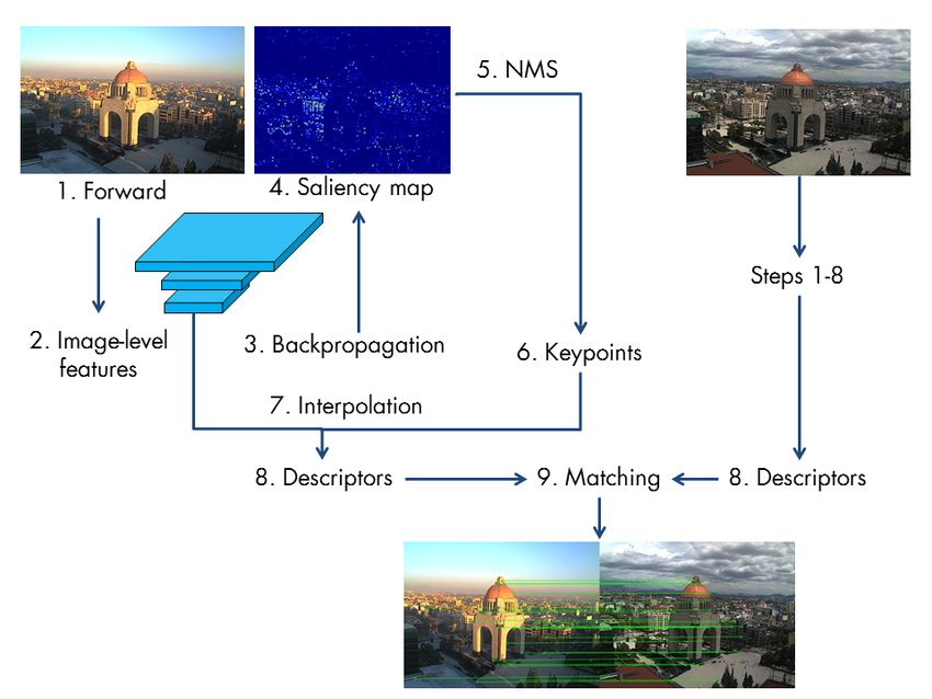
ELF as in saliency. The paper compares the influence
                                                                   of i) architecture for a fixed task (ELF-AlexNet [18] vs.
                                                                   ELF-VGG [36] v.s. ELF-Xception [9]), ii) the task (ELF-
                                                                   VGG vs. ELF-SuperPoint (SP) descriptor), iii) the train-
                                                                   ing dataset (ELF-LFNet on phototourism vs. ELF-SP on
                                                                   MS-COCO). This study is being refined with more inde-
                                                                   pendent comparisons of tasks, datasets and architectures
                                                                   soon available in a journal extension.
                                                                      We use the author’s code and pre-trained models
                                                                   which we convert to Tensorflow [3] except for LF-
Figure 4: Left-Right: HPatches: planar viewpoint. Web-
                                                                   Net. We search the blurring parameters (µthr , σthr ),
cam: light. HPatches: rotation. HPatches: scale. Strecha:
                                                                   (µnoise , σnoise ) in the range [[3, 21]]2 and the NMS pa-
3D viewpoint.
                                                                   rameters (wN M S , bN M S ) in [[4, 13]]2 .
                                                                      Individual components comparison. Individual de-
   Illumination Robustness. The Webcam dataset [43]                tectors are compared with the matchability of their de-
gathers static outdoor scenes with drastic natural light           tection and the description of the simple VGG-pool3 de-
changes contrary to HPatches which mostly holds artifi-            scriptor. This way, the m.s. only depends on the detec-
cial light changes in indoor scenes.                               tion performance since the description is fixed for all de-
   Rotation and Scale Robustness. We derive two                    tectors. The comparison between ELF and recent deep
datasets from HPatches. For each of the 116 scenes, we             methods raises the question of whether triplet-like losses
keep the first image and rotate it with angles from 0◦ to          are relevant to train CNN descriptors. Indeed, these losses
210◦ with an interval of 40◦ . Four zoomed-in version              constrain the CNN features directly so that matching key-
of the image are generated with scales [1.25, 1.5, 1.75, 2].       points are near each other in descriptor space. Simpler
We release these two datasets together with their ground           loss, such as cross-entropy for classification, only the con-
truth homographies for future comparisons.                         strain the CNN output on the task while leaving the repre-
   3D Viewpoint Robustness. We use three Strecha                   sentation up to the CNN.
scenes [39] with increasing viewpoint changes: Fountain,              ELF-VGG detector is also integrated with existing de-
Castle entry, Herzjesu-P8. The viewpoint changes pro-              scriptors. This evaluates how useful the CNN self-learned
posed by HPatches are limited to planar scenes which               feature localisation compares with the hand-crafted and
does not reflect the complexity of 3D structures. Since            the learned ones.
the ground-truth depths are not available anymore, we                 Gradient Baseline. Visually, the feature gradient map
use COLMAP [32] 3D reconstruction to obtain ground-                is reminiscent of the image gradients computed with the
truth scaleless depth. We release the obtained depth maps          Sobel or Laplacian operators. We run two variants of our
and camera poses together with the evaluation code. ELF            pipeline where we replace the feature gradient with them.
robustness is additionally tested in the CVPR19 Image              This aims at showing whether CNN feature gradients em-
Matching Challenge [1] (see results sections).                     bed more information than image intensity gradients.

4.3    Baselines
                                                                   5    Results
We describe the rationale behind the evaluation. The
tests run on a QuadroM2200 with Tensorflow 1.4, Cuda8,             Experiments show that ELF compares with the state-
Cudnn6 and Opencv3.4. We use the OpenCV implemen-                  of-the-art on HPatches and demonstrates similar robust-
tation of SIFT, SURF, ORB, KAZE, MSER with the de-                 ness properties with recent learned methods. It generates
fault parameters and the author’s code for TILDE, LIFT,            saliency maps visually akin to a Laplacian on very struc-
SuperPoint, LF-Net with the provided models and param-             tured images (HPatches) but proves to be more robust on
eters. When comparing detectors in the feature matching            outdoor scenes with natural conditions (Webcam). When
pipeline, we measure their matching score with both their          integrated with existing feature descriptors, ELF boosts
original descriptor and ELF simple descriptor. For MSER            the matching score. Even integrating ELF simple descrip-
and TILDE, we use the VGG simple descriptor.                       tor improves it with the exception of SuperPoint for which
   Architecture influence. ELF is tested on five net-              results are equivalent. This sheds new light on the repre-
works: three classification ones trained on ImageNet               sentations learnt by CNNs and suggests that deep descrip-
(AlexNet, VGG, Xception [9, 18, 36]) as well as the                tion methods may underexploit the information embed-
trained SuperPoint’s and LF-Net’s descriptor ones. We              ded in their trained networks. Another suggestion may
call each variant with the network’s names prefixed with           be that the current metrics are not relevant anymore for

                                                               6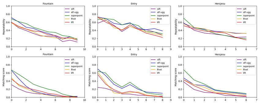
deep learning methods. Indeed, all can detect repeatable            door or outdoor datasets, whereas HPatches is made of a
keypoints with more or less the same performances. Even             mix of them. We compute metrics for both LF-Net models
though the matchability of the points (m.s) is a bit more           and report the highest one (indoor). Even though LF-Net
discriminative, neither express how ‘useful’ the kp are for         and LIFT fall behind the top learned methods, they still
the end-goal task. One way to do so is to evaluate an end-          outperform hand-crafted ones which suggests that their
goal task (e.g. Structure-from-Motion). However, for the            framework learn feature specific information that hand-
evaluation to be rigorous all the other steps should be fixed       crafted methods can not capture. This supports the recent
for all papers. Recently, the Image Matching CVPR19                 direction towards trained detectors and descriptors.
workshop proposed such an evaluation but is not fully au-              Light Robustness Again, ms is a better discriminant on
tomatic yet. These results also challenge whether current           Webcam than rep (Figure 5 bottom). ELF-VGG reaches
descriptor-training loss are a strong enough signal to con-         top rep-ms [53.2, 43.7] closely followed by TILDE [52.5,
strain CNN features better than a simple cross-entropy.             34.7] which was the state-of-the-art detector.
                                                                       Overall, there is a performance degradation (∼20%)
                                                                    from HPatches to Webcam. HPatches holds images
                                                                    with standard features such as corners that state-of-the-
                                                                    art methods are made to recognise either by definition or
                                                                    by supervision. There are less such features in the We-
                                                                    bcam dataset because of the natural lighting that blurs
                                                                    them. Also there are strong intensity variations that these
                                                                    models do not handle well. One reason may be that the
                                                                    learning-based methods never saw such lighting varia-
                                                                    tions in their training set. But this assumption is rejected
                                                                    as we observe that even SuperPoint, which is trained on
                                                                    Coco images, outperforms LIFT and LF-Net, which are
                                                                    trained on outdoor images. Another justification can be
                                                                    that what matters the most is the pixel distribution the net-
                                                                    work is trained on, rather than the image content. The top
                                                                    methods are classifier-based ELF and SuperPoint: the first
                                                                    ones are trained on the huge Imagenet dataset and benefit
                                                                    from heavy data augmentation. SuperPoint also employs
Figure 5: Top-Down: HPatches-Webcam. Left-Right: re-                a considerable data strategy to train their network. Thus
peatability, matching score.                                        these networks may cover a much wider pixel distribution
                                                                    which would explain their robustness to pixel distribution
   The tabular version of the following results is provided         changes such as light modifications.
in Appendix. The graph results are better seen with color              Architecture influence ELF is tested on three classifi-
on a computer screen. Unless mentioned otherwise, we                cation networks as well as the descriptor networks of Su-
compute repeatability for each detector, and the match-             perPoint and LF-Net (Figure 5, bars under ‘ELF’).
ing score of detectors with their respective descriptors,              For a fixed training task (classification) on a fixed
when they have one. We use ELF-VGG-pool4 descrip-                   dataset (ImageNet), VGG, AlexNet and Xception are
tor for TILDE, MSER, ELF-VGG, ELF-SuperPoint, and                   compared. As could be expected, the network architec-
ELF-LFNet. We use AlexNet and Xception feature maps                 ture has a critical impact on the detection and ELF-VGG
to build their respective simple descriptors. The meta-             outperforms the other variants. The rep gap can be ex-
parameters for each variants are provided in Appendix.              plained by the fact that AlexNet is made of wider convo-
   General performances. Figure 5 (top) shows that the              lutions than VGG, which induces a higher loss of resolu-
rep variance is low across detectors whereas ms is more             tion when computing the gradient. As for ms, the higher
discriminative, hence the validation method (Section 4.1).          representation space of VGG may help building more in-
On HPatches, SuperPoint (SP) reaches the best rep-ms                formative features which are a stronger signal to back-
[68.6, 57.1] closely followed by ELF (e.g. ELF-VGG:                 propagate. This could also justify why ELF-VGG out-
[63.8, 51.8]) and TILDE [66.0, 46.7]. In general, we ob-            performs ELF-Xception that has less parameters. An-
serve that learning-based methods all outperform hand-              other explanation is that ELF-Xception’s gradient maps
crafted ones. Still, LF-Net and LIFT curiously underper-            seem smoother. Salient locations are then less emphasized
form on HPatches: one reason may be that the data they              which makes the keypoint detection harder. One could
are trained on differs too much from this one. LIFT is              hint at the depth-wise convolution to explain this visual
trained on outdoor images only and LF-Net on either in-             aspect but we could not find an experimental way to verify

                                                                7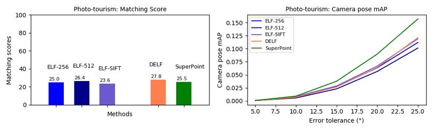
it. Surprisingly, ELF-LFNet outperforms the original LF- These results suggest that the orientation learning step in
Net on both HPatches and Webcam and ELF-SuperPoint LIFT and LF-Net is needed but its robustness could be
variant reaches similar results as the original.         improved.

     Figure 6: HPatches scale. Left-Right: rep, ms.
                                                                         Figure 8: Robustness analysis: 3D viewpoint.
   Scale Robustness. ELF-VGG is compared with state-
                                                                      3D Viewpoint Robustness. While SIFT shows a clear
of-the art detectors and their respective descriptors (Fig-
                                                                   advantage of pure-rotation robustness, it displays simi-
ure 6). Repeatability is mostly stable for all methods:
                                                                   lar degradation as other methods on realistic rotation-and-
SIFT and SuperPoint are the most invariant whereas ELF
                                                                   translation on 3D structures. Figure 8 shows that all meth-
follows the same variations as LIFT and LF-Net. Once
                                                                   ods degrade uniformly. One could assume that this small
again, ms better assesses the detectors performance: Su-
                                                                   data sample is not representative enough to run such ro-
perPoint is the most robust to scale changes, followed by
                                                                   bustness analysis. However, we think that these results
LIFT and SIFT. ELF and LF-Net lose 50% of their match-
                                                                   rather suggest that all methods have the same robustness
ing score with the increasing scale. It is surprising to ob-
                                                                   to 3D viewpoint changes. Even though previous analyses
serve that LIFT is more scale-robust than LF-Net when
                                                                   allows to rank the different feature matching pipelines,
the latter’s global performance is higher. A reasonable ex-
                                                                   each has advantages over others on certain situations:
planation is that LIFT detects keypoints at 21 scales of the
                                                                   ELF or SuperPoint on general homography matches, or
same image whereas LF-Net only runs its detector CNN
                                                                   SIFT on rotation robustness. This is why this paper only
on 5 scales. Nonetheless, ELF outperforms LF-Net with-
                                                                   aims at showing ELF reaches the same performances and
out manual multi-scale processing.
                                                                   shares similar properties to existing methods as there is
                                                                   no generic ranking criteria. The recent evaluation run by
                                                                   the CVPR19 Image Matching Challenge [1] supports the
                                                                   previous conclusions.

    Figure 7: HPatches rotation. Left-Right: rep, ms.

   Rotation Robustness. Even though rep shows little               Figure 9: Left-Middle-Right bars: original method, inte-
variations (Figure 7), all learned methods’ ms crash while         gration of ELF detection, integration of ELF description.
only SIFT survives the rotation changes. This can be ex-
plained by the explicit rotation estimation step of SIFT.             Individual components performance. First, all meth-
However LIFT and LF-Net also run such a computation.               ods’ descriptor are replaced with the simple ELF-VGG-
This suggests that either SIFT’s hand-crafted orientation          pool3 one. We then compute their new ms and com-
estimation is more accurate or that HOG are more rota-             pare it to ELF-VGG on HPatches and Webcam (Figure
tion invariant than learned features. LF-Net still performs        9, stripes). The description is based on pool3 instead of
better than LIFT: this may be because it learns the key-           pool4 here for it produces better results for the other meth-
point orientation on the keypoint features representation          ods while preserving ours. ELF reaches higher ms [51.3]
rather than the keypoint pixels as done in LIFT. Not sur-          for all methods except for SuperPoint [53.7] for which
prisingly, ELF simple descriptor is not rotation invariant         it is comparable. This shows that ELF is as relevant, if
as the convolutions that make the CNN are not. This also           not more, than previous hand-crafted or learned detectors.
explains why SuperPoint also crashes in a similar manner.          This naturally leads to the question: ’What kind of key-

                                                               8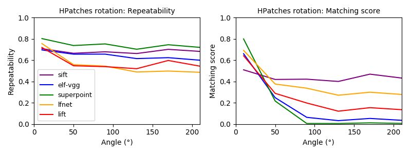
points does ELF detect ?’ There is currently no answer                completed with simple ELF descriptors from the VGG,
to this question as it is complex to explicitly characterize          AlexNet and Xception networks. These new hybrids are
properties of the pixel areas around keypoints. Hence the             then compared to their respective ELF variant (Right).
open question ’What makes a good keypoint ?’ mentioned                Results show that these simpler gradients can detect sys-
at the beginning of the paper. Still, we observe that ELF             tematic keypoints with comparable rep on very structured
activates mostly on high intensity gradient areas although            images such as HPatches. However, the ELF detector bet-
not all of them. One explanation is that as the CNN is                ter overcomes light changes (Webcam). On HPatches,
trained on the vision task, it learns to ignore image regions         the Laplacian-variant reaches similar ms as ELF-VGG (55
useless for the task. This results in killing the gradient sig-       vs 56) and outperforms ELF-AlexNet and ELF-Xception.
nals in areas that may be unsuited for matching.                      These scores can be explained with the images structure:
   Another surprising observation regards CNN descrip-                for heavy textured images, high intensity gradient loca-
tors: SuperPoint (SP) keypoints are described with the                tions are relevant enough keypoints. However, on Web-
SP descriptor in one hand and the simple ELF-VGG one                  cam, all ELF detectors outperform Laplacian and Sobel
in the other hand. Comparing the two resulting match-                 with a factor of 100%. This shows that ELF is more ro-
ing scores is one way to compare the SP and ELF de-                   bust than Laplacian and Sobel operators. Also, feature
scriptors. Results show that both approaches lead to sim-             gradient is a sparse signal which is better suited for lo-
ilar ms. This result is surprising because SP specifically            cal maxima detection than the much smoother Laplacian
trains a description CNN so that its feature map is suit-             operator (Figure 11).
able for keypoint description [10]. In VGG training, there
is no explicit constraints on the features from the cross-
entropy loss. Still, both feature maps reach similar nu-
merical description performance. This raises the question
of whether contrastive-like losses, which input are CNN
features, can better constrain the CNN representation than
simpler losses, such as cross-entropy, which inputs are
classification logits. This also shows that there is more
to CNNs than only the task they are trained on: they em-
bed information that can prove useful for unrelated tasks.            Figure 11: Feature gradient (right) provides a sparser sig-
Although the simple descriptor was defined for evaluation             nal than Laplacian (middle) which is more selective of
purposes, these results demonstrate that it can be used as            salient areas.
a description baseline for feature extraction.
   The integration of ELF detection with other methods’                 Qualitative results Green lines show putative matches
descriptor (Figure 9, circle) boosts the ms. [44] previously          based only on nearest neighbour matching of descriptors.
suggested that there may be a correlation between the de-             More qualitative results are available in the video 3 .
tector and the descriptor within a same method, i.e. the
LIFT descriptor is trained to describe only the keypoints
output by its detector. However, these results show that
ELF can easily be integrated into existing pipelines and
even boost their performances.                                        Figure 12: Green lines show putative matches of the sim-
                                                                      ple descriptor before RANSAC-based homography esti-
                                                                      mation.

                                                            CVPR19 Image Matching Challenge [1] This chal-
                                                         lenge evaluates detection/description methods on two
                                                         standard tasks: 1) wide stereo matching and 2) structure
                                                         from motion from small image sets. The matching score
                                                         evaluates the first task, and the camera pose estimation
                                                         is used for both tasks. Both applications are evaluated on
                                                         the photo-tourism image collections of popular landmarks
              Figure 10: Gradient baseline.              [16, 42]. More details on the metrics definition are avail-
                                                         able on the challenge website [1].
  Gradient Baseline The saliency map used in ELF is
                                                            Wide stereo matching: Task 1 matches image pairs
replaced with simple Sobel or Laplacian gradient maps.
                                                         across wide baselines. It is evaluated with the keypoints
The rest of the detection pipeline stays the same and we
compute their performance (Figure 10 Left). They are        3 https://youtu.be/oxbG5162yDs

                                                                  9
ms and the relative camera pose estimation between two
images. The evaluators run COLMAP to reconstruct
dense ‘ground-truth’ depth which they use to translate
keypoints from one image to another and compute the
matching score. They use the RANSAC inliers to estimate
the camera pose and measure performance with the “an-
gular difference between the estimated and ground-truth
vectors for both rotation and translation. To reduce this to
one value, they use a variable threshold to determine each
pose as correct or not, then compute the area under the Figure 14: SfM from small subsets. Evolution of mAP of
curve up to the angular threshold. This value is thus the camera pose for increasing tolerance threshold.
mean average precision up to x, or mAPx. They consider
5, 10, 15, 20, and 25 degrees” [1]. Submissions can con-
tain up to 8000 keypoints and we submitted entries to the
Structure-from-Motion from small subsets. Task 2 “pro-
sparse category i.e. methods with up to 512 keypoints.
poses to to build SfM reconstructions from small (3, 5, 10,
25) subsets of images and use the poses obtained from the
entire (much larger) set as ground truth” [1].
Figure 14 shows that SuperPoint reaches performance
twice as big as the next best method ELF-SIFT. This sug-
gests that when few images are available, SuperPoint per-
forms better than other approaches. One explanation is
that even in ’sparse-mode’, i.e. when the number of key-
Figure 13: Wide stereo matching. Left: matching score points is restricted up to 512, SuperPoint samples points
(%) of sparse methods (up to 512 keypoints) on photo- more densely than the others (∼383 v.s. ∼210 for the oth-
tourism. Right: Evolution of mAP of camera pose for ers). Thus, SuperPoint provides more keypoints to trian-
increasing tolerance threshold (degrees). gulate i.e. more 2D-3D correspondences to use when esti-
mating the camera pose. This suggests that high keypoint
Figure 13 (left) shows the ms (%) of the submitted density is a crucial characteristic of the detection method
sparse methods. It compares ELF-VGG detection with for Structure-from-Motion. In this regard, ELF still has
DELF [27] and SuperPoint, where ELF is completed with room for improvement compared to SuperPoint.
either the simple descriptor from pool3 or pool4, and
SIFT. The variant are dubbed respectively ELF-256, ELF-
512 and ELF-SIFT. This allows us to sketch a simple com-
parison of descriptor performances between the simple
descriptor and standard SIFT. 6 Conclusion
As previously observed on HPatches and Webcam, ELF
and SuperPoint reach similar scores on Photo-Tourism. We have introduced ELF, a novel method to extract fea-
ELF-performance slightly increases from 25% to 26.4% ture locations from pre-trained CNNs, with no further
when switching descriptors from VGG-pool3 to VGG- training. Extensive experiments show that it performs
pool4. One explanation is that the feature space size is as well as state-of-the art detectors. It can easily be in-
doubled from the first to the second. This would allow the tegrated into existing matching pipelines and proves to
pool4 descriptors to be more discriminative. However, the boost their matching performances. Even when com-
1.4% gain may not be worth the additional memory use. pleted with a simple feature-map-based descriptor, it turns
Overall, the results show that ELF can compare with the into a competitive feature matching pipeline. These re-
SoA on this additional dataset that exhibits more illumina- sults shed new light on the information embedded inside
tion and viewpoint changes than HPatches and Webcam. trained CNNs. This work also raises questions on the
This observation is reinforced by the camera pose eval- descriptor training of deep-learning approaches: whether
uation (Figure 13 right). SuperPoint shows as slight ad- their losses actually constrain the CNN to learn better fea-
vantage over others that increases from 1% to 5% across tures than the ones it would learn on its own to complete a
the error tolerance threshold whereas ELF-256 exhibits a vision task. Preliminary results show that the CNN archi-
minor under-performance. Still, these results show ELF tecture, the training task and the dataset have substantial
compares with SoA performance even though it is not impact on the detector performances. A further analysis
trained explicitly for detection/description. of these correlations is the object of a future work.
10References [14] G ATYS , L. A., E CKER , A. S., AND B ETHGE , M. Image
style transfer using convolutional neural networks. In Pro-
[1] Cvpr19 image matching challenge. https: ceedings of the IEEE Conference on Computer Vision and
//image-matching-workshop.github.io/ Pattern Recognition (2016), pp. 2414–2423.
challenge/, 2019.
[15] H AN , X., L EUNG , T., J IA , Y., S UKTHANKAR , R., AND
[2] A ANÆS , H., DAHL , A. L., AND P EDERSEN , K. S. Inter- B ERG , A. C. Matchnet: Unifying feature and metric learn-
esting interest points. International Journal of Computer ing for patch-based matching. In Proceedings of the IEEE
Vision 97, 1 (2012), 18–35. Conference on Computer Vision and Pattern Recognition
[3] A BADI , M., BARHAM , P., C HEN , J., C HEN , Z., DAVIS , (2015), pp. 3279–3286.
A., D EAN , J., D EVIN , M., G HEMAWAT, S., I RVING , G.,
I SARD , M., ET AL . Tensorflow: a system for large-scale [16] H EINLY, J., S CHONBERGER , J. L., D UNN , E., AND
machine learning. In OSDI (2016), vol. 16, pp. 265–283. F RAHM , J.-M. Reconstructing the world* in six days*(as
captured by the yahoo 100 million image dataset). In Pro-
[4] A LCANTARILLA , P. F., BARTOLI , A., AND DAVISON , ceedings of the IEEE Conference on Computer Vision and
A. J. Kaze features. In European Conference on Com- Pattern Recognition (2015), pp. 3287–3295.
puter Vision (2012), Springer, pp. 214–227.
[17] K APUR , J. N., S AHOO , P. K., AND W ONG , A. K. A
[5] BALNTAS , V., L ENC , K., V EDALDI , A., AND M IKO - new method for gray-level picture thresholding using the
LAJCZYK , K. Hpatches: A benchmark and evaluation entropy of the histogram. Computer vision, graphics, and
of handcrafted and learned local descriptors. In Confer- image processing 29, 3 (1985), 273–285.
ence on Computer Vision and Pattern Recognition (CVPR)
(2017), vol. 4, p. 6. [18] K RIZHEVSKY, A., S UTSKEVER , I., AND H INTON , G. E.
Imagenet classification with deep convolutional neural net-
[6] BALNTAS , V., R IBA , E., P ONSA , D., AND M IKOLA - works. In Advances in neural information processing sys-
JCZYK , K. Learning local feature descriptors with triplets
tems (2012), pp. 1097–1105.
and shallowconvolutional neural networks. In BMVC
(2016), vol. 1, p. 3. [19] L ENC , K., G ULSHAN , V., AND V EDALDI , A.
[7] BAY, H., T UYTELAARS , T., AND VAN G OOL , L. Surf: Vlbenchmkars. http://www.vlfeat.org/
Speeded up robust features. In European conference on benchmarks/xsxs, 2011.
computer vision (2006), Springer, pp. 404–417.
[20] L IN , T.-Y., M AIRE , M., B ELONGIE , S., H AYS , J., P ER -
[8] C ALONDER , M., L EPETIT, V., S TRECHA , C., AND F UA , ONA , P., R AMANAN , D., D OLL ÁR , P., AND Z ITNICK ,
P. Brief: Binary robust independent elementary fea- C. L. Microsoft coco: Common objects in context. In
tures. In European conference on computer vision (2010), European conference on computer vision (2014), Springer,
Springer, pp. 778–792. pp. 740–755.
[9] C HOLLET, F. Xception: Deep learning with depthwise [21] L OWE , D. G. Distinctive image features from scale-
separable convolutions. In 2017 IEEE Conference on Com- invariant keypoints. International journal of computer vi-
puter Vision and Pattern Recognition, CVPR 2017, Hon- sion 60, 2 (2004), 91–110.
olulu, HI, USA, July 21-26, 2017 (2017), pp. 1800–1807.
[22] M AHENDRAN , A., AND V EDALDI , A. Understanding
[10] C HOY, C. B., G WAK , J., S AVARESE , S., AND C HAN - deep image representations by inverting them. In Proceed-
DRAKER , M. Universal correspondence network. In Ad- ings of the IEEE conference on computer vision and pat-
vances in Neural Information Processing Systems (2016), tern recognition (2015), pp. 5188–5196.
pp. 2414–2422.
[23] M ATAS , J., C HUM , O., U RBAN , M., AND PAJDLA , T.
[11] D ENG , J., D ONG , W., S OCHER , R., L I , L.-J., L I , K.,
Robust wide-baseline stereo from maximally stable ex-
AND F EI -F EI , L. Imagenet: A large-scale hierarchical im-
tremal regions. Image and vision computing 22, 10 (2004),
age database. In Computer Vision and Pattern Recogni-
761–767.
tion, 2009. CVPR 2009. IEEE Conference on (2009), Ieee,
pp. 248–255.
[24] M ELEKHOV, I., K ANNALA , J., AND R AHTU , E. Siamese
[12] D E T ONE , D., M ALISIEWICZ , T., AND R ABINOVICH , A. network features for image matching. In 2016 23rd In-
Superpoint: Self-supervised interest point detection and ternational Conference on Pattern Recognition (ICPR)
description. In CVPR Deep Learning for Visual SLAM (2016), IEEE, pp. 378–383.
Workshop (2018).
[25] M IKOLAJCZYK , K., AND S CHMID , C. A performance
[13] F ISCHER , P., D OSOVITSKIY, A., AND B ROX , T. Descrip- evaluation of local descriptors. IEEE transactions on
tor matching with convolutional neural networks: a com- pattern analysis and machine intelligence 27, 10 (2005),
parison to sift. arXiv preprint arXiv:1405.5769 (2014). 1615–1630.
11[26] M IKOLAJCZYK , K., T UYTELAARS , T., S CHMID , C., [39] S TRECHA , C., VON H ANSEN , W., VAN G OOL , L., F UA ,
Z ISSERMAN , A., M ATAS , J., S CHAFFALITZKY, F., P., AND T HOENNESSEN , U. On benchmarking camera
K ADIR , T., AND VAN G OOL , L. A comparison of affine calibration and multi-view stereo for high resolution im-
region detectors. International journal of computer vision agery. In Computer Vision and Pattern Recognition, 2008.
65, 1-2 (2005), 43–72. CVPR 2008. IEEE Conference on (2008), Ieee, pp. 1–8.
[27] N OH , H., A RAUJO , A., S IM , J., W EYAND , T., AND [40] S UNDARARAJAN , M., TALY, A., AND YAN , Q. Ax-
H AN , B. Largescale image retrieval with attentive deep iomatic attribution for deep networks. In International
local features. In Proceedings of the IEEE International Conference on Machine Learning (2017), pp. 3319–3328.
Conference on Computer Vision (2017), pp. 3456–3465.
[41] TAIRA , H., O KUTOMI , M., S ATTLER , T., C IMPOI , M.,
[28] O NO , Y., T RULLS , E., F UA , P., AND K.M.Y I. Lf-net: P OLLEFEYS , M., S IVIC , J., PAJDLA , T., AND T ORII ,
Learning local features from images. In Advances in Neu- A. Inloc: Indoor visual localization with dense matching
ral Information Processing Systems (2018). and view synthesis. In Proceedings of the IEEE Confer-
ence on Computer Vision and Pattern Recognition (2018),
[29] ROSTEN , E., AND D RUMMOND , T. Machine learning for pp. 7199–7209.
high-speed corner detection. In European conference on
computer vision (2006), Springer, pp. 430–443. [42] T HOMEE , B., S HAMMA , D. A., F RIEDLAND , G.,
E LIZALDE , B., N I , K., P OLAND , D., B ORTH , D., AND
[30] RUBLEE , E., R ABAUD , V., KONOLIGE , K., AND B RAD - L I , L.-J. Yfcc100m: The new data in multimedia research.
SKI , G. Orb: An efficient alternative to sift or surf. In Communications of the ACM 59, 2, 64–73.
Computer Vision (ICCV), 2011 IEEE international confer-
ence on (2011), IEEE, pp. 2564–2571. [43] V ERDIE , Y., Y I , K., F UA , P., AND L EPETIT, V. Tilde:
A temporally invariant learned detector. In Proceedings
[31] S AVINOV, N., S EKI , A., L ADICKY, L., S ATTLER , T., of the IEEE Conference on Computer Vision and Pattern
AND P OLLEFEYS , M. Quad-networks: unsupervised Recognition (2015), pp. 5279–5288.
learning to rank for interest point detection. In Proc. IEEE
Conference on Computer Vision and Pattern Recognition [44] Y I , K. M., T RULLS , E., L EPETIT, V., AND F UA , P. Lift:
(CVPR) (2017). Learned invariant feature transform. In European Confer-
ence on Computer Vision (2016), Springer, pp. 467–483.
[32] S CHONBERGER , J. L., AND F RAHM , J.-M. Structure-
from-motion revisited. In Proceedings of the IEEE Confer- [45] Z AGORUYKO , S., AND KOMODAKIS , N. Learning to
ence on Computer Vision and Pattern Recognition (2016), compare image patches via convolutional neural networks.
pp. 4104–4113. In Proceedings of the IEEE conference on computer vision
and pattern recognition (2015), pp. 4353–4361.
[33] S ELVARAJU , R. R., C OGSWELL , M., DAS , A., V EDAN -
TAM , R., PARIKH , D., BATRA , D., ET AL . Grad-cam: Vi- [46] Z EILER , M. D., AND F ERGUS , R. Visualizing and under-
sual explanations from deep networks via gradient-based standing convolutional networks. In European conference
localization. In ICCV (2017), pp. 618–626. on computer vision (2014), Springer, pp. 818–833.
[34] S IMO -S ERRA , E., T RULLS , E., F ERRAZ , L., KOKKI -
NOS , I., F UA , P., AND M ORENO -N OGUER , F. Discrimi-
native learning of deep convolutional feature point descrip-
tors. In Proceedings of the IEEE International Conference
on Computer Vision (2015), pp. 118–126.
[35] S IMONYAN , K., V EDALDI , A., AND Z ISSERMAN , A.
Deep inside convolutional networks: Visualising image
classification models and saliency maps. arXiv preprint
arXiv:1312.6034 (2013).
[36] S IMONYAN , K., AND Z ISSERMAN , A. Very deep convo-
lutional networks for large-scale image recognition. arXiv
preprint arXiv:1409.1556 (2014).
[37] S MILKOV, D., T HORAT, N., K IM , B., V I ÉGAS , F., AND
WATTENBERG , M. Smoothgrad: removing noise by
adding noise. arXiv preprint arXiv:1706.03825 (2017).
[38] S PRINGENBERG , J., D OSOVITSKIY, A., B ROX , T., AND
R IEDMILLER , M. Striving for simplicity: The all convo-
lutional net. In ICLR (workshop track) (2015).
12A Metrics definition One drawback of this definition is that there is no
unique descriptor distance threshold d valid for all meth-
We explicit the repeatability and matching score defini- ods. For example, the SIFT descriptor as computed by
tions introduced in [26] and our adaptations using the fol- OpenCV is a [0, 255]128 vector for better computational
lowing notations: let (I1 , I2 ), be a pair of images and precision, the SuperPoint descriptor is a [0, 1]256 vector
KP i = (kpij )jLF-Net SuperPoint LIFT SIFT SURF ORB
34.19 57.11 34.02 24.58 26.10 14.76
[5] Nets Denoise Threshold Fl simple-desc
39.16 54.44 42.48 50.63 30.91 36.96
VGG (5,5) (5,4) pool2 pool4
18.10 32.44 17.83 10.13 8.30 1.28 Alexnet (5,5) (5,4) pool1 pool2
[43]
26.70 39.55 30.82 36.83 19.14 6.60 Xception (9,9) (5,4) block2-conv1 block4-pool
SuperPoint (7,2) (17,6) conv1a VGG-pool3
LF-Net (5,5) (5,4) block2-conv VGG-pool3
Table 3: Individual component performance (Fig. 9-
circle). Matching score for the integration of ELF-VGG Table 6: Robustness to light on Webcam (Fig. 5).
(on pool2 ) with other’s descriptor. Top: Original detec-
tion. Bottom: Integration of ELF. HPatches: [5]. Web-
cam: [43]
Repeatability Matching Score
Nets Denoise Threshold Fl simple-desc
[5] [43] [5] [43] VGG (5,2) (17,6) pool2 pool4
Sobel-VGG 56.99 33.74 42.11 20.99
Lapl.-VGG 65.45 33.74 55.25 22.79
VGG 63.81 53.23 51.84 43.73 Table 7: Robustness to scale on HPatches (Fig. 6).
Sobel-AlexNet 56.44 33.74 30.57 15.42
Lapl.-AlexNet 65.93 33.74 40.92 15.42
AlexNet 51.30 38.54 35.21 31.92
Sobel-Xception 56.44 33.74 34.14 16.86
Nets Denoise Threshold Fl simple-desc
Lapl.-Xception 65.93 33.74 42.52 16.86 VGG (5,2) (17,6) pool2 pool4
Xception 48.06 49.84 29.81 35.48
Table 8: Robustness to rotation on HPatches (Fig. 7).
Table 4: Gradient baseline on HPatches [5] and Webcam
[43] (Fig. 10 ).
C ELF Meta Parameters
Nets Denoise Threshold Fl simple-desc
VGG (5,2) (17,6) pool2 pool4
This section specifies the meta parameters values for
the ELF variants. For all methods, (wN M S , bN M S ) =
(10, 10). Table 9: Robustness to 3D viewpoint on Strecha (Fig. 8).
• Denoise: (µnoise , σnoise ).
• Threshold: (µthr , σthr ).
• F l : the feature map which gradient is used for detec- Nets Denoise Threshold Fl simple-desc
tion. VGG (5,5) (5,5) pool2 pool3
• simple-des: the feature map used for simple-
description. Unless mentioned otherwise, the feature Table 10: Individual component analysis (Fig. 9)
map is taken from the same network as the detection
feature map F l .
Nets Denoise Threshold Fl simple-desc
VGG (5,5) (5,4) pool2 pool4 Nets Denoise Threshold Fl simple-desc
Alexnet (5,5) (5,4) pool1 pool2 VGG (5,5) (5,4) pool2 pool4
Xception (9,3) (5,4) block2-conv1 block4-pool Sobel (9,9) (5,4) - pool4
SuperPoint (7,2) (17,6) conv1a VGG-pool3 Laplacian (9,9) (5,4) - pool4
LF-Net (5,5) (5,4) block2-BN VGG-pool3
Table 11: Gradient baseline on HPatches and Webcam
Table 5: Generic performances on HPatches (Fig. 5). (Fig. 10).
(BN: Batch Norm)
14You can also read