LEARNING INVARIANT REPRESENTATIONS FOR REIN-FORCEMENT LEARNING WITHOUT RECONSTRUCTION
←
→
Page content transcription
If your browser does not render page correctly, please read the page content below
Published as a conference paper at ICLR 2021

                                        L EARNING I NVARIANT R EPRESENTATIONS FOR R EIN -
                                        FORCEMENT L EARNING WITHOUT R ECONSTRUCTION

                                        Amy Zhang∗12 Rowan McAllister∗3                 Roberto Calandra2        Yarin Gal4      Sergey Levine3
                                         1
                                           McGill University
                                         2
                                           Facebook AI Research
                                         3
                                           University of California, Berkeley
                                         4
                                           OATML group, University of Oxford
arXiv:2006.10742v2 [cs.LG] 7 Apr 2021

                                                                                       A BSTRACT

                                                    We study how representation learning can accelerate reinforcement learning from
                                                    rich observations, such as images, without relying either on domain knowledge or
                                                    pixel-reconstruction. Our goal is to learn representations that provide for effective
                                                    downstream control and invariance to task-irrelevant details. Bisimulation metrics
                                                    quantify behavioral similarity between states in continuous MDPs, which we pro-
                                                    pose using to learn robust latent representations which encode only the task-relevant
                                                    information from observations. Our method trains encoders such that distances in
                                                    latent space equal bisimulation distances in state space. We demonstrate the effec-
                                                    tiveness of our method at disregarding task-irrelevant information using modified
                                                    visual MuJoCo tasks, where the background is replaced with moving distractors
                                                    and natural videos, while achieving SOTA performance. We also test a first-person
                                                    highway driving task where our method learns invariance to clouds, weather, and
                                                    time of day. Finally, we provide generalization results drawn from properties of
                                                    bisimulation metrics, and links to causal inference.

                                        1       Introduction
                                        Learning control from images is important for many real world
                                        applications. While deep reinforcement learning (RL) has enjoyed
                                        many successes in simulated tasks, learning control from real vision
                                        is more complex, especially outdoors, where images reveal detailed
                                        scenes of a complex and unstructured world. Furthermore, while
                                        many RL algorithms can eventually learn control from real images
                                        given unlimited data, data-efficiency is often a necessity in real trials
                                        which are expensive and constrained to real-time. Prior methods
                                        for data-efficient learning of simulated visual tasks typically use
                                        representation learning. Representation learning summarizes images
                                        by encoding them into smaller vectored representations better suited
                                        for RL. For example, sequential autoencoders aim to learn lossless
                                        representations of streaming observations—sufficient to reconstruct Figure 1: Robust representa-
                                                                                                                  tions of the visual scene should
                                        current observations and predict future observations—from which be insensitive to irrelevant objects
                                        various RL algorithms can be trained (Hafner et al., 2019; Lee (e.g., clouds) or details (e.g., car
                                        et al., 2020; Yarats et al., 2021). However, such methods are task- types), and encode two observa-
                                        agnostic: the models represent all dynamic elements they observe in tions equivalently if their relevant
                                        the world, whether they are relevant to the task or not. We argue such details are equal (e.g., road direc-
                                        representations can easily “distract” RL algorithms with irrelevant tion and locations of other cars).
                                        information in the case of real images. The issues of distraction is
                                        less evident in popular simulation MuJoCo and Atari tasks, since any change in observation space is
                                        likely task-relevant, and thus, worth representing. By contrast, visual images that autonomous cars
                                        observe contain predominately task-irrelevant information, like cloud shapes and architectural details,
                                        illustrated in Figure 1.

                                            ∗
                                                Equal contribution. Corresponding author: amyzhang@fb.com

                                                                                             1
Published as a conference paper at ICLR 2021

Rather than learning control-agnostic representations that focus on accurate reconstruction of clouds
and buildings, we would rather achieve a more compressed representation from a lossy encoder, which
only retains state information relevant to our task. If we would like to learn representations that capture
only task-relevant elements of the state and are invariant to task-irrelevant information, intuitively we
can utilize the reward signal to help determine task-relevance, as shown by Jonschkowski & Brock
(2015). As cumulative rewards are our objective, state elements are relevant not only if they influence
the current reward, but also if they influence state elements in the future that in turn influence future
rewards. This recursive relationship can be distilled into a recursive task-aware notion of state
abstraction: an ideal representation is one that is predictive of reward, and also predictive of itself in
the future.
We propose learning such an invariant representation using the bisimulation metric, where the dis-
tance between two observation encodings correspond to how “behaviourally different” (Ferns &
Precup, 2014) both observations are. Our main contribution is a practical representation learning
method based on the bisimulation metric suitable for downstream control, which we call deep
bisimulation for control (DBC). We additionally provide theoretical analysis that proves value
bounds between the optimal value function of the true MDP and the optimal value function of
the MDP constructed by the learned representation. Empirical evaluations demonstrate our non-
reconstructive approach using bisimulation is substantially more robust to task-irrelevant distractors
when compared to prior approaches that use reconstruction losses or contrastive losses. Our ini-
tial experiments insert natural videos into the background of MoJoCo control task as complex
distraction. Our second setup is a high-fidelity highway driving task using CARLA (Dosovitskiy
et al., 2017), showing that our representations can be trained effectively even on highly realis-
tic images with many distractions, such as trees, clouds, buildings, and shadows. For example
videos see https://sites.google.com/view/deepbisim4control. Code is available
at https://github.com/facebookresearch/deep_bisim4control.

2   Related Work
Our work builds on the extensive prior research on bisimulation in MDP state aggregation.
Reconstruction-based Representations. Early works on deep reinforcement learning from im-
ages (Lange & Riedmiller, 2010; Lange et al., 2012) used a two-step learning process where first an
auto-encoder was trained using reconstruction loss to learn a low-dimensional representation, and
subsequently a controller was learned using this representation. This allows effective leveraging of
large, unlabeled datasets for learning representations for control. In practice, there is no guarantee
that the learned representation will capture useful information for the control task, and significant
expert knowledge and tricks are often necessary for these approaches to work. In model-based
RL, one solution to this problem has been to jointly train the encoder and the dynamics model
end-to-end (Watter et al., 2015; Wahlström et al., 2015) – this proved effective in learning useful
task-oriented representations. Hafner et al. (2019) and Lee et al. (2020) learn latent state models using
a reconstruction loss, but these approaches suffer from the difficulty of learning accurate long-term
predictions and often still require significant manual tuning. Gelada et al. (2019) also propose a
latent dynamics model-based method and connect their approach to bisimulation metrics, using a
reconstruction loss in Atari. They show that `2 distance in the DeepMDP representation upper bounds
the bisimulation distance, whereas our objective directly learns a representation where distance in
latent space is the bisimulation metric. Further, their results rely on the assumption that the learned
representation is Lipschitz, whereas we show that, by directly learning a bisimilarity-based represen-
tation, we guarantee a representation that generates a Lipschitz MDP. We show experimentally that
our non-reconstructive DBC method is substantially more robust to complex distractors.
Contrastive-based Representations. Contrastive losses are a self-supervised approach to learn
useful representations by enforcing similarity constraints between data (van den Oord et al., 2018;
Chen et al., 2020). Similarity functions can be provided as domain knowledge in the form of
heuristic data augmentation, where we maximize similarity between augmentations of the same data
point (Laskin et al., 2020) or nearby image patches (Hénaff et al., 2020), and minimize similarity
between different data points. In the absence of this domain knowledge, contrastive representations
can be trained by predicting the future (van den Oord et al., 2018). We compare to such an approach
in our experiments, and show that DBC is substantially more robust. While contrastive losses do
not require reconstruction, they do not inherently have a mechanism to determine downstream task

                                                    2
Published as a conference paper at ICLR 2021

relevance without manual engineering, and when trained only for prediction, they aim to capture all
predictable features in the observation, which performs poorly on real images for the same reasons
world models do. A better method would be to incorporate knowledge of the downstream task into
the similarity function in a data-driven way, so that images that are very different pixel-wise (e.g.
lighting or texture changes), can also be grouped as similar w.r.t. downstream objectives.
Bisimulation. Various forms of state abstractions have been defined in Markov decision processes
(MDPs) to group states into clusters whilst preserving some property (e.g. the optimal value, or all
values, or all action values from each state) (Li et al., 2006). The strictest form, which generally
preserves the most properties, is bisimulation (Larsen & Skou, 1989). Bisimulation only groups states
that are indistinguishable w.r.t. reward sequences output given any action sequence tested. A related
concept is bisimulation metrics (Ferns & Precup, 2014), which measure how “behaviorally similar”
states are. Ferns et al. (2011) defines the bisimulation metric with respect to continuous MDPs,
and propose a Monte Carlo algorithm for learning it using an exact computation of the Wasserstein
distance between empirically measured transition distributions. However, this method does not scale
well to large state spaces. Taylor et al. (2009) relate MDP homomorphisms to lax probabilistic
bisimulation, and define a lax bisimulation metric. They then compute a value bound based on this
metric for MDP homomorphisms, where approximately equivalent state-action pairs are aggregated.
Most recently, Castro (2020) propose an algorithm for computing on-policy bisimulation metrics,
but does so directly, without learning a representation. They focus on deterministic settings and the
policy evaluation problem. We believe our work is the first to propose a gradient-based method for
directly learning a representation space with the properties of bisimulation metrics and show that it
works in the policy optimization setting.

3    Preliminaries
We start by introducing notation and outlining realistic assumptions about underlying structure in the
environment. Then, we review state abstractions and metrics for state similarity.
We assume the underlying environment is a Markov decision process (MDP), described by the tuple
M = (S, A, P, R, γ), where S is the state space, A the action space, P(s0 |s, a) the probability of
transitioning from state s ∈ S to state s0 ∈ S, and γ ∈ [0, 1) a discount factor. An “agent” chooses
actions a ∈ A according to a policy function a ∼ π(s), which updates the system state s0 ∼ P(s, a),
yielding a reward r = R(s) ∈ R. The agent’s P goal is to maximize the expected cumulative discounted
                                                 ∞
rewards by learning a good policy: maxπ EP [ t=0 [γ t R(st )]. While our primary concern is learning
from images, we do not address the partial-observability problem explicitly: we instead approximate
stacked pixel observations as the fully-observed system state s (explained further in Appendix B).
Bisimulation is a form of state abstraction that groups states si and sj that are “behaviorally equiv-
alent” (Li et al., 2006). For any action sequence a0:∞ , the probabilistic sequence of rewards from
si and sj are identical. A more compact definition has a recursive form: two states are bisimilar
if they share both the same immediate reward and equivalent distributions over the next bisimilar
states (Larsen & Skou, 1989; Givan et al., 2003).
Definition 1 (Bisimulation Relations (Givan et al., 2003)). Given an MDP M, an equivalence
relation B between states is a bisimulation relation if, for all states si , sj ∈ S that are equivalent
under B (denoted si ≡B sj ) the following conditions hold:
                            R(si , a) = R(sj , a)       ∀a ∈ A,                                       (1)
                          P(G|si , a) = P(G|sj , a) ∀a ∈ A, ∀G ∈ SB ,                                 (2)
where SB is the
              P partition 0of S under the relation B (the set of all groups G of equivalent states), and
P(G|s, a) = s0 ∈G P(s |s, a).
Exact partitioning with bisimulation relations is generally impractical in continuous state spaces, as
the relation is highly sensitive to infinitesimal changes in the reward function or dynamics. For this
reason, Bisimulation Metrics (Ferns et al., 2011; Ferns & Precup, 2014; Castro, 2020) softens the
concept of state partitions, and instead defines a pseudometric space (S, d), where a distance function
d : S × S 7→ R≥0 measures the “behavioral similarity” between two states1 .
Defining a distance d between states requires defining both a distance between rewards (to soften
Equation (1)), and distance between state distributions (to soften Equation (2)). Prior works use the
    1
      Note that d is a pseudometric, meaning the distance between two different states can be zero, corresponding
to behavioral equivalence.

                                                       3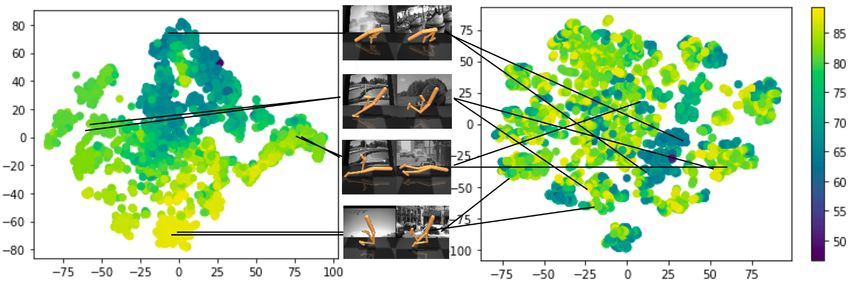
Published as a conference paper at ICLR 2021

Wasserstein metric for the latter, originally used in the context of bisimulation metrics by van Breugel
& Worrell (2001). The pth Wasserstein metric     R is defined between two probability distributions Pi
and Pj as Wp (Pi , Pj ; d) = (inf γ 0 ∈Γ(Pi ,Pj ) S×S d(si , sj )p dγ 0 (si , sj ))1/p , where Γ(Pi , Pj ) is the
set of all couplings of Pi and Pj . This is known as the “earth mover” distance, denoting the cost of
transporting mass from one distribution to another (Villani, 2003). Finally, the bisimulation metric is
the reward difference added to the Wasserstein distance between transition distributions:
Definition 2 (Bisimulation Metric). From Theorem 2.6 in Ferns et al. (2011) with c ∈ [0, 1):
                  d(si , sj ) = max (1 − c) · |Rasi − Rasj | + c · W1 (Psai , Psaj ; d).                     (3)
                                     a∈A

4    Learning Representations for Control with Bisimulation Metrics

                                                         Algorithm 1 Deep Bisimulation for Control (DBC)
                                                         1: for Time t = 0 to ∞ do
                                                         2:    Encode state zt = φ(st )
                                                         3:    Execute action at ∼ π(zt )
                                                         4:    Record data: D ← D ∪ {st , at , st+1 , rt+1 }
                                                         5:    Sample batch Bi ∼ D
                                                         6:    Permute batch: Bj = permute(Bi )
Figure 2: Learning a bisimulation metric represen-       7:    Train policy: EBi [J(π)]          . Algorithm 2
tation: shaded in blue is the main model architecture,
                                                         8:    Train encoder: EBi ,Bj [J(φ)]     . Equation (4)
it is reused for both states, like a Siamese network.
                                                         9:    Train dynamics: J(P̂,φ) = (P̂(φ(st ), at )−z̄t+1 )2
The loss is the reward and discounted transition dis-
tribution distances (using Wasserstein metric W ).
We propose Deep Bisimulation for Control (DBC), a data-efficient approach to learn control policies
from unstructured, high-dimensional states. In contrast to prior work on bisimulation, which typically
aims to learn a distance function of the form d : S × S 7→ R≥0 between states, our aim is instead to
learn representations Z under which `1 distances correspond to bisimulation metrics, and then use
these representations to improve reinforcement learning. Our goal is to learn encoders φ : S 7→ Z
that capture representations of states that are suitable to control, while discarding any information
that is irrelevant for control. Any representation that relies on reconstruction of the state cannot do
this, as these irrelevant details are still important for reconstruction. We hypothesize that bisimulation
metrics can acquire this type of representation, without any reconstruction.
Bisimulation metrics are a useful form of state abstraction, but prior methods to train distance
functions either do not scale to pixel observations (Ferns et al., 2011) (due to the max operator
in Equation (3)), or were only designed for the (fixed) policy evaluation setting (Castro, 2020).
By contrast, we learn improved representations for policy inputs, as the policy improves online.
Our π ∗ -bisimulation metric is learned with gradient decent, and we prove it converges to a fixed
point in Theorem 1 under some assumptions. To train our encoder φ towards our desired relation
d(si , sj ) := ||φ(si ) − φ(sj )||1 , we draw batches of state pairs, and minimise the mean square error
between the on-policy bisimulation metric and `1 distance in the latent space:
                                                                                        2
               J(φ) = ||zi − zj ||1 − |ri − rj | − γW2 P̂(·|z̄i , ai ), P̂(·|z̄j , aj )      ,       (4)
where zi = φ(si ), zj = φ(sj ), r are rewards, and z̄ denotes φ(s) with stop gradients. Equation (4)
also uses a probabilistic dynamics model P̂ which outputs a Gaussian distribution. For this reason,
we use the 2-Wasserstein metric W2 in Equation (4), as opposed to the 1-Wasserstein in Equation (3),
since the W2 metric has a convenient closed form: W2 (N (µi , Σi ), N (µj , Σj ))2 = ||µi − µj ||22 +
   1/2       1/2
||Σi −Σj ||2F , where || · ||F is the Frobenius norm. For all other distances we continue using the
`1 norm. Our model architecture and training is illustrated by Figure 2 and Algorithm 1.
Incorporating control. We combine our rep- Algorithm 2 Train Policy (changes to SAC in blue)
resentation learning approach (Algorithm 1)
with the soft actor-critic (SAC) algorithm 1: Get value: V = mini=1,2 Q̂i (φ̂(s)) − α log π(a|φ(s))
                                                                                                  2
(Haarnoja et al., 2018) to devise a practical 2: Train critics: J(Qi , φ) = (Qi (φ(s)) − r − γV )
                                                3: Train actor: J(π) = α log p(a|φ(s)) − mini=1,2 Qi (φ(s))
reinforcement learning method. We modified 4: Train alpha: J(α) = −α log p(a|φ(s))
SAC slightly in Algorithm 2 to allow the value 5: Update target critics: Q̂i ← τQ Qi + (1 − τQ )Q̂i
function to backprop to our encoder, which 6: Update target encoder: φ̂ ← τφ φ + (1 − τφ )φ̂
can improve performance further (Yarats et al.,
2021; Rakelly et al., 2019). Although, in principle, our method could be combined with any RL

                                                         4
Published as a conference paper at ICLR 2021

algorithm, including the model-free DQN (Mnih et al., 2015), or model-based PETS (Chua et al.,
2018). Implementation details and hyperparameter values of DBC are summarized in the appendix,
Table 2. We train DBC by iteratively updating three components in turn: a policy π (in this case SAC),
an encoder φ, and a dynamics model P̂ (lines 7–9, Algorithm 1). We found a single loss function was
less stable to train. The inputs of each loss function J(·) in Algorithm 1 represents which components
are updated. After each training step, the policy π is used to step in the environment, the data is
collected in a replay buffer D, and a batch is randomly selected to repeat training.

5    Generalization Bounds and Links to Causal Inference
While DBC enables representation learning without pixel reconstruction, it leaves open the question
of how good the resulting representations really are. In this section, we present theoretical analysis
that bounds the suboptimality of a value function trained on the representation learned via DBC.
First, we show that our π ∗ -bisimulation metric converges to a fixed point, starting from the initialized
policy π0 and converging to an optimal policy π ∗ .
Theorem 1. Let met be the space of bounded pseudometrics on S and π a policy that is continuously
improving. Define F : met 7→ met by
                     F(d, π)(si , sj ) = (1 − c)|rsπi − rsπj | + cW (d)(Psπi , Psπj ).        (5)
                               ˜              ∗
Then F has a least fixed point d which is a π -bisimulation metric.
Proof in appendix. As evidenced by Definition 2, the bisimulation metric has no direct dependence on
the state space. Pixels can change, but bisimilarity will stay the same. Instead, bisimilarity is grounded
in a recursion of future transition probabilities and rewards, which is closely related to the optimal
value function. In fact, the bisimulation metric gives tight bounds on the optimal value function
with discount factor γ. We show this using the property that the optimal value function is Lipschitz
with respect to the bisimulation metric, see Theorem 5 in Appendix (Ferns et al., 2004). This result
also implies that the closer two states are in terms of d, ˜ the more likely they are to share the same
optimal actions. This leads us to a generalization bound on the optimal value function of an MDP
constructed from a representation space using bisimulation metrics, ||φ(si ) − φ(sj )||1 := d(s   ˜ i , sj ).
                                                                                             1
We can construct a partition of this space for some  > 0, giving us n partitions where n < (1 − c).
We denote φ as the encoder that maps from the original state space S to each -cluster. This  denotes
the amount of approximation allowed, where large  leads to a more compact bisimulation partition
at the expense of a looser bound on the optimal value function.
Theorem 2 (Value bound based on bisimulation metrics). Given an MDP M̄ constructed by aggre-
gating states in an -neighborhood, and an encoder φ that maps from states in the original MDP M
to these clusters, the optimal value functions for the two MDPs are bounded as
                                                               2
                                |V ∗ (s) − V ∗ (φ(s))| ≤                 .                             (6)
                                                         (1 − γ)(1 − c)
Proof in appendix. As  → 0 the optimal value function of the aggregated MDP converges to the
                                                                                                ˜ i , sj ) ,
original. Further, by defining a learning error for φ, L := supsi ,sj ∈S ||φ(si ) − φ(sj )||1 − d(s
we can update the bound in Theorem 2 to incorporate L: |V ∗ (s) − V ∗ (φ(s))| ≤ (1−γ)(1−c) .
                                                                                         2+2L

MDP dynamics have a strong connection to causal inference and causal graphs, which are directed
acyclic graphs (Jonsson & Barto, 2006; Schölkopf, 2019; Zhang et al., 2020). Specifically, the state
and action at time t causally affect the next state at time t + 1. In this work, we care about the
components of the state space that causally affect current and future reward. Deep bisimulation for
control representations connect to causal feature sets, or the minimal feature set needed to predict a
target variable (Zhang et al., 2020).
Theorem 3 (Connections to causal feature sets (Thm 1 in Zhang et al. (2020))). If we partition
observations using the bisimulation metric, those clusters (a bisimulation partition) correspond to
the causal feature set of the observation space with respect to current and future reward.
This connection tells us that these features are the minimal sufficient statistic of the current and future
reward, and therefore consist of (and only consist of) the causal ancestors of the reward variable r.
Definition 3 (Causal Ancestors). In a causal graph where nodes correspond to variables and directed
edges between a parent node P and child node C are causal relationships, the causal ancestors
AN (C) of a node are all nodes in the path from C to a root node.

                                                     5
Published as a conference paper at ICLR 2021

If there are interventions on distractor variables, or variables that control the rendering function q
and therefore the rendered observation but do not affect the reward, the causal feature set will be
robust to these interventions, and correctly predict current and future reward in the linear function
approximation setting (Zhang et al., 2020). As an example, in autonomous driving, an intervention
can be a change from day to night which affects the observation space but not the dynamics or reward.
Finally, we show that a representation based on the bisimulation metric generalizes to other reward
functions with the same causal ancestors.
Theorem 4 (Task Generalization). Given an encoder φ : S 7→ Z that maps observations to a latent
                                                                 ˜ i , sj ), Z encodes information
bisimulation metric representation where ||φ(si ) − φ(sj )||1 := d(s
about all the causal ancestors of the reward AN (R).
Proof in appendix. This result shows that the learned representation will generalize to unseen reward
functions, as long as the new reward function has a subset of the same causal ancestors. As an
example, a representation learned for a robot to walk will likely generalize to learning to run, because
the reward function depends on forward velocity and all the factors that contribute to forward velocity.
However, that representation will not generalize to picking up objects, as those objects will be ignored
by the learned representation, since they are not likely to be causal ancestors of a reward function
designed for walking. Theorem 4 shows that the learned representation will be robust to spurious
correlations, or changes in factors that are not in AN (R). This complements Theorem 5, that the
representation is a minimal sufficient statistic of the optimal value function, improving generalization
over non-minimal representations.
Theorem 5 (V ∗ is Lipschitz with respect to d).   ˜ Let V ∗ be the optimal value function for a given
discount factor γ. If c ≥ γ, then V is Lipschitz continuous with respect to d˜ with Lipschitz constant
                                    ∗
 1           ˜       ∗
1−c , where d is a π -bisimulation metric.
                                                           1 ˜
                                |V ∗ (si ) − V ∗ (sj )| ≤     d(si , sj ).                         (7)
                                                          1−c
See Theorem 5.1 in Ferns et al. (2004) for proof. We show empirical validation of these findings in
Section 6.2.

6   Experiments
Our central hypothesis is that our non-reconstructive bisimulation based representation learning
approach should be substantially more robust to task-irrelevant distractors. To that end, we evaluate
our method in a clean setting without distractors, as well as a much more difficult setting with
distractors. We compare against several baselines. The first is Stochastic Latent Actor-Critic (SLAC,
Lee et al. (2020)), a state-of-the-art method for pixel observations on DeepMind Control that learns a
dynamics model with a reconstruction loss. The second is DeepMDP (Gelada et al., 2019), a recent
method that also learns a latent representation space using a latent dynamics model, reward model, and
distributional Q learning, but for which they needed a reconstruction loss to scale up to Atari. Finally,
we compare against two methods using the same architecture as ours but exchange our bisimulation
loss with (1) a reconstruction loss (“Reconstruction”) and (2) contrastive predictive coding (Oord
et al., 2018) (“Contrastive”) to ground the dynamics model and learn a latent representation.
6.1 Control with Background Distraction
In this section, we benchmark DBC and the previously described baselines on the DeepMind Control
(DMC) suite (Tassa et al., 2018) in two settings and nine environments (Figure 3), finger_spin,
cheetah_run, and walker_walk and additional environments in the appendix.
Default Setting. Here, the pixel observations have simple backgrounds as shown in Figure 3 (top row)
with training curves for our DBC and baselines. We see SLAC, a recent state-of-the-art model-based
representation learning method that uses reconstruction, generally performs best.
Simple Distractors Setting. Next, we include simple background distractors, shown in Figure 3
(middle row), with easy-to-predict motions. We use a fixed number of colored circles that obey the
dynamics of an ideal gas (no attraction or repulsion between objects) with no collisions. Note the
performance of DBC remains consistent, as other methods start decreasing.
Natural Video Setting. Then, we incorporate natural video from the Kinetics dataset (Kay et al.,
2017) as background (Zhang et al., 2018), shown in Figure 3 (bottom row). The results confirm our
hypothesis: although a number of prior methods can learn effectively in the absence of distractors,

                                                   6
Published as a conference paper at ICLR 2021
finger/spin cheetah/run walker/walk
1000 900
800
800
800 700
600
600 600
AverageReturn
AverageReturn
AverageReturn
500
400 400
400
300
200 200 200
100
0 0 0
0 1 2 3 4 5 6 7 8 0 1 2 3 4 5 6 7 8 0 1 2 3 4 5 6 7 8
Environment Steps 1e5 Environment Steps 1e5 Environment Steps 1e5
finger/spin cheetah/run walker/walk
600
800
800
500 700
600
600 400
AverageReturn
AverageReturn
AverageReturn
500
300
400 400
200 300
200 200
100
100
0 0 0
0 1 2 3 4 5 6 7 8 0 1 2 3 4 5 6 7 8 0 1 2 3 4 5 6 7 8
Environment Steps 1e5 Environment Steps 1e5 Environment Steps 1e5
finger/spin cheetah/run walker/walk
700
300
800 600
250
500
600
200
AverageReturn
AverageReturn
AverageReturn
400
400 150
300
100
200
200
50
100
0 0 0
0 1 2 3 4 5 6 7 8 0 1 2 3 4 5 6 7 8 0 1 2 3 4 5 6 7 8
Environment Steps 1e5 Environment Steps 1e5 Environment Steps 1e5
Figure 3: Left observations: Pixel observations in DMC in the default setting (top row) of the finger spin (left
column), cheetah (middle column), and walker (right column), with simple distractors (middle row), and natural
video distractors (bottom row). Right training curves: Results comparing out DBC method to baselines on 10
seeds with 1 standard error shaded in the default setting. The grid-location of each graph corresponds to the
grid-location of each observation.
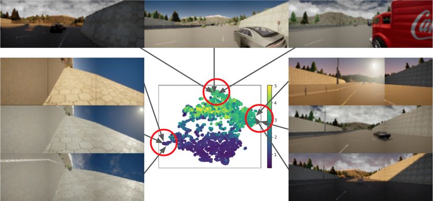
Figure 4: t-SNE of latent spaces learned with a bisimulation metric (left t-SNE) and VAE (right t-SNE)
after training has completed, color-coded with predicted state values (higher value yellow, lower value purple).
Neighboring points in the embedding space learned with a bisimulation metric have similar states and correspond
to observations with the same task-related information (depicted as pairs of images with their corresponding
embeddings), whereas no such structure is seen in the embedding space learned by VAE, where the same image
pairs are mapped far away from each other.
when complex distractions are introduced, our non-reconstructive bisimulation based method attains
substantially better results.
To visualize the representation learned with our bisimulation metric loss function in Equation (4), we
use a t-SNE plot (Figure 4). We see that even when the background looks drastically different, our en-
coder learns to ignore irrelevant information and maps observations with similar robot configurations
near each other. See Appendix D for another visualization.
6.2 Generalization Experiments
We test generalization of our learned representation in two ways. First, we show that the learned
representation space can generalize to different types of distractors, by training with simple distractors
and testing on the natural video setting. Second, we show that our learned representation can be
useful reward functions other than those it was trained for.
Generalizing over backgrounds. We first train on the simple distractors setting and eval-
uate on natural video. Figure 5 shows an example of the simple distractors setting
and performance during training time of two experiments, blue being the zero-shot transfer to the
7
Published as a conference paper at ICLR 2021
natural video setting, and orange the baseline which trains on natural video. This result
empirically validates that the representations learned by DBC are able to effectively learn to ignore
the background, regardless of what the background contains or how dynamic it is.
Generalizing over reward functions. We evaluate (Figure 5) the generalization capabilities of
the learned representation by training SAC with new reward functions walker_stand and
walker_run using the fixed representation learned from walker_walk. This is empirical
evidence that confirms Theorem 4: if the new reward functions are causally dependent on a subset of
the same factors that determine the original reward function, then our representation is sufficient.
walker_walk walker_stand walker_run
300
700
1000
SAC trained on observation
900 SAC trained with frozen bisim encoder
600
250 SAC trained with frozen DeepMDP encoder
800
500 700 200
episode_reward
episode_reward
episode_reward
400 600
150
500
300
400
100
200
Bisim: Transfer ideal gas to kinetics 300
SAC trained on observation
100
Bisim: Trained on kinetics 200 SAC trained with frozen bisim encoder 50
DeepMDP: Transfer ideal gas to kinetics SAC trained with frozen DeepMDP encoder
0 100
0 200000 400000 600000 800000 1000000 0 200000 400000 600000 800000 1000000 0 200000 400000 600000 800000 1000000
step step step
Figure 5: Generalization of a model trained on simple distractors environment and evaluated on
kinetics (left). Generalization of an encoder trained on walker_walk environment and evaluated on
walker_stand (center) and walker_run (right), all in the simple distractors setting. 10 seeds, 1
standard error shaded.
6.3 Comparison with other Bisimulation Encoders
Even though the purpose of bisimulation metrics by Castro (2020) is learning distances d, not
representation spaces Z, it nevertheless implements d with function approximation: d(si , sj ) =
ψ φ(si ), φ(sj ) by
encoding observations with φ before
computing distances with ψ, trained as:
2
J(φ, ψ) = ψ φ(si ), φ(sj ) − |ri − rj | − γ ψ̂ φ̂ P(si , π(si )) , φ̂ P(sj , π(sj )) , (8)
where φ̂ and ψ̂ are target networks. A natural question is: how walker_walk with natural video
700 DBC
does the encoder φ above perform in control tasks? We com- Castro
600
bine φ above with our policy in Algorithm 2 and use the same
500
network ψ (single hidden layer 729 wide). Figure 6 shows rep-
episode_reward
resentations from Castro (2020) can learn control (surprisingly 400
well given it was not designed to), but our method learns faster. 300
Further, our method is simpler: by comparing Equation (8) 200
to Equation (4), our method uses the `1 distance between the 100
encoding instead of introducing an addition network ψ. 0
0 100000 200000 300000 400000
step
500000 600000 700000 800000
6.4 Autonomous Driving with Visual Redundancy Figure 6: Bisim. results. Blue is DBC
and orange is Castro (2020).
Real-world control systems such as robotics
and autonomous vehicles must contend with
a huge variety of task-irrelevant information,
such as irrelevant objects (e.g. clouds) and ir-
relevant details (e.g. obstacle color). To eval-
uate DBC on tasks with more realistic obser- Figure 7: The driving task is to drive the red ego car
vations, we construct a highway driving sce- (left) safely in traffic (middle) along a highway (right).
nario with photo-realistic visual observations using the CARLA simulator (Dosovitskiy et al.,
2017) shown in Figure 7. The agent’s goal is to drive as far as possible along CARLA’s
Town04’s figure-8 the highway in 1000 time-steps without colliding into the 20 other moving
vehicles or barriers. Our objective function rewards highway progression and penalises collisions:
>
rt = vego ûhighway · ∆t − λi · impulse − λs · |steer|, where vego is the velocity vector of the ego vehi-
cle, projected onto the highway’s unit vector ûhighway , and multiplied by time discretization ∆t = 0.05
to measure highway progression in meters. Collisions result in impulses ∈ R+ , measured in Newton-
seconds. We found a steering penalty steer ∈ [−1, 1] helped, and used weights λi = 10−4 and
λs = 1. While more specialized objectives exist like lane-keeping, this experiment’s purpose is only
to compare representations with observations more characteristic of real robotic tasks. We use five
cameras on the vehicle’s roof, each with 60 degree views. By concatenating the images together, our
vehicle has a 300 degree view, observed as 84 × 420 pixels. Code and install instructions in appendix.
8
Published as a conference paper at ICLR 2021

  Results in Figure 9 compare the same baselines as before, except for SLAC which is easily distracted
  (Figure 3). Instead we used SAC, which does not explicitly learn a representation, but performs
  surprisingly well from raw images. DeepMDP performs well too, perhaps given its similarly to
  bisimulation. But, Reconstruction and Contrastive methods again perform poorly with complex
  images. More intuitive metrics are in Table 1 and Figure 8 depicts the representation space as a t-SNE
  with corresponding observations. Each run took 12 hours on a GTX 1080 GPU.

   Figure 8: A t-SNE diagram of encoded first-person driving observations after 10k training steps of Algorithm 1,
   color coded by value (V in Algorithm 2). Top: the learned representation identifies an obstacle on the right
   side. Whether that obstacle is a dark wall, bright car, or truck is task-irrelevant: these states are behaviourally
   equivalent. Left: the ego vehicle has flipped onto its left side. The different wall colors, due to a setting sun, is
   irrelevant: all states are equally stuck and low-value (purple t-SNE color). Right: clear highway driving. Clouds
   and sun position are irrelevant.
                                            carla                  Figure 9: Performance comparison with 3 seeds on the
                           Contrastive                             driving task. Our DBC method (red) performs better
                 175       Reconstruction                          than DeepMDP (purple) or learning direct from pixels
                 150       SAC                                     without a representation (SAC, green), and much better
                 125       DeepMDP                                 than contrastive methods (blue). Our method’s final
episode_reward

                           DBC (ours)                              performance is 46.8% better than the next best baseline.
                 100
                  75                                               Table 1: Driving metrics, averaged over 100 episodes,
                                                                   after 100k training steps, with standard error. Arrow
                  50
                                                                   direction indicates if metric desired larger or smaller.
                  25                                                                              SAC            DeepMDP        DBC (ours)
                   0                                                   successes (100m) ↑
                                                                       distance (m)     ↑
                                                                                                  12%
                                                                                              123.2 ± 7.43
                                                                                                                   17%
                                                                                                               106.7 ± 11.1
                                                                                                                                   24%
                                                                                                                               179.0 ± 11.4
                                                                       crash intensity ↓      4604 ± 30.7      1958 ± 15.6      2673 ± 38.5
                       0    20000     40000 60000   80000 100000       average steer    ↓   16.6% ± 0.019%   10.4% ± 0.015%   7.3% ± 0.012%
                                           step                        average brake    ↓   1.3% ± 0.006%     4.3% ± 0.033%   1.6% ± 0.022%

   7               Discussion
  This paper presents Deep Bisimulation for Control: a new representation learning method that
  considers downstream control. Observations are encoded into representations that are invariant to
  different task-irrelevant details in the observation. We show this is important when learning control
  from outdoor images, or otherwise images with background “distractions”. In contrast to other
  bisimulation methods, we show performance gains when distances in representation space match the
  bisimulation distance between observations.
   Future work: Several options exist for future work. First, our latent dynamics model P̂ was only
   used for training our encoder in Equation (4), but could also be used for multi-step planning in latent
   space. Second, estimating uncertainty could also be important to produce agents that can work in
   the real world, perhaps via an ensemble of models {P̂k }Kk=1 , to detect—and adapt to—distributional
   shifts between training and test observations. Third, an undressed issue is that of partially observed
   settings (that assumed approximately full observability by using stacked images), possibly using
   explicit memory or implicit memory such as an LSTM. Finally, investigating which metrics (L1 or
   L2) and dynamics distributions (Gaussians or not) would be beneficial.

                                                                   9
Published as a conference paper at ICLR 2021

References
Pablo Samuel Castro. Scalable methods for computing state similarity in deterministic Markov
  decision processes. In Association for the Advancement of Artificial Intelligence (AAAI), 2020.
Ting Chen, Simon Kornblith, Mohammad Norouzi, and Geoffrey Hinton. A simple framework for
  contrastive learning of visual representations. In International Conference on Machine Learning
  (ICML), pp. 1597–1607. PMLR, 2020.
Kurtland Chua, Roberto Calandra, Rowan McAllister, and Sergey Levine. Deep reinforcement
  learning in a handful of trials using probabilistic dynamics models. In Neural Information
  Processing Systems (NeurIPS), pp. 4754–4765, 2018.
Alexey Dosovitskiy, German Ros, Felipe Codevilla, Antonio Lopez, and Vladlen Koltun. CARLA:
  An open urban driving simulator. In Conference on Robot Learning (CoRL), pp. 1–16, 2017.
Simon S. Du, Akshay Krishnamurthy, Nan Jiang, Alekh Agarwal, Miroslav Dudík, and John Langford.
  Provably efficient RL with rich observations via latent state decoding. Computing Research
  Repository (CoRR), abs/1901.09018, 2019. URL http://arxiv.org/abs/1901.09018.
Norm Ferns, Prakash Panangaden, and Doina Precup. Metrics for finite Markov decision processes.
  In Uncertainty in Artificial Intelligence (UAI), pp. 162–169, 2004. ISBN 0-9749039-0-6. URL
  http://dl.acm.org/citation.cfm?id=1036843.1036863.
Norm Ferns, Prakash Panangaden, and Doina Precup. Bisimulation metrics for continuous Markov
  decision processes. Society for Industrial and Applied Mathematics, 40(6):1662–1714, December
  2011. ISSN 0097-5397. doi: 10.1137/10080484X. URL https://doi.org/10.1137/
  10080484X.
Norman Ferns and Doina Precup. Bisimulation metrics are optimal value functions. In Uncertainty
  in Artificial Intelligence (UAI), pp. 210–219, 2014.
Carles Gelada, Saurabh Kumar, Jacob Buckman, Ofir Nachum, and Marc G. Bellemare. DeepMDP:
  Learning continuous latent space models for representation learning. In Kamalika Chaudhuri and
  Ruslan Salakhutdinov (eds.), International Conference on Machine Learning (ICML), volume 97,
  pp. 2170–2179, Jun 2019.
Robert Givan, Thomas L. Dean, and Matthew Greig. Equivalence notions and model minimization in
  Markov decision processes. Artificial Intelligence, 147:163–223, 2003.
Tuomas Haarnoja, Aurick Zhou, Pieter Abbeel, and Sergey Levine. Soft actor-critic: Off-policy
  maximum entropy deep reinforcement learning with a stochastic actor. In International Conference
  on Machine Learning (ICML), pp. 1861–1870. PMLR, 2018.
Danijar Hafner, Timothy Lillicrap, Ian Fischer, Ruben Villegas, David Ha, Honglak Lee, and James
  Davidson. Learning latent dynamics for planning from pixels. In International Conference on
  Machine Learning (ICML), pp. 2555–2565. PMLR, 2019.
Olivier J Hénaff, Aravind Srinivas, Jeffrey De Fauw, Ali Razavi, Carl Doersch, SM Eslami, and
  Aaron van den Oord. Data-efficient image recognition with contrastive predictive coding. In
  International Conference on Machine Learning (ICML), pp. 4182–4192. PMLR, 2020.
Rico Jonschkowski and Oliver Brock. Learning state representations with robotic priors. Autonomous
  Robots, 39(3):407–428, 2015.
Anders Jonsson and Andrew Barto. Causal graph based decomposition of factored MDPs. J. Mach.
  Learn. Res., 7:2259–2301, December 2006. ISSN 1532-4435.
Will Kay, João Carreira, Karen Simonyan, Brian Zhang, Chloe Hillier, Sudheendra Vijayanarasimhan,
  Fabio Viola, Tim Green, Trevor Back, Paul Natsev, Mustafa Suleyman, and Andrew Zisserman.
  The kinetics human action video dataset. Computing Research Repository (CoRR), 2017. URL
  http://arxiv.org/abs/1705.06950.
Sascha Lange and Martin Riedmiller. Deep auto-encoder neural networks in reinforcement learning.
  In International Joint Conference on Neural Networks (IJCNN), pp. 1–8. IEEE, 2010.
Sascha Lange, Martin Riedmiller, and Arne Voigtländer. Autonomous reinforcement learning on raw
  visual input data in a real world application. In International Joint Conference on Neural Networks
  (IJCNN), pp. 1–8, 2012. doi: 10.1109/IJCNN.2012.6252823.
K. G. Larsen and A. Skou. Bisimulation through probabilistic testing (preliminary report). In
  Symposium on Principles of Programming Languages, pp. 344–352. Association for Computing
  Machinery, 1989. ISBN 0897912942. doi: 10.1145/75277.75307. URL https://doi.org/
  10.1145/75277.75307.

                                                10
Published as a conference paper at ICLR 2021
Michael Laskin, Aravind Srinivas, and Pieter Abbeel. CURL: Contrastive unsupervised representa-
tions for reinforcement learning. In International Conference on Machine Learning (ICML), pp.
5639–5650. PMLR, 2020.
Alex Lee, Anusha Nagabandi, Pieter Abbeel, and Sergey Levine. Stochastic latent actor-critic: Deep
reinforcement learning with a latent variable model. In Neural Information Processing Systems
(NeurIPS), volume 33, pp. 741–752, 2020. URL https://proceedings.neurips.cc/
paper/2020/file/08058bf500242562c0d031ff830ad094-Paper.pdf.
Lihong Li, Thomas J Walsh, and Michael L Littman. Towards a unified theory of state abstraction for
MDPs. In International Symposium on Artificial Intelligence and Mathematics (ISAIM), 2006.
Volodymyr Mnih, Koray Kavukcuoglu, David Silver, Andrei A. Rusu, Joel Veness, Marc G.
Bellemare, Alex Graves, Martin Riedmiller, Andreas K. Fidjeland, Georg Ostrovski, Stig Pe-
tersen, Charles Beattie, Amir Sadik, Ioannis Antonoglou, Helen King, Dharshan Kumaran,
Daan Wierstra, Shane Legg, and Demis Hassabis. Human-level control through deep rein-
forcement learning. Nature, 518(7540):529–533, February 2015. ISSN 00280836. URL
http://dx.doi.org/10.1038/nature14236.
Aaron van den Oord, Yazhe Li, and Oriol Vinyals. Representation learning with contrastive predictive
coding. arXiv preprint arXiv:1807.03748, 2018.
Kate Rakelly, Aurick Zhou, Deirdre Quillen, Chelsea Finn, and Sergey Levine. Efficient off-policy
meta-reinforcement learning via probabilistic context variables. In International conference on
Machine Learning (ICML), pp. 5331–5340. PMLR, 2019.
Bernhard Schölkopf. Causality for machine learning, 2019.
Yuval Tassa, Yotam Doron, Alistair Muldal, Tom Erez, Yazhe Li, Diego de Las Casas, David
Budden, Abbas Abdolmaleki, Josh Merel, Andrew Lefrancq, Timothy Lillicrap, and Martin
Riedmiller. DeepMind control suite. Technical report, DeepMind, January 2018. URL https:
//arxiv.org/abs/1801.00690.
Jonathan Taylor, Doina Precup, and Prakash Panagaden. Bounding performance loss in approximate
MDP homomorphisms. In Neural Information Processing (NeurIPS), pp. 1649–1656, 2009.
Franck van Breugel and James Worrell. Towards quantitative verification of probabilistic transition
systems. In Fernando Orejas, Paul G. Spirakis, and Jan van Leeuwen (eds.), Automata, Languages
and Programming, pp. 421–432. Springer, 2001. ISBN 978-3-540-48224-6. doi: 10.1007/
3-540-48224-5_35.
Aäron van den Oord, Yazhe Li, and Oriol Vinyals. Representation learning with contrastive predictive
coding. ArXiv, abs/1807.03748, 2018.
Cédric Villani. Topics in optimal transportation. American Mathematical Society, 01 2003.
Niklas Wahlström, Thomas Schön, and Marc Deisenroth. From pixels to torques: Policy learning
with deep dynamical models. arXiv preprint arXiv:1502.02251, 2015.
Manuel Watter, Jost Springenberg, Joschka Boedecker, and Martin Riedmiller. Embed to control:
A locally linear latent dynamics model for control from raw images. In Neural Information
Processing Systems (NeurIPS), pp. 2728–2736, 2015.
Denis Yarats and Ilya Kostrikov. Soft actor-critic (SAC) implementation in PyTorch. https:
//github.com/denisyarats/pytorch_sac, 2020.
Denis Yarats, Amy Zhang, Ilya Kostrikov, Brandon Amos, Joelle Pineau, and Rob Fergus. Improving
sample efficiency in model-free reinforcement learning from images. In Association for the
Advancement of Artificial Intelligence (AAAI), 2021.
Amy Zhang, Yuxin Wu, and Joelle Pineau. Natural environment benchmarks for reinforcement
learning. Computing Research Repository (CoRR), abs/1811.06032, 2018. URL http://arxiv.
org/abs/1811.06032.
Amy Zhang, Clare Lyle, Shagun Sodhani, Angelos Filos, Marta Kwiatkowska, Joelle Pineau, Yarin
Gal, and Doina Precup. Invariant causal prediction for block MDPs. In International Conference
on Machine Learning (ICML), 2020.
11Published as a conference paper at ICLR 2021
A Additional Theorems and Proofs
Theorem 1. Let met be the space of bounded pseudometrics on S and π ∈ Π a policy that is
continuously improving in the space of policies Π. Define F : met × Π 7→ met by
F(d, π)(si , sj ) = (1 − c)|rsπi − rsπj | + cW (d)(Psπi , Psπj ). (9)
Then F has a least fixed point d˜ which is a π ∗ -bisimulation metric.
Proof. Ideally, to prove this theorem we show that F is monotonically increasing and continuous, and
apply Fixed Point Theorem to show the existence of a fixed point that F converges to. Unfortunately,
we can show that F under π as π monotonically converges to π ∗ is not also monotonic, unlike the
original bisimulation metric setting (Ferns et al., 2004) and the policy evaluation setting (Castro,
2020). We start the iterates F n from bottom ⊥, denoted as F n (⊥). In Ferns et al. (2004) the maxa∈A
can be thought of as learning a policy between every two pairs of states to maximize their distance,
and therefore this distance can only stay the same or grow over iterations of F. In Castro (2020), π is
fixed, and under a deterministic MDP it can also be shown that distance between states dn (si , sj )
will only expand, not contract as n increases. In the policy iteration setting, however, with π starting
from initialization π0 and getting updated: X
a πk−1 0
πk (s) = arg max [rss0 + γV (s )], (10)
a∈A
s0 ∈S
π
k−1
there is no guarantee that the distance between two states dn−1 (si , sj ) < dπnk (si , sj ) under policy
iterations πk−1 , πk and distance metric iterations dn−1 , dn for k, n ∈ N, which is required for
monotonicity.
Instead, we show that using the policy improvement theorem which gives us
V πk (s) ≥ V πk−1 (s), ∀s ∈ S, (11)
π will converge to a fixed point using the Fixed Point Theorem, and taking the result by Castro (2020)
that F π has a fixed point for every π ∈ Π, we can show that a fixed point bisimulation metric will be
found with policy iteration.
Theorem 2. Given a new aggregated MDP M̄ constructed by aggregating states in an -
neighborhood, and an encoder φ that maps from states in the original MDP M to these clusters, the
optimal value functions for the two MDPs are bounded as
2
|V ∗ (s) − V ∗ (φ(s))| ≤ . (12)
(1 − γ)(1 − c)
Proof. From Theorem 5.1 in Ferns et al. (2004) we have:
˜ + γ ˜
(1 − c)|V ∗ (s) − V ∗ (φ(s))| ≤ g(s, d) max g(u, d)
1 − γ u∈S
where g is the average distance between a state and all other states in its equivalence class under the
˜ By specifying a -neighborhood for each cluster of states we can replace g:
bisimulation metric d.
γ
(1 − c)|V ∗ (s) − V ∗ (φ(s))| ≤ 2 + 2
1−γ
1 γ
|V ∗ (s) − V ∗ (φ(s))| ≤ (2 + 2)
1−c 1−γ
2
= .
(1 − γ)(1 − c)
Theorem 4. Given an encoder φ : S 7→ Z that maps observations to a latent bisimulation metric
˜ i , sj ), Z encodes information about all the causal
representation where ||φ(si ) − φ(sj )||1 := d(s
ancestors of the reward AN (R).
Proof. We assume a MDP with a state space S := {S 1 , ..., S K } that can be factorized into K
variables with 1-step causal transition dynamics described by a causal graph G (example in Figure 10).
We break the proof up into two parts: 1) show that if a factor S i ∈ / AN (R) changes, the bisimulation
distance between the original state s and the new state s0 is 0. and 2) show that if a factor S j ∈ AN (R)
changes, the bisimulation distance can be > 0.
12Published as a conference paper at ICLR 2021
Figure 10: Causal graph of transition dynamics. Reward depends only on s1 as a causal parent, but s1
causally depends on s2 , so AN(R) is the set {s1 , s2 }.
1) If S i ∈
/ AN (R), an intervention on that factor does not affect current or future reward.
˜ i , sj ) = max(1 − c)|ra − ra | + cW (d)(P
d(s ˜ a , Pa )
si sj si sj
a∈A
˜ a , P a ) si and sj have the same reward.
= max cW (d)(Psi sj
a∈A
If S i does not affect future reward, then states si and sj will have the same future reward conditioned
on all future actions. This gives us
˜ s0 ) = 0.
d(s,
j
2) If there is an intervention on S ∈ AN (R) then current and/or future reward can change. If
current reward changes, then we already have maxa∈A (1 − c)|rsai − rsaj | > 0, giving us d(s ˜ i , sj ) >
0. If only future reward changes, then those future states will have nonzero bisimilarity, and
maxa∈A W (d)(P ˜ a , P a ) > 0, giving us d(s˜ i , sj ) > 0.
si sj
B Definition of State
Since we are concerned primarily with learning from image observations, we could explicitly
distinguish the image observation space O from an unknown state space S. However, since we are
not tackling the general POMDP problem, we consider the Block MDP (Du et al., 2019), which
assumes the state space is latent, and that we are instead given access to an observation space O
and rendering function q : S 7→ O. The crucial assumption that distinguishes the Block MDP from
partially observable MDPs is the following:
Assumption 1 (Block structure (Du et al., 2019)). Each observation o uniquely determines its
generating state s. That is, the observation space O can be partitioned into disjoint blocks Os , each
containing the support of the conditional distribution q(o|s).
This assumption gives us the Markov property in the observation space o ∈ O. As an example,
one can think of the proprioceptive state consisting of positions and velocities of actuators as the
underlying state, and stacked pixel observations from a specific camera angle as a particular rendering
function and corresponding observation space.
C Additional DMC Results
In Figure 11 we show performance on the default setting on 9 different environments from DMC.
Figures 12 and 13 give performance on the simple distractors and natural video settings for all 9
environments.
13Published as a conference paper at ICLR 2021
cartpole/swingup cheetah/run 1000
finger/spin
900
800
800
800
700 700
600 600
Contrastive 600 Contrastive
Contrastive
AverageReturn
AverageReturn
500 Reconstruction 500 Reconstruction Reconstruction
AverageReturn
Bisim Bisim Bisim
400 DeepMDP 400 DeepMDP 400 DeepMDP
SLAC SLAC SLAC
300 300
200
200 200
100
100
0 0
0
0 1 2 3 4 5 6 7 8 0 1 2 3 4 5 6 7 8 0 1 2 3 4 5 6 7 8
Environment Steps 1e5 Environment Steps 1e5 Environment Steps 1e5
hopper/hop hopper/stand reacher_easy
350 Contrastive
Contrastive Contrastive
Reconstruction 800 Reconstruction Reconstruction
250 Bisim Bisim 300 Bisim
DeepMDP 700 DeepMDP DeepMDP
SLAC SLAC SLAC
200 600 250
episode_reward
AverageReturn
AverageReturn
500
150 200
400
150
100 300
200 100
50
100
50
0 0
0 1 2 3 4 5 6 7 8 0 1 2 3 4 5 6 7 8 0 100000 200000 300000 400000 500000 600000 700000 800000
Environment Steps 1e5 Environment Steps 1e5 step
walker/run 1000
walker/stand walker/walk
600 Contrastive Contrastive
Reconstruction 900 Reconstruction
Bisim 800 Bisim
500 DeepMDP 800 DeepMDP
SLAC SLAC
700
400
Contrastive 600
AverageReturn
AverageReturn
600 Reconstruction
AverageReturn
Bisim
300 500 DeepMDP 400
SLAC
400
200
300 200
100
200
100 0
0
0 1 2 3 4 5 6 7 8 0 1 2 3 4 5 6 7 8 0 1 2 3 4 5 6 7 8
Environment Steps 1e5 Environment Steps 1e5 Environment Steps 1e5
Figure 11: Results for DBC in the default setting, in comparison to baselines with reconstruction loss,
contrastive loss, and SLAC on 10 seeds with 1 standard error shaded.
cartpole/swingup cheetah/run finger/spin
Contrastive 600
800 Reconstruction
Bisim 800
700 DeepMDP 500
SLAC
600
400 600
AverageReturn
AverageReturn
500
AverageReturn
300
400 400
300 200
200 200
100
100
0 0
0
0 1 2 3 4 5 6 7 8 0 1 2 3 4 5 6 7 8 0 1 2 3 4 5 6 7 8
Environment Steps 1e5 Environment Steps 1e5 Environment Steps 1e5
hopper/hop hopper/stand reacher/easy
Contrastive Contrastive 600 Contrastive
60 Reconstruction Reconstruction Reconstruction
Bisim 500 Bisim Bisim
50 DeepMDP DeepMDP 500 DeepMDP
SLAC SLAC SLAC
400
40 400
AverageReturn
AverageReturn
AverageReturn
300
30
300
20 200
200
10 100
0 100
0
0 1 2 3 4 5 6 7 8 0 1 2 3 4 5 6 7 8 0 1 2 3 4 5 6 7 8
Environment Steps 1e5 Environment Steps 1e5 Environment Steps 1e5
walker/run 1000 walker/stand walker/walk
350
Contrastive Contrastive
Reconstruction 900 Reconstruction 800
300 Bisim Bisim
DeepMDP 800 DeepMDP 700
SLAC SLAC
250 600
700
AverageReturn
AverageReturn
AverageReturn
200 600 500
500 400
150
400 300
100
300 200
50 200 100
100 0
0 1 2 3 4 5 6 7 8 0 1 2 3 4 5 6 7 8 0 1 2 3 4 5 6 7 8
Environment Steps 1e5 Environment Steps 1e5 Environment Steps 1e5
Figure 12: Results for DBC in the simple distractors setting, in comparison to baselines with
reconstruction loss, contrastive loss, DeepMDP, and SLAC on 10 seeds with 1 standard error shaded.
14You can also read