Model Fusion via Optimal Transport - arXiv.org
←
→
Page content transcription
If your browser does not render page correctly, please read the page content below

Model Fusion via Optimal Transport

                                                            Sidak Pal Singh                               Martin Jaggi
                                                                 EPFL                                        EPFL
                                                        contact@sidakpal.com                         martin.jaggi@epfl.ch
arXiv:1910.05653v4 [cs.LG] 19 Jun 2020

                                                                                       Abstract

                                                  Combining different models is a widely used paradigm in machine learning appli-
                                                  cations. While the most common approach is to form an ensemble of models and
                                                  average their individual predictions, this approach is often rendered infeasible by
                                                  given resource constraints in terms of memory and computation, which grow lin-
                                                  early with the number of models. We present a layer-wise model fusion algorithm
                                                  for neural networks that utilizes optimal transport to (soft-) align neurons across
                                                  the models before averaging their associated parameters.
                                                      We show that this can successfully yield “one-shot” knowledge transfer (i.e,
                                                  without requiring any retraining) between neural networks trained on heteroge-
                                                  neous non-i.i.d. data. In both i.i.d. and non-i.i.d. settings , we illustrate that our
                                                  approach significantly outperforms vanilla averaging, as well as how it can serve as
                                                  an efficient replacement for the ensemble with moderate fine-tuning, for standard
                                                  convolutional networks (like VGG11), residual networks (like R ES N ET 18), and
                                                  multi-layer perceptrons on CIFAR10 and MNIST. Finally, our approach also pro-
                                                  vides a principled way to combine the parameters of neural networks with different
                                                  widths, and we explore its application for model compression.

                                         1   Introduction
                                         If two neural networks had a child, what would be its weights? In this work, we study the fusion of
                                         two parent neural networks—which were trained differently but have the same number of layers—into
                                         a single child network. We further focus on performing this operation in a one-shot manner, based on
                                         the network weights only, so as to minimize the need of any retraining.
                                         This fundamental operation of merging several neural networks into one contrasts other widely used
                                         techniques for combining machine learning models:
                                         Ensemble methods have a very long history . They combine the outputs of several different models as
                                         a way to improve the prediction performance and robustness. However, this requires maintaining
                                         the K trained models and running each of them at test time (say, in order to average their outputs).
                                         This approach thus quickly becomes infeasible for many applications with limited computational
                                         resources, especially in view of the ever-growing size of modern deep learning models.
                                         The simplest way to fuse several parent networks into a single network of the same size is direct weight
                                         averaging, which we refer to as vanilla averaging; here for simplicity, we assume that all network
                                         architectures are identical. Unfortunately, neural networks are typically highly redundant in their
                                         parameterizations, so that there is no one-to-one correspondence between the weights of two different
                                         neural networks, even if they would describe the same function of the input. In practice, vanilla
                                         averaging is known to perform very poorly on trained networks whose weights differ non-trivially.
                                         Finally, a third way to combine two models is distillation, where one network is retrained on its
                                         training data, while jointly using the output predictions of the other ‘teacher’ network on those
                                         samples. Such a scenario is considered infeasible in our setting, as we aim for approaches not

                                         Accepted at NeurIPS 2019: Optimal Transport & Machine Learning workshop.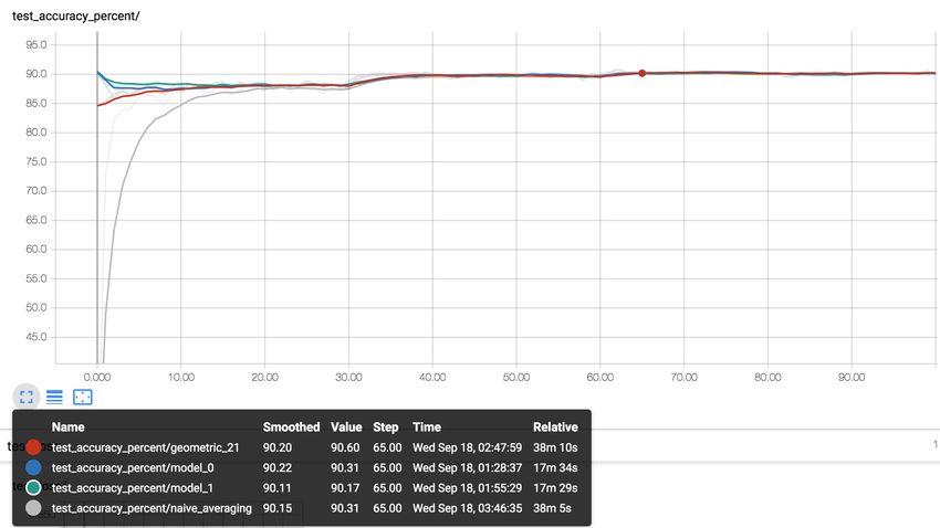
requiring the sharing of training data. This requirement is particularly crucial if the training data is to
be kept private, like in federated learning applications, or is unavailable due to e.g. legal reasons.
Contributions. We propose a novel layer-wise approach of aligning the neurons and weights of
several differently trained models, for fusing them into a single model of the same architecture.
Our method relies on optimal transport (OT) [1, 2], to minimize the transportation cost of neurons
present in the layers of individual models, measured by the similarity of activations or incoming
weights. The resulting layer-wise averaging scheme can be interpreted as computing the Wasserstein
barycenter [3, 4] of the probability measures defined at the corresponding layers of the parent models.
We empirically demonstrate that our method succeeds in the one-shot merging of networks of different
weights, and in all scenarios significantly outperforms vanilla averaging. More surprisingly, we
also show that our method succeeds in merging two networks that were trained for slightly different
tasks (such as using a different set of labels). The method is able to “inherit” abilities unique to one
of the parent networks, while outperforming the same parent network on the task associated with
the other network. Further, we illustrate how it can serve as a data-free and algorithm independent
post-processing tool for structured pruning. Finally, we show that OT fusion, with mild fine-tuning,
can act as efficient proxy for the ensemble, whereas vanilla averaging fails for more than two models.
Extensions and Applications. The method serves as a new building block for enabling several
use-cases: (1) The adaptation of a global model to personal training data. (2) Fusing the parameters
of a bigger model into a model of smaller size and vice versa. (3) Federated or decentralized learning
applications, where training data is not allowed to be shared due to privacy reasons or simply due
to its large size. In general, improved model fusion techniques such as ours have strong potential
towards encouraging model exchange as opposed to data exchange, to improve privacy & reduce
communication costs.

2   Related Work

Ensembling. Ensemble methods [5–7] have long been in use in deep learning and machine learning
in general. However, given our goal is to obtain a single model, it is assumed infeasible to maintain
and run several trained models as needed here.
Distillation. Another line of work by Hinton et al. [8], Buciluǎ et al. [9], Schmidhuber [10] proposes
distillation techniques. Here the key idea is to employ the knowledge of a pre-trained teacher network
(typically larger and expensive to train) and transfer its abilities to a smaller model called the student
network. During this transfer process, the goal is to use the relative probabilities of misclassification
of the teacher as a more informative training signal.
While distillation also results in a single model, the main drawback is its computational complexity—
the distillation process is essentially as expensive as training the student network from scratch, and
also involves its own set of hyper-parameter tuning. In addition, distillation still requires sharing the
training data with the teacher (as the teacher network can be too large to share), which we avoid here.
In a different line of work, Shen et al. [11] propose an approach where the student network is forced
to produce outputs mimicking the teacher networks, by utilizing Generative Adversarial Network [12].
This still does not resolve the problem of high computational costs involved in this kind of knowledge
transfer. Further, it does not provide a principled way to aggregate the parameters of different models.
Relation to other network fusion methods. Several studies have investigated a method to merge
two trained networks into a single network without the need for retraining [13–15]. Leontev et al.
[15] propose Elastic Weight Consolidation, which formulates an assignment problem on top of
diagonal approximations to the Hessian matrices of each of the two parent neural networks. Their
method however only works when the weights of the parent models are already close, i.e. share a
significant part of the training history [13, 14], by relying on SGD with periodic averaging, also called
local SGD [16]. Nevertheless, their empirical results [15] do not improve over vanilla averaging.
Alignment-based methods. Recently, Yurochkin et al. [17] independently proposed a Bayesian non-
parametric framework that considers matching the neurons of different MLPs in federated learning.
In a concurrent work, Wang et al. [18] extend [17] to more realistic networks including CNNs, also
with a specific focus on federated learning. In contrast, we develop our method from the lens of
optimal transport (OT), which lends us a simpler approach by utilizing Wasserstein barycenters. The

                                                    2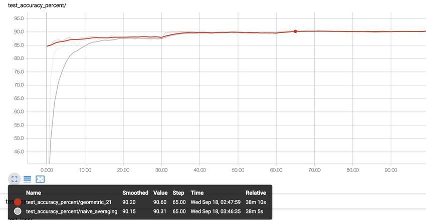
method of aligning neurons employed in both lines of work form instances for the choice of ground
metric in OT. Overall, we consider model fusion in general, beyond federated learning. For instance,
we show applications of fusing different sized models (e.g., for structured pruning) as well as the
compatibility of our method to serve as an initialization for distillation. From a practical point, our
approach is number of layer times more efficient and also applies to ResNets.
To conclude, the application of Wasserstein barycenters for averaging the weights of neural networks
has—to our knowledge—not been considered in the past.

3   Background on Optimal Transport (OT)

We present a short background on OT in the discrete case, and in this process set up the notation for
the rest of the paper. OT gives a way to compare two probability distributions defined over a ground
space S, provided an underlying distance or more generally the cost of transporting one point to
another in the ground space. Next, we describe the linear program (LP) which lies at the heart of OT.
LP Formulation. First, let us consider                         Pm measures µ and ν denoted by a
                                     Pn two empirical probability
weighted sum of Diracs, i.e., µ = i=1 αi δ(x(i) ) and ν = i=1 βi δ(y (i) ). Here δ(x) denotes the
Dirac (unit mass) distribution at point x ∈ S and the set of points Xn= (x(1) , . . . , x(n) ) ∈ So
                                                                                                  n
                                                                                                    . The
                                                                            n
                                                                                   P   n
weight α = (α1 , . . . , αn ) lives in the probability simplex Σn := a ∈ R+ | i=1 ai = 1 (and
similarly β). Further, let Cij denote the ground cost of moving point x(i) to y (j) . Then the optimal
transport between µ and ν can be formulated as solving the following linear program,

                         OT(µ, ν; C) :=                  min                   hT , Ci               (1)
                                           (n×m)
                                       T ∈R+       s.t. T 1m = α, T > 1n = β

Here, hT , Ci := tr T > C = ij Tij Cij is the Frobenius inner product of matrices. The optimal
                          P
       (n×m)
T ∈ R+      is called as the transportation matrix or transport map, and Tij represents the optimal
amount of mass to be moved from point x(i) to y (j) .
Wasserstein Distance. In the case where S = Rd and the cost is defined with respect to a metric DS
over S i.e., Cij = DS (x(i) , y (j) )p for any i, j , OT establishes a distance between probability dis-
tributions. This is called the p-Wasserstein distance and is defined as Wp (µ, ν) := OT(µ, ν; DSp )1/p .
Wasserstein Barycenters. This represents the notion of averaging in the Wasserstein space. To
be precise, the Wasserstein barycenter [3] is a probability measure that minimizes the weighted
sum of (p-th power) Wasserstein distances to the given K measures {µ1 , . . . , µK }, with corre-
sponding weights η = {η1 , . . . , ηK } ∈ ΣK . Hence, it can be written as, Bp (µ1 , . . . , µK ) =
         PK
arg minµ k=1 ηk Wp (µk , ν)p .

4   Proposed Algorithm

In this section, we discuss our proposed algorithm for model aggregation. First, we consider that
we are averaging the parameters of only two neural networks, but later present the extension to the
multiple model case. For now, we ignore the bias parameters and we only focus on the weights. This
is to make the presentation succinct, and it can be easily extended to take care of these aspects.

Motivation. As alluded to earlier in the introduction, the problem with vanilla averaging of param-
eters is the lack of one-to-one correspondence between the model parameters. In particular, for a
given layer, there is no direct matching between the neurons of the two models. For e.g., this means
that the pth neuron of model A might behave very differently (in terms of the feature it detects) from
the pth neuron of the other model B, and instead might be quite similar in functionality to the p + 1th
neuron. Imagine, if we knew a perfect matching between the neurons, then we could simply align the
neurons of model A with respect to B. Having done this, it would then make more sense to perform
vanilla averaging of the neuron parameters. The matching or assignment could be formulated as a
permutation matrix, and just multiplying the parameters by this matrix would align the parameters.

                                                     3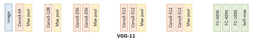
Input Models                           Aligned Models                  Output Model

Figure 1: Model Fusion procedure: The first two steps illustrate how the model A (top) gets aligned
with respect to model B (bottom). The alignment here is reflected by the ordering of the node colors
in a layer. Once each layer has been aligned, the model parameters get averaged (shown by the +) to
yield a fused model at the end.

But in practice, it is more likely to have soft correspondences between the neurons of the two models
for a given layer, especially if their number is not the same across the two models. This is where
optimal transport comes in and provides us a soft-alignment matrix in the form of the transport map T .
In other words, the alignment problem can be rephrased as optimally transporting the neurons in a
given layer of model A to the neurons in the same layer of model B.

General procedure. Let us assume we are at some layer ` and that neurons in the previous layers
have already been aligned. Then, we
                                  define probability measures
                                                                 over neurons in this layer for the
two models as, µ(`) = α(`) , X[`] and ν (`) = β (`) , Y [`] , where X, Y are the measure supports.
Next, we use uniform distributions to initialize the histogram (or probability mass values) for
each layer. Although we note that it is possible to additionally use other measures of neuron
importance [19, 20], but we leave it for a future work. In particular, if the size of layer ` of models A
and B is denoted by n(`) , m(`) respectively, we get α(`) ← 1n(`) /n(`) , β (`) ← 1m(`) /m(`) .
Now, in terms of the alignment procedure, we first align the incoming edge weights for the current
layer `. This can be done by post-multiplying with the previous layer transport matrix T (`−1) ,
normalized appropriately via the inverse of the corresponding column marginals β (`−1) :

                                c (`, `−1) ← W (`, `−1) T (`−1) diag 1/β (`−1) .

                                WA            A                                                        (2)

This update can be interpreted as follows: the matrix T (`−1) diag β −(`−1) has m(`−1) columns in

                                               (`, `−1)
the simplex Σn(`−1) , thus post-multiplying WA          with it will produce a convex combination of
                (`, `−1)
the points in WA         with weights defined by the optimal transport map T (`−1) .
Once this has been done, we focus on aligning the neurons in this layer ` of the two models.
Let us assume, we have a suitable ground metric DS (which we discuss in the sections ahead).
Then we compute the optimal transport map T (`) between the measures µ(`) , ν (`) for layer `, i.e.,
T (`) , W2 ← OT(µ(`) , ν (`) , DS ), where W2 denotes the obtained Wasserstein-distance. Now, we
use this transport map T (`) to align the neurons (more precisely the weights) of the first model (A)
with respect to the second (B),


                                 f (`, `−1) ← T (`) > diag        1      c (`, `−1) .
                                 WA                                     W A                            (3)
                                                                 β (`)

We will refer to model A’s weights, W   f (`, `−1) , as those aligned with respect to model B. Hence, with
                                          A
this alignment in place, we can average the weights of two layers to obtain the fused weight matrix
   (`, `−1)
WF          , as in Eq. (4). We carry out this procedure over all the layers sequentially.
                                   (`, `−1)         f (`, `−1) + W (`, `−1) .
                                            ← 12 W

                                WF                     A            B                                  (4)

                                                       4
Note that, since the input layer is ordered identically for both models, we start the alignment from
second layer onwards. Additionally, the order of neurons for the very last layer, i.e., in the output
layer, again is identical. Thus, the (scaled) transport map at the last layer will be equal to the identity.
Extension to multiple models. The key idea is to begin with an estimate M cF of the fused model,
then align all the given models with respect to it, and finally return the average of these aligned
weights as the final weights for the fused model. For the two model case, this is equivalent to the
procedure we discussed above when the fused model is initialized to model B, i.e., M cF ← MB .
Because, aligning model B with this estimate of the fused model will yield a (scaled) transport map
equal to the identity. And then, Eq. (4) will amount to returning the average of the aligned weights.
Alignment strategies. Now, we discuss how to design the ground metric DS between the inter-
model neurons. Hence, we branch out into the following two strategies to G ET S UPPORT:
(a) Activation-based alignment (acts): In this variant, we run inference over a set of m samples,
S = {x}m i=1 and store the activations for all neurons in the model. Thus, we consider the neuron
activations, concatenated over the samples into a vector, as the support of the measures, and we
denote it as Xk ← ACTS Mk (S) , Y ← ACTS MF (S) . Then the neurons across the two models
are considered to be similar if they produce similar activation outputs for the given set of samples. We
measure this by computing the Euclidean distance between the resulting vector of activations. This
serves as the ground metric for optimal transport computations. In practice, we use the pre-activations.
(b) Weight-based alignment (wts): Here, we consider that the support of each neuron is given by
the weights of the incoming edges (stacked in a vector). Thus, a neuron can be thought as being
represented by the row corresponding to it in the weight matrix. So, the support of the measures
in such an alignment type is given by, Xk [`] ← Wc (`, `−1) , Y [`] ← Wc (`, `−1) . The reasoning for
k F
such a choice stems from the neuron activation at a particular layer being calculated as the inner
product between this weight vector and the previous layer output. The ground metric then used
for OT computations is again the Euclidean distance between weight vectors corresponding to the
neurons p of MA and q of MB (see LINE 12 of Algorithm 2). Besides this difference of employing
the actual weights in the ground metric (LINE 6, 10), rest of the procedure remains identical.
Lastly, the overall procedure is summarized in Algorithm 2 ahead.
4.1 Discussion
Pros and cons of alignment type. An advantage of the weight-based alignment is that it is inde-
pendent of the dataset samples, making it useful in privacy-constrained scenarios. On the flip side,
the activation-based alignment only needs unlabeled data, and an interesting prospect for a future
study would be to utilize synthetic data. But, activation-based alignment may help tailor the fusion to
certain desired kinds of classes or domains. Fusion results for both are nevertheless quite similar (c.f.
Table S2).
Combinatorial hardness of the ideal procedure. In principle, we should actually search over the
space of permutation matrices, jointly across all the layers. But this would be computationally
intractable for models such as deep neural networks, and thus we fuse in a layer-wise manner and in
a way have a greedy procedure.
# of samples used for activation-based alignment. We typically consider a mini-batch of ∼ 100 to
400 samples for these experiments. Table S2 in the Appendix, shows that effect of increasing this
mini-batch size on the fusion performance and we find that even as few as 25 samples are enough to
outperform vanilla averaging.
Exact OT and runtime efficiency: Our fusion procedure is efficient enough for the deep neural
networks considered here (VGG11, R ES N ET 18), so we primarily utilize exact OT solvers. While the
runtime of exact OT is roughly cubic in the cardinality of the measure supports, it is not an issue for
us as this cardinality (which amounts to the network width) is ≤ 600 for these networks. In general,
modern-day neural networks are typically deeper than wide. To give a concrete estimate, the time
taken to fuse six VGG11 models is ≈ 15 seconds on 1 Nvidia V100 GPU (c.f. Section S2.4 for more
details). It is possible to further improve the runtime by adopting the entropy-regularized OT [21],
but this looses slightly in terms of test accuracy compared to exact OT (c.f. Table S4).
5Algorithm 1: Model Fusion (with ψ = {‘acts’, ‘wts’}−alignment)
1: input: Trained models {Mk }K
k=1 and initial estimate of the fused model MF
c
2: output: Fused model MF with weights WF
(`)
3: notation: For model Mk , size of the layer ` is written as nk , and the weight matrix between the layer `
(`, `−1)
and ` − 1 is denoted as Wk . Neuron support tensors are given by Xk , Y .
(1) (1)
4: initialize: The size of input layer nk ← m(1) for all k ∈ [K]; so αk = β (1) ← 1m(1) /m(1) and
(1)
the transport map is defined as Tk ← diag(β (1) ) Im(1) ×m(1) .
5: for each layer ` = 2, . . . , L do
6: β (`) , Y [`] ← 1m(`) /m(`) , G ET S UPPORT(McF , ψ, `)
ν (`) ← β (`) , Y [`]
7: . Define probability measure for initial fused model M
cF
8: for each model k = 1, . . . , K do
c (`, `−1) (`, `−1) (`−1) 1
9: W k ← Wk Tk diag β (`−1)
. Align incoming edges for Mk
(`) (`)
10: αk , Xk [`] ← 1n(`) /nk , G ET S UPPORT(Mk , ψ, `)
k
(`) (`)
11: µk ← αk , Xk [`] . Define probability measure for model Mk
(`)
12: DS [p, q] ← kXk [`][p] − Y [`][q]k2 , ∀ p ∈[n(`)
k
], q ∈[m(`) ] . Form ground metric
(`) (`) (`) (`)
← OT µk , ν (`) , DS
13: Tk , W2 . Compute OT map and distance
f (`, `−1) (`) > 1 (`, `−1)
14: Wk ←T diag (`) Wβ
c
k . Align model Mk neurons
15: end for
(`, `−1) 1
PK f (`, `−1)
16: WF ← K k=1 Wk . Average model weights
17: end for
5 Experiments
Outline. We first present our results for one-shot fusion when the models are trained on different
data distributions. Next, in Section 5.2, we consider (one-shot) fusion in the case when model sizes
are different (i.e., unequal layer widths to be precise). In fact, this aspect facilitates a new tool that
can be applied in ways not possible with vanilla averaging. Further on, we focus on the use-case of
obtaining an efficient replacement for ensembling models in Section 5.3. Lastly, in Section 5.4 we
present fusion in the teacher-student setting, and compare OT fusion and distillation in that context.
Empirical Details. We test our model fusion approach on standard image classification datasets,
like CIFAR10 with commonly used convolutional neural networks (CNNs) such as VGG11 [22]
and residual networks like ResNet18 [23]; and on MNIST, we use a fully connected network with 3
hidden layers of size 400, 200, 100, which we refer to as MLPN ET. As baselines, we mention the
performance of ‘prediction’ ensembling and ‘vanilla’ averaging, besides that of individual models.
Prediction ensembling refers to keeping all the models and averaging their predictions (output layer
scores), and thus reflects in a way the ideal (but unrealistic) performance that we can hope to achieve
when fusing into a single model. Vanilla averaging denotes the direct averaging of parameters. All
the performance scores are test accuracies. Full experimental details are provided in Appendix S2.1.
5.1 Fusion in the setting of heterogeneous data and tasks
We first consider the setting of merging two models A and B, but assume that model A has some
special skill or knowledge (say, recognizing an object) which B does not possess. However, B is
overall more powerful across the remaining set of skills in comparison to A. The goal of fusion now
is to obtain a single model that can gain from the strength of B on overall skills and also acquire the
specialized skill possessed by A. Such a scenario can arise e.g. in reinforcement learning where these
models are agents that have had different training episodes so far. Another possible use case lies in
federated learning [24], where model A is a client application that has been trained to perform well
6(a) Different initialization (b) Same initialization
Figure 2: One-shot skill transfer performance when the specialist model A and the generalist
model B are fused in varying proportions (wB ), for different and same initializations. The OT
avg. (fusion) curve (in magenta) is obtained by activation-based alignment and we plot the mean
performance over 5 seeds along with the error bars for standard deviation. No retraining is done here.
on certain tasks (like personalized keyword prediction) and model B is the server that typically has a
strong skill set for a range of tasks (general language model).
The natural constraints in such scenarios are (a) ensuring privacy and (b) minimization communication
frequency. This implies that the training examples can not be shared between A and B to respect
privacy and a one-shot knowledge transfer is ideally desired, which eliminates e.g., joint training.
At a very abstract level, these scenarios are representative of aggregating models that have been
trained on non-i.i.d data distributions. To simulate a heterogeneous data-split, we consider the
MNIST digit classification task with MLPN ET models, where the unique skill possessed by model A
corresponds to recognizing one particular ‘personalized’ label (say 4), which is unknown to B. Model
B contains 90% of the remaining training set (i.e., excluding the label 4), while A has the other 10%.
Both are trained on their portions of the data for 10 epochs , and other training settings are identical.
Figure 2 illustrates the results for fusing models A and B (in different proportions), both when
they have different parameter initializations or when they share the same initialization. OT fusion 1
significantly outperforms the vanilla averaging of their parameters in terms of the overall test accuracy
in both the cases, and also improves over the individual models. E.g., in Figure 2(a), where the
individual models obtain 89.78% and 87.35% accuracy respectively on the overall (global) test set,
OT avg. achieves the best overall test set accuracy of 93.11%. Thus, confirming the successful skill
transfer from both parent models, without the need for any retraining.
Our obtained results are robust to other scenarios when (i) some other label (say 6) serves as the
special skill and (ii) the % of remaining data split is different. These results are collected in the
Appendix S6, where in addition we also present results without the special label as well.
The case of multiple models. In the above example of two models, one might also consider
maintaining an ensemble, however the associated costs for ensembling become prohibitive as soon
as the numbers of models increases. Take for instance, four models: A, B, C and D, with the
same initialization and assume that A again possessing the knowledge of a special digit (say, 4).
Consider that the rest of the data is divided as 10%, 30%, 50%, 10%. Now training in the similar
setting as before, these models end up getting (global) test accuracies of 87.7%, 86.5%, 87.0%, 83.5%
respectively. Ensembling the predictions yields 95.0% while vanilla averaging obtains 80.6%. In
contrast, OT averaging results in 93.6% test accuracy (≈ 6% gain over the best individual model),
while being 4× more efficient than ensembling. Further details can be found in the Appendix S8.
5.2 Fusing different sized models
An advantage of our OT-based fusion is that it allows the layer widths to be different for each input
model. Here, our procedure first identifies which weights of the bigger model should be mapped to
the smaller model (via the transport map), and then averages the aligned models (now both of the
size of the smaller one). We can thus combine the parameters of a bigger network into a smaller one,
and vice versa, allowing new use-cases in (a) model compression and (b) federated learning.
1
Only the receiver A’s own examples are used for computing the activations, avoiding the sharing of data.
7(a) Post-processing tool for structured prun-
ing. Structured pruning [25–27] is an ap-
proach to model compression that aims to re-
move entire neurons or channels, resulting in
an out-of-the-box reduction in inference costs,
while affecting the performance minimally. A
widely effective method for CNNs is to remove
the filters with smallest `1 norm [25]. Our key
idea in this context is to fuse the original dense
network into the pruned network, instead of just
throwing it away.
Figure 3 shows the gain in test accuracy on CI-
FAR10 by carrying out OT fusion procedure Figure 3: Post-processing for structured prun-
(with weight-based alignment) when different ing: Fusing the initial dense VGG11 model into
convolutional layers of VGG11 are pruned to the pruned model helps test accuracy of the pruned
increasing amounts. For all the layers, we con- model on CIFAR10.
sistently obtain a significant improvement in per-
formance, and ≈ 10% or more gain in the high
sparsity regime. We also observe similar improvements other layers as well as when multiple (or all)
layers are pruned simultaneously (c.f. Appendix S9).
Further, these gains are also significant when measured with respect to the overall sparsity obtained
in the model. E.g., structured pruning the CONV _8 to 90% results in a net sparsity of 23% in the
model. After this pruning, the accuracy of the model drops from 90.3% to 81.5%, and on applying
OT fusion, the performances recovers to 89.4%. As another example take CONV _7, where after
structured pruning to 80%, OT fusion improves the performance of the pruned model from 87.6% to
90.1% while achieving an overall sparsity of 41% in the network (see S9).
Our goal here is not to propose a method for structured pruning, but rather a post-processing tool
that can help regain the drop in performance due to pruning. These results are thus independent of
the pruning algorithm used, and e.g., Appendix S9 shows similar gains when the filters are pruned
based on `2 norm or even randomly. Overall, OT fusion offers a completely data-free approach to
improving the performance of the pruned model, which can be handy in the limited data regime or
when retraining is prohibitive.
(b) Adapting the size of client and server-side mod-
els in federated learning. Given the huge sizes of
contemporary neural networks, it is evident that we
will not able to fit the same sized model on a client
device as would be possible on the server. However,
this might come at the cost of reduced performance.
Further, the resource constraints might be fairly varied
even amongst the clients devices, thus necessitating the
flexibility to adapt the model sizes.
We consider a similar formulation, as in the one-shot
knowledge transfer setting from Section 5.1, except
that now the model B has twice the layer widths as
compared to the corresponding layers of model A. Figure 4: One-shot skill transfer for dif-
Vanilla averaging of parameters, a core component ferent sized models: Results of fusing the
of the widely prevalent FedAvg algorithm [24], gets small client model A into the larger server
ruled out in such a setting. Figure 4 shows how OT model B, for varying proportions wB in
fusion/average can still lead to a successful knowledge which they are fused. See Appendix S7
transfer between the given models. for more details.
5.3 Fusion for efficient ensembling
In this section, our goal is to obtain a single model which can serve as a proxy for an ensemble
of models, even if it comes at a slight decrease in performance relative to the ensemble, for future
8efficiency. Specifically, here we investigate how much can be gained by fusing multiple models that
differ only in their parameter initializations (i.e., seeds). This means that models are trained on the
same data, so unlike in Section 5.1 with a heterogeneous data-split, the gain here might be limited.
We study this in context of deep networks such as VGG11 and R ES N ET 18 which have been trained
to convergence on CIFAR10. As a first step, we consider the setting when we are given just two
models, the results for which are present in Table 1. We observe that vanilla averaging absolutely fails
in this case, and is 3-5× worse than OT averaging, in case of R ES N ET 18 and VGG11 respectively.
OT average, however, does not yet improve over the individual models. This can be attributed to the
combinatorial hardness of the underlying alignment problem, and the greedy nature of our algorithm
as mentioned before. As a simple but effective remedy, we consider finetuning (i.e., retraining) from
the fused or averaged models. Retraining helps for both vanilla and OT averaging, but in comparison,
the OT averaging results in a better score for both the cases as shown in Table 1. E.g., for R ES N ET 18,
OT avg. + finetuning gets almost as good as prediction ensembling on test accuracy.
The finetuning scores for vanilla and
OT averaging correspond to their best DATASET + P REDICTION VANILLA OT F INETUNING
MA MB
obtained results, when retrained with M ODEL AVG . AVG . AVG . VANILLA OT
several finetuning learning rate sched- CIFAR10 + 90.31 90.50 91.34 17.02 85.98 90.39 90.73
ules for a total of 100 and 120 epochs VGG11 1× 1× 2× 2× 2× 2×
in case of VGG11and R ES N ET 18 re- CIFAR10 + 93.11 93.20 93.89 18.49 77.00 93.49 93.78
spectively. We also considered fine- R ES N ET 18 1× 1× 2× 2× 2× 2×
tuning the individual models across
these various hyperparameter settings Table 1: Results for fusing convolutional & residual networks,
(which of course will be infeasible in along with the effect of finetuning the fused models, on CIFAR10.
The number below the test accuracies indicate the factor by which a
practice), but the best accuracy mus- fusion technique is efficient over maintaining all the given models.
tered via this attempt for R ES N ET 18
was 93.51, in comparison to 93.78 for
OT avg. + finetuning. See Appendix S4 and S5 for detailed results and typical retraining curves.
More than 2 models. Now, we discuss the case of more than two models, where the savings in
efficiency relative to the ensemble are even higher. As before, we take the case of VGG11 on
CIFAR10, but now consider four and six such models that have been trained to convergence, each
trained from a different parameter initialization. Table 2 shows the results for this case. We find that
the performance of vanilla averaging degrades to close-to-random performance, and interestingly
even fails to retrain, despite trying various learning rate and schedule hyperparameters. In contrast,
OT average performs significantly better even without retraining, and can be easily retrained to
achieve a significant gain over the individual models.
CIFAR10+ P REDICTION VANILLA OT F INETUNING
I NDIVIDUAL M ODELS
VGG11 AVG . AVG . AVG . VANILLA OT
Accuracy [90.31, 90.50, 90.43, 90.51] 91.77 10.00 73.31 12.40 90.91
Efficiency 1× 1× 4× 4× 4× 4×
Accuracy [90.31, 90.50, 90.43, 90.51, 90.49, 90.40] 91.85 10.00 72.16 11.01 91.06
Efficiency 1× 1× 6× 6× 6× 6×
Table 2: Results of our OT average + finetuning based efficient alternative for ensembling in contrast to vanilla
average + finetuning, for more than two input models (VGG11) with different initializations.
Overall, Tables 1 and 2 show the importance of aligning the networks via OT before averaging.
Further finetuning of the OT fused model, always results in an improvement over the individual
models while being number of models times more efficient than the ensemble.
5.4 Teacher-Student Fusion
We present the results for a setting where we have pre-trained teacher and student networks, and we
would like to transfer the knowledge of the larger teacher network into the smaller student network.
This is essentially reverse of the client-server setting described in Section 5.2, where we fused the
knowledge acquired at the (smaller) client model into the bigger server model. We consider that all
9the hidden layers of the teacher model MA , are a constant ρ× wider than all the hidden layers of
student model MB . Vanilla averaging can not be used due to different sizes of the networks. However,
OT fusion is still applicable, and as a baseline we consider finetuning the model MB .
We experiment with two instances of this (a) on MNIST + MLPN ET, with ρ ∈ {2, 10} and (b)
on CIFAR10 + VGG11, with ρ ∈ {2, 8}, and the results are presented in the Table 3 (results for
MNIST are present in the Table S11). We observe that across all the settings, OT avg. + finetuning
improves over the original model MB , as well as outperforms the finetuning of the model MB , thus
resulting in the desired knowledge transfer from the teacher network.
DATASET + # PARAMS T EACHER S TUDENTS F INETUNING
M ODEL (MA , MB ) MA MB OT AVG . MB OT AVG .
CIFAR10 + (118 M, 32 M) 91.22 90.66 86.73 90.67 90.89
VGG11 (118 M, 3 M ) 91.22 89.38 88.40 89.64 89.85
Table 3: Knowledge transfer from teacher MA into (smaller) student models. The finetuning results
of each method are at their best scores across different finetuning hyperparameters (like, learning rate
schedules). OT avg. has the same number of parameters as MB . Also, here we use activation-based
alignment. Further details can be found in Appendix S12.
Fusion and Distillation. Now, we compare OT fusion, distillation, and their combination, in
context of transferring the knowledge of a large pre-trained teacher network into a smaller student
network. We consider three possibilities for the student model in distillation: (a) randomly initialized
network, (b) smaller pre-trained model MB , and (c) OT fusion (avg.) of the teacher into model MB .
We focus on MNIST + MLPN ET , as it allows us to perform an extensive sweep over the distillation-
based hyperparameters (temperature, loss-weighting factor) for each method. Further, we contrast
these distillation approaches with the baselines of simply finetuning the student models, i.e., finetuning
MB as well as OT avg. model. Results of these experiments are reported in Table 4.
We find that distilling with OT fused model as the student model yields better performance than
initializing randomly or with the pre-trained MB . Further, when averaged across the considered
temperature values = {20, 10, 8, 4, 1}, we observe that distillation of the teacher into random or MB
performs worse than simple OT avg. + finetuning (which also does not require doing such a sweep
that would be prohibitive in case of larger models or datasets). These experiments are discussed in
detail in Appendix S13. An interesting direction for future work would be to use intermediate OT
distances computed during fusion as a means for regularizing or distilling with hidden layers.
T EACHER S TUDENTS F INETUNING D ISTILLATION
MA MB OT AVG . MB OT AVG . R ANDOM MB OT AVG .
98.11 97.84 95.49 98.04 98.19 98.18 98.22 98.30
Mean across distillation temperatures 98.13 98.17 98.26
Table 4: Fusing the bigger teacher model MA to half its size (ρ = 2). Both finetuning and distillation
were run for 60 epochs using SGD with the same hyperparameters. Each entry has been averaged
across 4 seeds.
Hence, this suggests that OT fusion + finetuning can go a long way in an efficient knowledge transfer
from a bigger model into a smaller one, and can be used alongside when distillation is feasible.
6 Conclusion
We show that averaging the weights of models, by first doing a layer-wise (soft) alignment of the
neurons via optimal transport, can serve as a versatile tool for fusing models in various settings. This
results in (a) successful one-shot transfer of knowledge between models without sharing training
data, (b) data free and algorithm independent post-processing tool for structured pruning, (c) and
more generally, combining parameters of different sized models. Lastly, the OT average when
further finetuned, allows for just keeping one model rather than a complete ensemble of models at
inference. Future avenues include application in distributed optimization and continual learning,
10besides extending our current toolkit to fuse models with different number of layers, as well as, fusing
generative models like GANs [12] (where ensembling does not make as much sense). The promising
empirical results of the presented algorithm, thus warrant attention for further use-cases.
Broader Impact
Model fusion is a fundamental building block in machine learning, as a way of direct knowledge
transfer between trained neural networks. Beyond theoretical interest, it can serve a wide range of
concrete applications. For instance, collaborative learning schemes such as federated learning are
of increasing importance for enabling privacy-preserving training of ML models, as well as a better
alignment of each individual’s data ownership with the resulting utility from jointly trained machine
learning models, especially in applications where data is user-provided and privacy sensitive [28].
Here fusion of several models is a key building block to allow several agents to participate in joint
training and knowledge exchange. We propose that a reliable fusion technique can serve as a step
towards more broadly enabling privacy-preserving and efficient collaborative learning.
Acknowledgments
We would like to thank Rémi Flamary, Boris Muzellec, Sebastian Stich and other members of MLO,
as well as the anonymous reviewers for their comments and feedback.
References
[1] Gaspard Monge. Mémoire sur la théorie des déblais et des remblais. Histoire de l’Académie Royale des
Sciences de Paris, 1781.
[2] Leonid V Kantorovich. On the translocation of masses. In Dokl. Akad. Nauk. USSR (NS), volume 37,
pages 199–201, 1942.
[3] Martial Agueh and Guillaume Carlier. Barycenters in the wasserstein space. SIAM Journal on Mathematical
Analysis, 43(2):904–924, 2011.
[4] Marco Cuturi and Arnaud Doucet. Fast computation of wasserstein barycenters. In Eric P. Xing and Tony
Jebara, editors, Proceedings of the 31st International Conference on Machine Learning, volume 32 of
Proceedings of Machine Learning Research, pages 685–693, Bejing, China, 22–24 Jun 2014. PMLR.
[5] Leo Breiman. Bagging predictors. Machine Learning, 24(2):123–140, Aug 1996. ISSN 1573-0565. doi:
10.1023/A:1018054314350. URL https://doi.org/10.1023/A:1018054314350.
[6] David H. Wolpert. Original contribution: Stacked generalization. Neural Netw., 5(2):241–259, February
1992. ISSN 0893-6080. doi: 10.1016/S0893-6080(05)80023-1. URL http://dx.doi.org/10.1016/
S0893-6080(05)80023-1.
[7] Robert E. Schapire. A brief introduction to boosting. In Proceedings of the 16th International Joint
Conference on Artificial Intelligence - Volume 2, IJCAI’99, pages 1401–1406, San Francisco, CA, USA,
1999. Morgan Kaufmann Publishers Inc. URL http://dl.acm.org/citation.cfm?id=1624312.
1624417.
[8] Geoffrey Hinton, Oriol Vinyals, and Jeff Dean. Distilling the knowledge in a neural network. arXiv
preprint arXiv:1503.02531, 2015.
[9] Cristian Buciluǎ, Rich Caruana, and Alexandru Niculescu-Mizil. Model compression. In Proceedings of
the 12th ACM SIGKDD International Conference on Knowledge Discovery and Data Mining, KDD ’06,
pages 535–541, New York, NY, USA, 2006. ACM. ISBN 1-59593-339-5. doi: 10.1145/1150402.1150464.
URL http://doi.acm.org/10.1145/1150402.1150464.
[10] Jürgen Schmidhuber. Learning complex, extended sequences using the principle of history compression.
Neural Computation, 4(2):234–242, 1992.
[11] Zhiqiang Shen, Zhankui He, and Xiangyang Xue. Meal: Multi-model ensemble via adversarial learning,
2018.
[12] Ian Goodfellow, Jean Pouget-Abadie, Mehdi Mirza, Bing Xu, David Warde-Farley, Sherjil Ozair, Aaron
Courville, and Yoshua Bengio. Generative adversarial nets. In Advances in neural information processing
systems, pages 2672–2680, 2014.
11[13] Joshua Smith and Michael Gashler. An investigation of how neural networks learn from the experiences
of peers through periodic weight averaging. In 2017 16th IEEE International Conference on Machine
Learning and Applications (ICMLA), pages 731–736. IEEE, 2017.
[14] Joachim Utans. Weight averaging for neural networks and local resampling schemes. In Proc. AAAI-96
Workshop on Integrating Multiple Learned Models. AAAI Press, pages 133–138, 1996.
[15] Mikhail Iu Leontev, Viktoriia Islenteva, and Sergey V Sukhov. Non-iterative knowledge fusion in deep
convolutional neural networks. arXiv preprint arXiv:1809.09399, 2018.
[16] Sebastian Urban Stich. Local sgd converges fast and communicates little. In ICLR 2019 - International
Conference on Learning Representations, 2019.
[17] Mikhail Yurochkin, Mayank Agarwal, Soumya Ghosh, Kristjan Greenewald, Trong Nghia Hoang, and
Yasaman Khazaeni. Bayesian nonparametric federated learning of neural networks, 2019.
[18] Hongyi Wang, Mikhail Yurochkin, Yuekai Sun, Dimitris Papailiopoulos, and Yasaman Khazaeni. Federated
learning with matched averaging. In International Conference on Learning Representations, 2020. URL
https://openreview.net/forum?id=BkluqlSFDS.
[19] Kedar Dhamdhere, Mukund Sundararajan, and Qiqi Yan. How important is a neuron. In International Con-
ference on Learning Representations, 2019. URL https://openreview.net/forum?id=SylKoo0cKm.
[20] Mukund Sundararajan, Ankur Taly, and Qiqi Yan. Axiomatic attribution for deep networks, 2017.
[21] Marco Cuturi. Sinkhorn distances: Lightspeed computation of optimal transport. In Advances in neural
information processing systems, pages 2292–2300, 2013.
[22] Karen Simonyan and Andrew Zisserman. Very deep convolutional networks for large-scale image recogni-
tion, 2014.
[23] Kaiming He, Xiangyu Zhang, Shaoqing Ren, and Jian Sun. Deep residual learning for image recognition.
2016 IEEE Conference on Computer Vision and Pattern Recognition (CVPR), Jun 2016. doi: 10.1109/cvpr.
2016.90. URL http://dx.doi.org/10.1109/CVPR.2016.90.
[24] H. Brendan McMahan, Eider Moore, Daniel Ramage, Seth Hampson, and Blaise Agüera y Arcas.
Communication-efficient learning of deep networks from decentralized data, 2016.
[25] Hao Li, Asim Kadav, Igor Durdanovic, Hanan Samet, and Hans Peter Graf. Pruning filters for efficient
convnets, 2016.
[26] Pavlo Molchanov, Arun Mallya, Stephen Tyree, Iuri Frosio, and Jan Kautz. Importance estimation for
neural network pruning. In The IEEE Conference on Computer Vision and Pattern Recognition (CVPR),
June 2019.
[27] Sajid Anwar, Kyuyeon Hwang, and Wonyong Sung. Structured pruning of deep convolutional neural
networks. J. Emerg. Technol. Comput. Syst., 13(3), February 2017. ISSN 1550-4832. doi: 10.1145/3005348.
URL https://doi.org/10.1145/3005348.
[28] Peter Kairouz, H Brendan McMahan, Brendan Avent, Aurélien Bellet, Mehdi Bennis, Arjun Nitin Bhagoji,
Keith Bonawitz, Zachary Charles, Graham Cormode, Rachel Cummings, et al. Advances and open
problems in federated learning. arXiv preprint arXiv:1912.04977, 2019.
[29] Ari S. Morcos, Maithra Raghu, and Samy Bengio. Insights on representational similarity in neural networks
with canonical correlation, 2018.
[30] Sira Ferradans, Nicolas Papadakis, Julien Rabin, Gabriel Peyré, and Jean-François Aujol. Regularized
discrete optimal transport. Scale Space and Variational Methods in Computer Vision, page 428–439,
2013. ISSN 1611-3349. doi: 10.1007/978-3-642-38267-3_36. URL http://dx.doi.org/10.1007/
978-3-642-38267-3_36.
[31] L. Ambrosio, Nicola Gigli, and Giuseppe Savare. Gradient flows: in metric spaces and in the space of
probability measures. 2006. URL https://www.springer.com/gp/book/9783764387211.
[32] Song Mei, Theodor Misiakiewicz, and Andrea Montanari. Mean-field theory of two-layers neural networks:
dimension-free bounds and kernel limit, 2019.
12Appendix
S1 Model Fusion Algorithm
Algorithm 2: Model Fusion (with ψ = {‘acts’, ‘wts’}−alignment)
1: input: Trained models {Mk }K
k=1 and initial estimate of the fused model MF
c
2: output: Fused model MF with weights WF
(`)
3: notation: For model Mk , size of the layer ` is written as nk , and the weight matrix between the layer `
(`, `−1)
and ` − 1 is denoted as Wk . Neuron support tensors are given by Xk , Y .
(1) (1)
4: initialize: The size of input layer nk ← m(1) for all k ∈ [K]; so αk = β (1) ← 1m(1) /m(1) and
(1)
the transport map is defined as Tk ← diag(β (1) ) Im(1) ×m(1) .
5: for each layer ` = 2, . . . , L do
6: β (`) , Y [`] ← 1m(`) /m(`) , G ET S UPPORT(McF , ψ, `)
ν (`) (`)
7: ← β , Y [`] . Define probability measure for initial fused model M
cF
8: for each model k = 1, . . . , K do
c (`, `−1) (`, `−1) (`−1) 1
9: W k ← Wk Tk diag β (`−1)
. Align incoming edges for Mk
(`) (`)
10: αk , Xk [`] ← 1n(`) /nk ,
G ET S UPPORT(Mk , ψ, `)
k
(`) (`)
11: µk ← αk , Xk [`] . Define probability measure for model Mk
(`)
12: DS [p, q] ← kXk [`][p] − Y [`][q]k2 , ∀ p ∈[n(`)
k
], q ∈[m(`) ] . Form ground metric
(`) (`) (`) (`) (`)
13: Tk , W2 ← OT µk , ν , DS . Compute OT map and distance
f (`, `−1) (`) > 1 (`, `−1)
14: Wk ←T diag (`) β
W
c
k . Align model Mk neurons
15: end for
(`, `−1) 1
PK f (`, `−1)
16: WF ← K k=1 Wk . Average model weights
17: end for
Before going further, note that our code can be found under the following link
https://github.com/modelfusion/otfusion.
13S2 Technical specifications
S2.1 Experimental Details
VGG11 training details. It is trained by SGD for 300 epochs with an initial learning rate of
0.05, which gets decayed by a factor of 2 after every 30 epochs. Momentum = 0.9 and weight
decay = 0.0005. The batch size used is 128. Checkpointing is done after every epoch and the best
performing checkpoint in terms of test accuracy is used as the individual model. The block diagram
of VGG11 architecture is shown below for reference.
Figure S1: Block diagram of the VGG11 architecture. Adapted from https://bit.ly/2ksX5Eq.
MLPN ET training details. This is also trained by SGD at a constant learning rate of 0.01 and
momentum = 0.5. The batch size used is 64.
R ES N ET 18 training details. Again, we use SGD as the optimizer, with an initial learning rate of
0.1, which gets decayed by a factor of 10 at epochs {150, 250}. In total, we train for 300 epochs
and similar to the VGG11 setting we use the best performing checkpoint as the individual model.
Other than that, momentum = 0.9, weight decay = 0.0001, and batch size = 256. We skip the batch
normalization for the current experiments, however, it can possibly be handled by simply multiplying
the batch normalization parameters in a layer by the obtained transport map while aligning the
neurons.
Other details. Pre-activations. The results for the activation-based alignment experiments are
based on pre-activation values, which were generally found to perform slightly better than post-
activation values.
Regularization. The regularization constant used for the activation-based alignment results in Table
S2 is 0.05.
Common details. The bias of a neuron is set to zero in all of the experiments. It is possible to handle
it as a regular weight by keeping the corresponding input as 1, but we leave that for future work.
S2.2 Combining weights and activations for alignment
The output activation of a neuron over input examples gives a good signal about the presence of
features in which the neuron gets activated. Hence, one way to combine this information in the above
variant with weight-based alignment is to use them in the probability mass values.
In particular, we can take a mini-batch of samples and store the activations of all the neurons. Then
we can use the mean activation as a measure of a neuron’s significance. But it might be that some
neurons produce very high activations (in absolute terms) irrespective of the kind of input examples.
Hence, it might make sense to also look at the standard deviation of activations. Thus, one can
combine both these factors into an importance weight for the neuron as follows:
importancek [2, · · · , L] = Mk ([x1 , · · · , xd ]) σ(Mk ([x1 , · · · , xd ])) (5)
Here, Mk denotes the k th model into which we pass the inputs [x1 , · · · , xd ], M denotes the mean,
σ(.) denotes the standard deviation and denotes the elementwise product. Thus, we can now set
(l)
the probability mass values bk ∝ importancek [l], and the rest of the algorithm remains the same.
14S2.3 Optimal Transport
We make use of the Python Optimal Transport (POT)S1 for performing the computation of Wasserstein
distances and barycenters on CPU. These can also be implemented on the GPU to further boost the
efficiency, although it suffices to run on CPU for now, as evident from the timings below.
S2.4 Timing information
The following timing benchmarks are done on 1 Nvidia V100 GPU. The time taken to average two
MLPN ET models for MNIST is ≈ 3 seconds. For averaging VGG11 models on CIFAR10, it takes
about ≈ 5 seconds. While in case of R ES N ET 18 on CIFAR10, it takes ≈ 7 seconds. These numbers
are for the activation-based alignment, and also include the time taken to compute the activations
over the mini-batch of examples.
The weight-based alignment can be faster as it does not need to compute the activations. For instance,
when weight-based alignment is employed to average two VGG11 models on CIFAR10, it takes ≈
2.5 seconds.
S3 Ablation studies
S3.1 Aggregation performance as training progresses
We compare the performance of averaged models at various points during the course of training
the individual models (for the setting of MLPNet on MNIST). We notice that in the early stages
of training, vanilla averaging performs even worse, which is not the case for OT averaging. The
corresponding Figure S2 and Table S1 can be found in Section S3.1 of the Appendix. Overall, we see
OT averaging outperforms vanilla averaging by a large margin, thus pointing towards the benefit of
aligning the neurons via optimal transport.
100
90
80
70
60
model_1 accuracy
model_2 accuracy
prediction accuracy
50 vanilla accuracy
structure-aware (act) accuracy
2.5 5.0 7.5 10.0 12.5 15.0 17.5 20.0
Figure S2: Illustrates the performance of various aggregation methods as training proceeds, for
(MNIST, MLPN ET). The plots correspond to the results reported in Table S1. The activation-based
alignment of the OT average (labelled as structure-aware accuracy in the figure) is used based on
m = 200 samples.
S3.2 Transport map for the output layer.
Since our algorithm runs until the output layer, we inspect the alignment computed for the last output
layer. We find that the ratio of the trace to the sum for this last transport map is ≈ 1, indicating
accurate alignment as the ordering of output units is the same across models.
S1
http://pot.readthedocs.io/en/stable/
15E POCH M ODEL A M ODEL B P REDICTION AVG . VANILLA AVG . OT AVG .
01 92.03 92.40 92.50 47.39 87.10
02 94.39 94.43 94.79 52.28 91.72
05 96.83 96.58 96.93 58.96 95.30
07 97.36 97.34 97.48 68.76 95.26
10 97.72 97.75 97.88 73.84 95.92
15 97.91 97.97 98.11 73.55 95.60
20 98.11 98.04 98.13 73.91 95.31
Table S1: Activation-based alignment (MNIST, MLPNet): Comparison of performance when
ensembled after different training epochs. The # samples used for activation-based alignment,
m = 50. The corresponding plot for this table is illustrated in Figure S2.
S3.3 Effect of mini-batch size needed for activation-based mode
Here, the individual models used are MLPN ET’s which have been trained for 10 epochs on MNIST.
They differ only in their seeds and thus in the initialization of the parameters alone. We ensemble the
final checkpoint of these models via OT averaging and the baseline methods.
P REDICTION VANILLA OT AVG . (S INKHORN ) MA ALIGNED
MA MB m
AVG . AVG . Accuracy (mean ± stdev)
(a) Activation-based Alignment
2 24.80 ± 6.93 20.08 ± 2.42
10 75.04 ± 11.35 88.18 ± 8.45
25 90.95 ± 3.98 95.36 ± 0.96
97.72 97.75 97.88 73.84
50 93.47 ± 1.69 96.04 ± 0.59
100 95.40 ± 0.52 97.05 ± 0.17
200 95.78 ± 0.52 97.01 ± 0.16
(b) Weight-based Alignment
97.72 97.75 97.88 73.84 — 95.66 96.32
Table S2: One-shot averaging for (MNIST, MLPNet) with Sinkhorn and regularization = 0.05:
Results showing the performance (i.e., test classification accuracy (in %)) of the OT averaging in
contrast to the baseline methods. The last column refers to the aligned model A which gets (vanilla)
averaged with model B, giving rise to our OT averaged model. m is the size of mini-batch over which
activations are computed.
S3.4 Effect of regularization
The results for activation-based alignment presented in the Table S2 above use the regularization
constant λ = 0.05. Below, we also show the results with a higher regularization constant λ = 0.1. As
expected, we find that using a lower value of regularization constant leads to better results in general,
since it better approximates OT.
OT AVG . MA aligned
MA MB P REDICTION VANILLA m
Accuracy (mean ± stdev)
2 25.05 ± 7.22 19.42 ± 2.28
10 72.86 ± 11.93 74.35 ± 14.40
25 89.49 ± 5.21 90.88 ± 4.91
97.72 97.75 97.88 73.84
50 92.88 ± 2.03 94.54 ± 1.36
100 95.14 ± 0.49 96.42 ± 0.39
200 95.70 ± 0.54 96.63 ± 0.23
Table S3: Activation-based alignment (MNIST, MLPNet) with Sinkhorn and regularization = 0.1:
Results showing the performance (i.e., test classification accuracy ) of the averaged and aligned
models of OT based averaging in contrast to vanilla averaging of weights as well as the prediction
based ensembling. m denotes the number of samples over which activations are computed, i.e., the
mini-batch size.
16You can also read