SCALING SYMBOLIC METHODS USING GRADIENTS FOR NEURAL MODEL EXPLANATION
←
→
Page content transcription
If your browser does not render page correctly, please read the page content below
Under review as a conference paper at ICLR 2021

S CALING S YMBOLIC M ETHODS USING G RADIENTS
FOR N EURAL M ODEL E XPLANATION

 Anonymous authors
 Paper under double-blind review

                                              A BSTRACT

         Symbolic techniques based on Satisfiability Modulo Theory (SMT) solvers have
         been proposed for analyzing and verifying neural network properties, but their
         usage has been fairly limited owing to their poor scalability with larger networks.
         In this work, we propose a technique for combining gradient-based methods with
         symbolic techniques to scale such analyses and demonstrate its application for
         model explanation. In particular, we apply this technique to identify minimal
         regions in an input that are most relevant for a neural network’s prediction. Our
         approach uses gradient information (based on Integrated Gradients) to focus on a
         subset of neurons in the first layer, which allows our technique to scale to large
         networks. The corresponding SMT constraints encode the minimal input mask
         discovery problem such that after masking the input, the activations of the selected
         neurons are still above a threshold. After solving for the minimal masks, our
         approach scores the mask regions to generate a relative ordering of the features
         within the mask. This produces a saliency map which explains “where a model is
         looking” when making a prediction. We evaluate our technique on three datasets -
         MNIST, ImageNet, and Beer Reviews, and demonstrate both quantitatively and
         qualitatively that the regions generated by our approach are sparser and achieve
         higher saliency scores compared to the gradient-based methods alone.

1    I NTRODUCTION

Satisfiability Modulo Theory (SMT) solvers (Barrett & Tinelli, 2018) are routinely used for symbolic
modeling and verifying correctness of software programs (Srivastava et al., 2009), and more recently
they have also been used for verifying properties of deep neural networks (Katz et al., 2017). SMT
Solvers in their current form are difficult to scale to large networks. Model explanation is one
such domain where SMT solvers have been used but they are limited to very small sized networks
(Gopinath et al., 2019; Ignatiev et al., 2019). The goal of our work is to address the issue of scalability
of SMT solvers by using gradient information, thus enabling their use for different applications. In
this work, we present a new application of SMT solvers for explaining neural network decisions.
Model explanation can be viewed as identifying a minimal set of features in a given input that
is critical to a model’s prediction (Carter et al., 2018; Macdonald et al., 2019). Such a problem
formulation for identifying a minimal set lends itself to the use of SMT solvers for this task. We can
encode a neural network using real arithmetic (Katz et al., 2017) and use an SMT solver to optimize
over the constraints to identify a minimal set of inputs that can explain the prediction. However, there
are two key challenges in this approach. First, we cannot generate reliable explanations based on
final model prediction as the minimal input is typically out of distribution. Second, solving such a
formulation is challenging for SMT solvers as the decision procedures for solving these constraints
have exponential complexity, and is further exacerbated by the large number of parameters in typical
neural network models. Thus, previous approaches for SMT-based analysis of neural networks have
been quite limited, and have only been able to scale to networks with few thousands of parameters.
To solve these challenges, instead of doing minimization by encoding the entire network, our approach
takes advantage of the gradient information, specifically Integrated Gradients (IG) (Sundararajan
et al., 2017), in lieu of encoding the deeper layers, and encodes a much simpler set of linear constraints
pertaining to the layer closest to the input. We encode the mathematical equations of a neural network
as SMT constraints using the theory of Linear Real Arithmetic (LRA), and use z3 solver (Bjørner

                                                    1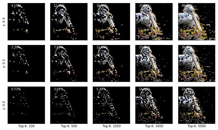
Under review as a conference paper at ICLR 2021

et al., 2015) as it additionally supports optimization constraints such as minimization. The SMT
solver then finds a minimal subset (of input features) by performing minimization on these equations.
Thus, our approach, which we refer to as SMUG, is able to scale Symbolic Methods Using Gradient
information while still providing a faithful explanation of the neural network’s decision.
SMUG is built on two properties. First, based on the target prediction, SMUG uses gradient
information propagated from the deeper layers to identify neurons that are important in the first layer,
and only encodes those. For this, we use IG (Sundararajan et al., 2017) instead of relying on gradients
alone. Second, for the optimization, a set of input pixels are determined to be relevant for prediction
if they are able to activate the neurons deemed important, and maintain a fraction of their activation
as the original (full) input image. Empirically, we observe good performance on visual and text
classification tasks.
We evaluate SMUG on three datasets: MNIST (LeCun et al., 2010), ImageNet (Deng et al., 2009),
and Beer Reviews (McAuley et al., 2012). We show that we can fully encode the minimal feature
identification problem for a small feedforward network (without gradient-based neuron selection)
for MNIST, but this full SMT encoding scales poorly for even intermediate sized networks. On
ImageNet, we observe that our method performs better than Integrated Gradients (Sundararajan et al.,
2017) and several strong baselines. Additionally, we observe that our approach finds significantly
sparser masks (on average 17% of the original image size). Finally, we also show that our technique is
applicable to text models where it performs competitively with other methods including SIS (Carter
et al., 2018) and Integrated Gradients (Sundararajan et al., 2017).
This paper makes the following key contributions:
       • We present a technique (SMUG) to encode the minimal input feature discovery problem for
         neural model explanation using SMT solvers.
       • Our approach uses gradient information to scale SMT-based analysis of neural networks to
         larger models and input features. Further, it also overcomes the issue of choosing a “baseline”
         parameter for Integrated Gradients (Kapishnikov et al., 2019; Sturmfels et al., 2020).
       • We empirically evaluate SMUG on image and text datasets, and show that the minimal
         features identified by it are both quantitatively and qualitatively better than several baselines.

2    R ELATED W ORK
SMT based symbolic techniques have been used for verifying neural network properties (Huang et al.,
2017; Katz et al., 2017). Reluplex (Katz et al., 2017) extends the simplex method to handle ReLU
functions by leveraging its piecewise linear property and presents an iterative procedure for gradual
satisfaction of the constraints. (Huang et al., 2017) proposes a layer-wise analysis using a refinement-
based approach with SMT solvers for verifying the absence of adversarial input perturbations. (Zhang
et al., 2018) present a linear programming (LP) formulation again using the piecewise linear property
of ReLU to find minimal changes to an input to change a network’s classification decisions. (Gopinath
et al., 2019) uses Reluplex to learn input properties in the form of convex predicates over neuron
activations, which in turn capture different behaviors of a neural network. While these techniques
have shown promising results, scaling these approaches for larger neural networks and performing
richer analysis based on global input features still remains a challenge.
While the above SMT based techniques focus on verifying properties of deep networks, our work
focuses on applying symbolic techniques to the related task of model explanation, i.e. to say where
a model is “looking”, by solving for the input features responsible for a model’s prediction. Some
explanation techniques are model agnostic (i.e., black-box) while others are back-propagation based.
Model agnostic (black-box) explanation techniques such as SIS, L IME (Alvarez-Melis & Jaakkola,
2018; Carter et al., 2018) have a similar formulation of the problem as ours in the sense that they
perturb the input pixels by masking them and optimize to identify minimal regions affecting the
performance of the model. This formulation can lead to evaluating the model on out of distribution
samples (Hooker et al., 2019) with potential for adversarial attacks (Slack et al., 2020). In contrast,
back-propagation based methods (Bach et al., 2015; Sundararajan et al., 2017; Selvaraju et al., 2016)
examine the gradients of the model with respect to an input instance to determine pixel attribution.
Our work builds on the IG method (Sundararajan et al., 2017). IG integrates gradients along the
“intensity” path where the input (image or text embedding) is scaled from an information-less baseline

                                                    2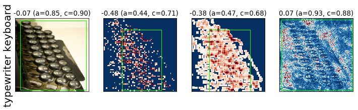
Under review as a conference paper at ICLR 2021

(all zeros input, e.g., all black or random noise image) to a specific instance. This helps the model
determine attribution at the pixel level. In our work, we use IG to determine important nodes in the
first layer (closest to the input). The key improvement of our technique over IG is that, by using IG
only on the first layer and then using SMT solver based solution to determine saliency on the input,
we not only preserve faithfulness, but also overcome the issue of choosing an appropriate baseline
image for IG (Kapishnikov et al., 2019; Sturmfels et al., 2020; Xu et al., 2020).

3     M ETHOD : S CALING S YMBOLIC M ETHODS U SING G RADIENTS (SMUG)

We describe our approach SMUG, which combines attribution based on gradient information with
an SMT-based encoding of the minimal input feature identification problem. We then show how to
generate saliency maps from the predicted boolean mask for image and text applications.

3.1   C HALLENGES WITH ENCODING NEURAL NETWORKS FOR EXPLANATION

Previous works (Katz et al., 2017) have shown it’s possible to use SMT solvers to encode the
semantics of neural networks with specific activation functions, while others (Carter et al., 2018;
Macdonald et al., 2019) have used the idea of minimality to identify importance of inputs in the
context of model explanation. In particular, given a neural network Nθ (θ denotes the parameters), let
X ∈ Rm×n denote an input image with m × n pixels, M ∈ {0, 1}m×n an unknown binary mask,
and Li (·) the output (i.e., activations) of the ith layer. Also, let L|L|−1 (Nθ (X)) denote the logits of
the final layer. Previous works (Carter et al., 2018; Macdonald et al., 2019) have used the following
formulation for explanation.
                   X
             min(      Mij ) : argmax L|L|−1 (Nθ (X)) = argmax L|L|−1 (Nθ (M X))
                   ij

However, there are two key problems with this formulation. First, the masked inputs found by solving
this formulation are typically out of training distribution, so explanation techniques based on model
confidence over a forward pass of the masked inputs (such as the above formulation) no longer
produce reliable explanations. Second, using such a formulation directly with SMT solvers is not
tractable as the number of constraints in the encoding grows linearly with increasing network size
and SMT decision procedure for Non-linear Real Arithmetic is doubly exponential. Thus, when we
apply such an encoding even for a small feed-forward network on MNIST dataset, the SMT solver
does not scale well (Section 4, Appendix. A).

3.2   O UR S OLUTION : C OMBINING G RADIENTS WITH S YMBOLIC E NCODING

Our proposal is to use gradient based attributions to overcome both these issues: 1) as a proxy for
the deeper layers (for scalability), and 2) to identify a subset of neurons in the first layer capturing
information crucial for the model’s prediction, and encode them using SMT which avoids performing
a forward pass on out-of-distribution inputs.
Specifically, we use Integrated Gradients (IG) (Sundararajan et al., 2017) to score the neurons in
order of relevance by treating the first layer activations (L1 ) as an input to the subsequent network.
This assigns an attribution score to each hidden node where a node with a positive score means that
the information captured by that neuron is relevant to the prediction and a node with a negative /
zero score is considered irrelevant. More specifically, suppose F : Ra×b×c → [0, 1]d represents a
deep network and x represents the input. F often refers to the full network (from the input to the
final softmax) but in our case, it refers to the nodes in the network second through the final layer.
a, b, and c refer to the dimensions of the tensor input to the network (analogous to width, height,
and channels) and d is the number of output nodes in the final softmax layer (number of classes).
Integrated gradients are obtained by accumulating the gradients at all points along the straight line
path from an “information-less” baseline x0 to the input x. The information-less baseline in this case
is an all zeros tensor. The path can be parameterized as g(α) = x0 + α · (x − x0 ). IG is then given by
Eq. 1.
                                                    Z 1
                                                  0       ∂F (g(α))
                                 IG(x) = (x − x )                     dα                            (1)
                                                      α=0   ∂g(α)

                                                    3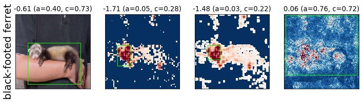
Under review as a conference paper at ICLR 2021

Top-k Neurons. The second key idea of our approach is that we only consider activations with the
highest positive attributions. Empirically, we still observe scaling issues with SMT when considering
all first layer neurons (L1 ) with +ve attributions, so a method for picking a subset of neurons (top-k
attributions) is important for practical application.
With these two ideas, we can now formulate our problem as follows. Let, Dk represent the set of k
important nodes with the highest attributions in IG(Nθ (X)), and γ be a parameter which regulates
how “active” the neurons remain after masking1 .The goal now is to learn a mask M such that:
                     X
                 min(  Mij ) : L1 (Nθ (M           X))t > γ · L1 (Nθ (X))t              ∀t ∈ Dk            (2)
                       ij

IG ensures that the information captured by the neurons in Dk are relevant for the model’s prediction.
Thus, the set of features corresponding to these neurons contributes towards the relevant information.
Let’s denote this set as S. To filter less relevant features from S we introduce a notion of minimization.
Thus, we define "relevant features" as a minimal subset of features in S that causes the nodes in Dk
to remain active. The notion being - if for a masked input the "important nodes" (for the original
input) are active then it means that the information relevant for the prediction of the original image is
contained in the mask. Thus, the mask highlights features relevant for the model’s prediction.

3.3   SMT FORMULATION OF M INIMAL I NPUT M ASK D ISCOVERY P ROBLEM

Given Dk , a set of k neurons with highest positive attributions in IG(Nθ (X)), our goal is to find a
minimal mask such that the activations of these neurons are above some threshold (γ) times their
original activation values. Eq. 3 shows the constraints for a minimal mask. The first set of constraint
specifies that the unknown mask variable M can only have 0 and 1 as possible entries in the matrix.
The second and third set of constraints encode the activation values of the first layer of network with
corresponding masked and original inputs respectively. The fourth set of constraint states that the
activations of these k neurons should be at least γ times the original activation values, and the final
constraint adds the optimization constraint to minimize the sum of all the mask bits. Note that here
we show the formulation for a feedforward network and a input X with 2 channels, but it can be
extended to convolutional networks and an input with 3rd channel as well in a straightforward manner
where the mask variables across the same channel share the same mask variable.
                     ^                                       ^
         ∃M :                (Mij == 0) ∨ (Mij == 1)             om
                                                                  i = (W1 (X        M ) + b1 )i
                1≤i≤m,1≤j≤n                                     ∀i∈D k
                            ^                           ^                      ^                           (3)
                                 oi = (W1 X + b1 )i            om
                                                                i   > γ · oi       minimize(Σij Mij )
                        ∀i∈D k                        ∀i∈D k

3.4   C ONSTRUCTING S ALIENCY M AP FROM B INARY M ASK

The SMT solver generates a minimal binary input mask by solving the constraints shown in Eq. 3.
We further use the attribution scores obtained from IG to assign importance scores to each mask pixel.
A mask variable Mij that is assigned a value of 1 by SMT is assigned a score sij computed as:

                                      α(op )1receptive(op ) (xij )
                                X
                      sij =                                               ∀i, j : Mij = 1                  (4)
                              1≤p≤k

where α(op ) denotes the attribution score assigned by IG for neuron op and the indicator function
denotes that pixel xij is present in the receptive field of op , i.e. it is present in the linear SMT
equation used to compute on . These scores are then used to compute a continuous saliency map for
an input (Appendix. 9). Finally, to amplify the pixel differences for visualization purposes in gray
scale, we scale the non-zero score values between 0.5 and 1.

   1
     This formulation is valid for networks with ReLU activations and would need to be modified for a different
choice of activation such as tanh.

                                                       4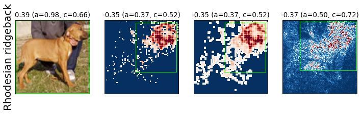
Under review as a conference paper at ICLR 2021

4    E XPERIMENTAL S ETUP
Datasets. We empirically evaluate SMUG on two image datasets, MNIST (LeCun et al., 2010),
and ImageNet (Deng et al., 2009), as well as a text dataset of Beer Reviews from (McAuley et al.,
2012).
MNIST: We use the MNIST dataset to show the scalability of the full network encoding in SMT
(presented in Section 3.1). We use a feedforward model consisting of one hidden layer with 32 nodes
(ReLU activation) and 10 output nodes with sigmoid, one each for 10 digits (0 - 9). For 100 images
chosen randomly from the validation set, the SMT solver could solve the constraint shown in Eq. 6
(returns S AT) for only 41 of the images. For the remaining 59 images, the solver returns U NKNOWN,
which means the given set of constraints was too difficult for the solver to solve.
ImageNet: We use 3304 images (224 × 224) with ground truth bounding boxes from the validation
set of ImageNet. The images for which the model classification was correct and a ground truth
bounding box annotation for the object class was available were chosen. We use the Inception-v1
model from (Szegedy et al., 2015) which classifies images into one of the 1000 ImageNet classes.
Beer Reviews: To evaluate SMUG on a textual task we consider the review rating prediction task
on the Beer Reviews dataset consisting of 70k training examples, 3k validation and 7k test examples.
Additionally, the dataset comes with ground truth annotations where humans provide the rationale
(select words) that correspond to the rating and review. We train a 1D CNN model to predict the
rating for the aroma of the beer on a scale from 0 to 1. This model is identical to the model used in
(Carter et al., 2018) and consists of a convolution layer with 128 kernels followed by a ReLU, a fully
connected layer, and a sigmoid. It achieves a validation mean square error of 0.032.
Metrics. Assessing the quality of the saliency maps, especially binary masks, is challenging. The
change in confidence of the classifier (between the original and masked) image alone may not be
a reliable measure since the masked input could fall out of the training distribution (Hooker et al.,
2019). Instead, we use the metric proposed in (Dabkowski & Gal, 2017) shown in Eq. 5. This metric,
which we term Log Sparsity Confidence difference (LSC) score, first finds the tightest bounding box
that captures the entire mask, then computes confidence on the cropped box resized to the original
image size (we use bilinear interpolation). This not only helps keep images closer to the training
distribution, but also helps evaluate explanations without the need for groundtruth annotations. The
LSC score is computed as:
                       LSC(a, c) = log(ã) − log(c),          ã = max(0.05, a)                      (5)
where a is the fractional area of the rectangular cropped image and c is the confidence of the classifier
for the true label on the cropped image. A saliency map that is compact and allows the model to
still recognize the object would result in a lower LSC score. LSC captures model confidence as
well as compactness of the identified salient regions, both of which are desirable when evaluating an
explanation. The compactness in particular also makes it suitable for evaluating SMT based methods
for the effect of minimization. We adapt LSC to also assess continuous valued saliency maps by,
1) setting a threshold on the continuous valued saliency map to convert them to a binary mask and
2) iterating over multiple thresholds (in steps) to identify the one that results in the best LSC score.
We also report the fraction of images for which the mask generated by a given method is better (i.e.
produces an equal or lower LSC score) than other methods, which we refer to as Win%.
Comparison methods. The final saliency mask for SMUG comes from Eq. 4 (Sec. 3.4). We
compare this to the saliency maps, and bounding boxes from several baselines described below.
SMUGbase is a variant of SMUG that does not peform SMT-based minimization. Here, in Eq. 2,
we simply set Mij = 1 for each pixel xij that is in the receptive fields of the top-k neurons in
the first layer (L1 ) selected by IG. We note here that in case of both SMUG and SMUGbase in the
formulations in Eq. 2 and 3, we set k = 3000, γ = 0 for ImageNet, and k = 100, γ = 0 for text
experiments (this choice is explored more in the supplementary material).
IG corresponds to Integrated Gradients (Sundararajan et al., 2017) with the black image as a baseline.
G RAD C AM (Selvaraju et al., 2017) uses a weighted average of the CNN filters for saliency, with
weights informed by the gradients.
SIS refers to Sufficient Input Subset (Carter et al., 2018), which finds multiple disjoint subsets of
input features (in decreasing order of relevance) which individually allow a confident classification.
SIS did not scale for ImageNet and we only compare against it on the text dataset.

                                                   5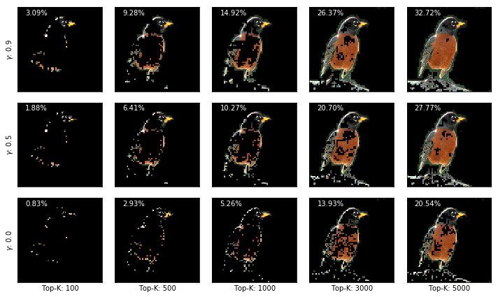
Under review as a conference paper at ICLR 2021

G ROUND T RUTH corresponds to the baseline that uses human annotated bounding box, which
capture the object corresponding to the image label.
M AX B OX denotes maximal mask spanning the entire image.
C ENTER B OX uses a bounding box placed at the center of the image covering half of the image area.
O PT B OX refers to a bounding box that approximtely optimizes for LSC. The saliency metric in Eq. 5
relies on finding a single bounding box for an image. To find a box that directly maximizes the metric,
we first discretize the image into subgrids of 10 × 10 pixels; and then perform a brute force search by
selecting 2 points on the grid (to represent opposite corners of a rectangle) and identify a subgrid
with the best score.

5      R ESULTS
5.1     I MAGE N ET

As mentioned previously, when computing masks using SMUG, for ImageNet we set k = 3000 in
Eq. 2 and 3. Further, each masking variable Mij is used to represent a 4 × 4 grid of pixels instead of
a single pixel (to reduce running time). Table 1 presents quantitative results reporting the median
LSC score and Win% values. Fig. 1 present qualitative examples
Table 1: ImageNet. We report the median LSC score (↓ lower is better) along with the 75th (top) and
25th percentile (bottom) values, and the mean Win% score in percentage (↑ higher is better) with
binomial proportion confidence interval (normal approximation) on 3304 images in the validation
set. The Win% values don’t sum to 100 due to overlap when methods achieve identical scores.
SMUG and SMUGbase receive similar LSC scores which suggests that the SMT based minimization
retained the relevant regions while sucessfully removing about 66% pixels from SMUGbase . We
also report the average size of the masks as a fraction of the total image area (sparsity) with normal
confidence interval for 3304 images. Sparsity scores for IG and Gradcam are omitted because they
aren’t masking methods.

    Method       SMUG        SMUGbase      G ROUND T RUTH        IG      G RAD C AM    C ENTER B OX   M AX B OX     O PT B OX
      LSC ↓    −1.26−0.75
                    −1.80    −1.23−0.71
                                  −1.76      −0.340.04
                                                  −0.81     −0.29−0.05
                                                                 −0.62   −1.10−0.50
                                                                              −1.67    −0.64−0.29
                                                                                            −0.69      0.040.23
                                                                                                           0.00    −2.27−1.79
                                                                                                                        −2.71

    Win% ↑     40.9 ± 1.68   33.5 ± 1.61     3.6 ± 0.64     1.7 ± 0.44   37.8 ± 1.65    2.6 ± 0.54    0.2 ± 0.16        -
 Sparsity% ↓   17.7 ± 0.10   43.3 ± 0.32     50.7 ± 0.98         -            -         50.0±0.99     100.0±0.0     8.9±0.0

IG vs SMUG and SMUGbase . From Table 1, we observe that SMUG and SMUGbase achieve a
significantly better score (−1.26 and −1.23 resp.) compared to IG (−0.34). As observed in some
qualitative examples (Fig. 1), SMUG tends to assign high scores to a much more localized set of
pixels whereas IG distributes high scores more widely (spatially). As LSC metric favors compactness,
which is desirable for human interpretability, it results in better scores for SMUG and SMUGbase .
Choice of baseline for IG. Another reason why SMUGbase and SMUG outperform IG is that, they
apply IG to the first layer of the network (as opposed to the input/image layer). IG attribution in the
pixel space is known to be noisy (Smilkov et al., 2017), further attributions produced by IG depend
on the choice of the baseline (Kapishnikov et al., 2019; Xu et al., 2020; Sturmfels et al., 2020). The
reason for this can be observed from Eq. 1. In Eq. 1, x0 represents the baseline “information-less”
image. Based on this, the input dimensions close to the baseline receive very low attributions even
though they might be important. i.e., if i, j denote pixel locations, when xi,j −x0i,j ≈ 0, the attribution
IGi,j (x) ≈ 0 irrespective of how important the pixels are. For instance, black pixels (RGB value
of (0, 0, 0)) will receive an exact 0 attribution for a black baseline. In fact, for any baseline, IG will
be insensitive to the dimensions close to the baseline value. When IG is applied to the first layer
activations however, the nodes with near 0 activations will by default receive less attribution. Thus,
we believe that 0 activations in the first layer is a more natural baseline for IG for ReLU networks,
which is quantitatively observable in better LSC scores.
SMUG vs SMUGbase .
Based on the LSC scores in Table 1, SMUG narrowly outperforms SMUGbase . Recall however, that
SMUG is a sparser version of SMUGbase obtained from the minimization constraints of the SMT
solver (Eqns. 2 and 3). LSC scores use the sparsity of the bounding boxes as a proxy for the sparsity
of the saliency map. As we can see in Fig. 1(a) and 1(b) that the bounding boxes for SMUG and

                                                             6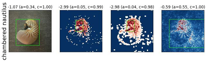
Under review as a conference paper at ICLR 2021

  GroundTruth      SMUG        SMUG base        IG           GroundTruth    SMUG        SMUG base        IG

                       (a)   Examples where SMUG outperforms other compared methods.

  GroundTruth     SMUG         SMUG base        IG          GroundTruth    SMUG        SMUG base        IG

                              (b)   Examples where SMUG performs less favorably.

Figure 1: Examples where SMUG outperforms other compared methods (top 4 rows), and where SMUG
performs less favorably (last 2 rows) based on LSC. The green box on the original image highlights the
groundtruth box; for the saliency methods it represents the bounding box with the best LSC score. Numbers on
top denote the LSC score, the fractional area of the bounding box (a), and the confidence of the classifier (c) on
the cropped region. Red and blue colors denote regions of high and low importance respectively.

SMUGbase have similar sizes even though the former produces much sparser saliency maps. This
causes both SMUG and SMUGbase to receive similar LSC scores. Thus, the LSC scores alone don’t
reveal the full picture and we need to consider the sparsity as well. This is defined as the fraction
of the pixels with non-zero attributions to the total number of pixels in the image. We find that the
average SMUGbase mask has a sparsity of 43% while the average SMUG mask has a sparsity of
just 17%. This is also evident from the examples in Fig. 1. SMUG and SMUGbase receive similar
LSC scores which suggests that the symbolic encoding successfully retains pixels relevant to the
prediction while removing about 66% pixels from SMUGbase .
G ROUND T RUTH, C ENTER B OX. Based on qualitative examples Figs. 1, we can observe that in
almost all cases the object is at the center of the image. Hence, C ENTER B OX is likely to capture
some part of the image. Further, a fair number of objects are large covering much of the image e.g.,
Fig. 1 Macaque, Collie, Robin, Dalmation. In these cases, the groundtruth bounding boxes are also
large to fully cover all pixels corresponding to the object. In contrast, SMUG saliency maps are more
compact for both large and small objects, and hence achieve a better LSC score.

5.2   D ISCUSSION : A NALYZING THE LSC METRIC AND O PT B OX

The LSC metric makes a trade-off when optimizing for both compactness and confidence. To analyze
this we look at several qualitative examples (Fig. 2) of the bounding boxes identified by the O PT B OX

                                                        7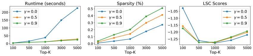
Under review as a conference paper at ICLR 2021

                            (a) OPTBOX is better than SMUG                                  (b) SMUG is better than OPTBOX

Figure 2: O PT B OX vs SMUG. 6 columns on the left correspond to the images for which O PT B OX gets a
better score than SMUG. 2 columns on the right correspond to the images for which SMUG got a better LSC
score than O PT B OX. Numbers at the top denote the LSC score, fractional area of the bounding box a and the
confidence of the classifier c on the cropped region.

      (a) catbig       (b) catsmall           (c) 2-cats         (d) 2-cats SMUG   (e) 2-cats IG     (f) 2-cats OPTBOX

Figure 3: (a) shows an image of a cat (catbig ) placed on a white background that is classified with a confidence
of 0.83. (b) shows an image of the same cat (catsmall ), scaled to a quarter of its original size, that is classified
with a confidence of 0.15. (c) By placing catbig next to catsmall we observe a significant jump in the classifier’s
confidence from 0.15 with catsmall alone to 0.84 on 2-cats. While (d) SMUG and (e) IG correctly attribute the
model confidence to catbig , (f) O PT B OX exploits the object rescaling in LSC, favoring the more compact object.

brute-force approach to optimize the LSC metric. We observe that O PT B OX often finds bounding
boxes that are very small, typically a sufficiently discriminative region or pattern in the image (e.g.,
typewriter keyboard, paddlewheel, vine snake in Fig. 2), or the full object if the object is itself small
(e.g., basketball, plunger). In all these cases we find that SMUG highlights several other aspects of
the object as well (typewriter’s tape; the dog’s eyes, nose and ears, etc.)
In particular, O PT B OX seems to exploit the fact that the LSC metric is somewhat invariant to the
size/scale of the object (because of the resizing). This can be seen from the examples in Fig. 3.
LSC favors compact regions where the model continues to have high confidence, and the O PT B OX
score (Fig. 3(f)) is very good for the box around the small cat alone. However, as evidenced from
the confidences of the model for Fig. 3 (a), (b) and (c) a good saliency map should assign greater
attribution to catbig . In this respect, both SMUG and IG capture the model’s behavior correctly.
Moreover, SMUG attributions highlight the facial and body features of catbig .

5.3    T EXT DATASET: B EER R EVIEWS

We present randomly selected qualitative examples from the test set comparing with other methods
including SIS, IG, and G ROUND T RUTH in Fig. 4 and Appendix. C. The solution of SIS consists
of multiple disjoint set of words of varying relevance. A saliency map is constructed by scoring the
words in the sets between (0,1] on the basis of relevance of the set. However, evaluation is harder.
Unlike images where the masked image can be cropped and resized as input to compute the LSC
metric, the same strategy cannot be followed on the text model. Specifically, ImageNet models are
trained with extensive data-augmentation including random crops and resizing, and the modified
image is less likely to be out-of-distribution. Whereas in the case of text, this model doesn’t employ
any form of meaningful augmentation, and the masked text is much more likely to come from a
distribution that has not been seen during training. Hence LSC is not applicable here.

                                                             8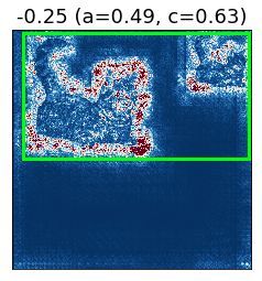
Under review as a conference paper at ICLR 2021

                         SIS                                                  SMUG                                                    SMUGbase                                                   IG
                                                                                                                                                                                                                                 1
 11.2 oz bottle split and poured into a new              11.2 oz bottle split and poured into a new              11.2 oz bottle split and poured into a new              11.2 oz bottle split and poured into a new
 belgium globe . 4.3 % abv , 4°c - 6°c , 40199           belgium globe . 4.3 % abv , 4°c - 6°c , 40199           belgium globe . 4.3 % abv , 4°c - 6°c , 40199           belgium globe . 4.3 % abv , 4°c - 6°c , 40199
 on label . a - faintly cloudy pink in color with        on label . a - faintly cloudy pink in color with        on label . a - faintly cloudy pink in color with        on label . a - faintly cloudy pink in color with
 a dense white head . frilly lace drapes                 a dense white head . frilly lace drapes                 a dense white head . frilly lace drapes                 a dense white head . frilly lace drapes                 0
 across the glass delicately . s - fresh bushels         across the glass delicately . s - fresh bushels         across the glass delicately . s - fresh bushels         across the glass delicately . s - fresh bushels
 of raspberries just rinsed gives the aroma              of raspberries just rinsed gives the aroma              of raspberries just rinsed gives the aroma              of raspberries just rinsed gives the aroma
 an inviting nose . soft wheat and lemonade              an inviting nose . soft wheat and lemonade              an inviting nose . soft wheat and lemonade              an inviting nose . soft wheat and lemonade
 pull through and 'fake-up ' the aroma . it              pull through and 'fake-up ' the aroma . it              pull through and 'fake-up ' the aroma . it              pull through and 'fake-up ' the aroma . it              -1
 almost begins smelling like a berry                     almost begins smelling like a berry                     almost begins smelling like a berry                     almost begins smelling like a berry
 weiss-sunset wheat combo . initially good               weiss-sunset wheat combo . initially good               weiss-sunset wheat combo . initially good               weiss-sunset wheat combo . initially good
 though ... t - fruity raspberry is far too              though ... t - fruity raspberry is far too              though ... t - fruity raspberry is far too              though ... t - fruity raspberry is far too
 syrupy with a lingering corn syrup finish .             syrupy with a lingering corn syrup finish .             syrupy with a lingering corn syrup finish .             syrupy with a lingering corn syrup finish .
 light wheat in the background balanced just             light wheat in the background balanced just             light wheat in the background balanced just             light wheat in the background balanced just
 a bit but it 's overly fake in it 's flavor profile .   a bit but it 's overly fake in it 's flavor profile .   a bit but it 's overly fake in it 's flavor profile .   a bit but it 's overly fake in it 's flavor profile .
 it almost seems as if lemonade is blended in            it almost seems as if lemonade is blended in            it almost seems as if lemonade is blended in            it almost seems as if lemonade is blended in
 . m - sugary sweet and slight with a highly             . m - sugary sweet and slight with a highly             . m - sugary sweet and slight with a highly             . m - sugary sweet and slight with a highly
 carbonated finish and light body . o - overly           carbonated finish and light body . o - overly           carbonated finish and light body . o - overly           carbonated finish and light body . o - overly
 sweet and fake , it 's got a good aroma                 sweet and fake , it 's got a good aroma                 sweet and fake , it 's got a good aroma                 sweet and fake , it 's got a good aroma
 initially but definitely lacking elsewhere . too        initially but definitely lacking elsewhere . too        initially but definitely lacking elsewhere . too        initially but definitely lacking elsewhere . too
 syrupy but not awful .                                  syrupy but not awful .                                  syrupy but not awful .                                  syrupy but not awful .

Figure 4: Example comparing our method (SMUG, SMUGbase ) with SIS and IG on a test sample from the
Beer Reviews dataset. Green color signifies a positive relevance, red color signifies negative relevance. The
underlined words are human annotations.

6        C ONCLUSION

We present an approach that uses SMT solvers for computing minimal input features that are relevant
for a neural network prediction. In particular, it uses attribution scores from Integrated Gradients to
find a subset of important neurons in the first layer of the network, which allows the SMT encoding
of constraints to scale to larger networks for finding minimal input masks. We evaluate our technique
to analyze models trained on image and text datasets and show that the saliency maps generated by
our approach are competitive or better than existing approaches and produce sparser masks.

R EFERENCES
David Alvarez-Melis and Tommi S Jaakkola. On the robustness of interpretability methods. arXiv
  preprint arXiv:1806.08049, 2018.

Sebastian Bach, Alexander Binder, Grégoire Montavon, Frederick Klauschen, Klaus-Robert Müller,
  and Wojciech Samek. On pixel-wise explanations for non-linear classifier decisions by layer-wise
  relevance propagation. PloS one, 10(7), 2015.

Clark Barrett and Cesare Tinelli. Satisfiability modulo theories. In Handbook of Model Checking, pp.
  305–343. Springer, 2018.

Nikolaj Bjørner, Anh-Dung Phan, and Lars Fleckenstein. νz-an optimizing smt solver. In International
  Conference on Tools and Algorithms for the Construction and Analysis of Systems, pp. 194–199.
  Springer, 2015.

Brandon Carter, Jonas Mueller, Siddhartha Jain, and David Gifford. What made you do this?
  understanding black-box decisions with sufficient input subsets. arXiv preprint arXiv:1810.03805,
  2018.

Piotr Dabkowski and Yarin Gal. Real time image saliency for black box classifiers. In Advances in
  Neural Information Processing Systems, pp. 6967–6976, 2017.

Jia Deng, Wei Dong, Richard Socher, Li-Jia Li, Kai Li, and Li Fei-Fei. Imagenet: A large-scale
   hierarchical image database. In 2009 IEEE conference on computer vision and pattern recognition,
   pp. 248–255. Ieee, 2009.

D. Gopinath, H. Converse, C. Pasareanu, and A. Taly. Property inference for deep neural networks.
  In 2019 34th IEEE/ACM International Conference on Automated Software Engineering (ASE), pp.
  797–809, 2019.

Divya Gopinath, Hayes Converse, Corina Pasareanu, and Ankur Taly. Property inference for deep
  neural networks. In 2019 34th IEEE/ACM International Conference on Automated Software
  Engineering (ASE), pp. 797–809. IEEE, 2019.

                                                                                                                 9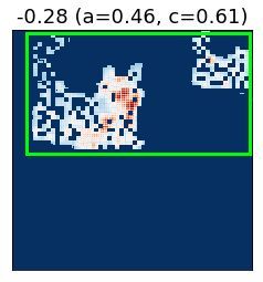
Under review as a conference paper at ICLR 2021

Sara Hooker, Dumitru Erhan, Pieter-Jan Kindermans, and Been Kim. A benchmark for interpretability
  methods in deep neural networks. In Advances in Neural Information Processing Systems, pp.
  9734–9745, 2019.
Xiaowei Huang, Marta Kwiatkowska, Sen Wang, and Min Wu. Safety verification of deep neural
  networks. In International Conference on Computer Aided Verification, pp. 3–29. Springer, 2017.
Alexey Ignatiev, Nina Narodytska, and Joao Marques-Silva. Abduction-based explanations for
  machine learning models. In Proceedings of the AAAI Conference on Artificial Intelligence,
  volume 33, pp. 1511–1519, 2019.
Andrei Kapishnikov, Tolga Bolukbasi, Fernanda Viégas, and Michael Terry. Xrai: Better attributions
  through regions. In Proceedings of the IEEE International Conference on Computer Vision, pp.
  4948–4957, 2019.
Guy Katz, Clark Barrett, David Dill, Kyle Julian, and Mykel Kochenderfer. Reluplex: An efficient
  smt solver for verifying deep neural networks, 2017.
Yann LeCun, Corinna Cortes, and CJ Burges. Mnist handwritten digit database. 2010.
Jan Macdonald, Stephan Wäldchen, Sascha Hauch, and Gitta Kutyniok. A rate-distortion framework
  for explaining neural network decisions. arXiv preprint arXiv:1905.11092, 2019.
Julian McAuley, Jure Leskovec, and Dan Jurafsky. Learning attitudes and attributes from multi-aspect
  reviews. In 2012 IEEE 12th International Conference on Data Mining, pp. 1020–1025. IEEE,
  2012.
Ramprasaath R Selvaraju, Abhishek Das, Ramakrishna Vedantam, Michael Cogswell, Devi Parikh,
  and Dhruv Batra. Grad-cam: Why did you say that? arXiv preprint arXiv:1611.07450, 2016.
Ramprasaath R Selvaraju, Michael Cogswell, Abhishek Das, Ramakrishna Vedantam, Devi Parikh,
  and Dhruv Batra. Grad-cam: Visual explanations from deep networks via gradient-based local-
  ization. In Proceedings of the IEEE international conference on computer vision, pp. 618–626,
  2017.
Dylan Slack, Sophie Hilgard, Emily Jia, Sameer Singh, and Himabindu Lakkaraju. Fooling lime
  and shap: Adversarial attacks on post hoc explanation methods. In Proceedings of the AAAI/ACM
 Conference on AI, Ethics, and Society, pp. 180–186, 2020.
Daniel Smilkov, Nikhil Thorat, Been Kim, Fernanda Viégas, and Martin Wattenberg. Smoothgrad:
  removing noise by adding noise. arXiv preprint arXiv:1706.03825, 2017.
Saurabh Srivastava, Sumit Gulwani, and Jeffrey S Foster. Vs 3: Smt solvers for program verification.
  In International Conference on Computer Aided Verification, pp. 702–708. Springer, 2009.
Pascal Sturmfels, Scott Lundberg, and Su-In Lee. Visualizing the impact of feature attribution
  baselines. Distill, 2020. doi: 10.23915/distill.00022. https://distill.pub/2020/attribution-baselines.
Mukund Sundararajan, Ankur Taly, and Qiqi Yan. Axiomatic attribution for deep networks. In Doina
 Precup and Yee Whye Teh (eds.), Proceedings of the 34th International Conference on Machine
 Learning, ICML 2017, Sydney, NSW, Australia, 6-11 August 2017, volume 70 of Proceedings
 of Machine Learning Research, pp. 3319–3328. PMLR, 2017. URL http://proceedings.
 mlr.press/v70/sundararajan17a.html.
Christian Szegedy, Wei Liu, Yangqing Jia, Pierre Sermanet, Scott Reed, Dragomir Anguelov, Du-
  mitru Erhan, Vincent Vanhoucke, and Andrew Rabinovich. Going deeper with convolutions. In
  Proceedings of the IEEE conference on computer vision and pattern recognition, pp. 1–9, 2015.
Shawn Xu, Subhashini Venugopalan, and Mukund Sundararajan. Attribution in scale and space.
  arXiv preprint arXiv:2004.03383, 2020.
Xin Zhang, Armando Solar-Lezama, and Rishabh Singh. Interpreting neural network judgments via
  minimal, stable, and symbolic corrections. In Advances in Neural Information Processing Systems,
  pp. 4874–4885, 2018.

                                                  10
Under review as a conference paper at ICLR 2021
A PPENDIX
Here, we present additional quantitative and qualitative examples supporting the results in Sec. 5. In
particular Sec. A shows qualitative examples on MNIST, Sec. B presents quantitative and qualitative
comparisons with regard to the choice of key parameters of our proposed SMUG explanation
technique. Sec. C presents additional qualitative examples comparing the output of SMUG with
other methods on text samples from the Beer Reviews dataset. Sec. D presents several more qualitative
examples from ImageNet comparing the saliency masks produced by SMUG with those produced by
other methods. In Sec. D.1 we also discuss an example where an explanation technique can be used
to identify potential biases of the trained model. Finally, Sec. E presents some examples of concrete
constraints that the solver optimizes.
A MNIST
In this section, we present some more details about our experiments with MNIST using the full SMT
encoding from Eq. 1 in Sec 3.1.
SMT solvers can be used to encode the semantics of a neural network (Katz et al., 2017). In particular,
given a fully connected neural network with n hidden layers, weights W = {W1 , W2 . . . , Wn }, biases
B = {b1 , b2 . . . , bn }, activation function φ, and final layer softmax σ, we can use the SMT theory
of nonlinear real arithmetic to obtain a symbolic encoding of the network. Let X ∈ Rm×n denote
an input image with m × n pixels, M ∈ {0, 1}m×n an unknown binary mask, Li the output (i.e.,
activations) of the ith layer (L0 = X is the input) and α(pj ) the output of j th logit in the final layer:
Li ≡ φ(Wi Li−1 + bi ) α(pj , W, B, X) ≡ σj (Wn Ln−1 + bn )
Given this symbolic encoding, we can encode the minimal input mask generation problem as:
∃M : minimize(Σij Mij ) ∧ α(plabel , W, B, M X) > α(pl , W, B, M X) ∀l 6= label (6)
where plabel and pl refer to the logits corresponding to the true label and the other labels respectively.
The number of constraints grow with increasing network size and SMT decision procedure for Non-
linear Real Arithmetic is doubly exponential. Even for piecewise ReLU networks, SMT decision
procedures for Linear Real Arithmetic combine simplex-based methods (exponential complexity)
with other decision procedures such as Boolean logic (NP-complete complexity), which causes the
solving times to grow dramatically with network size. When we apply this encoding even for a small
feed-forward network on MNIST dataset, the SMT solver does not scale well (Section 4). This
motivates our proposed approach for using gradient information to simplify the SMT constraints.
Table 2 shows the SMT solver runtimes and whether the constraints were solved (S AT). We observe
that with a timeout of 60 minutes, the SMT solver could solve the full constraints for only 34 of
the 100 images. Another interesting point to observe is that the solver could not solve any of the
instances for digits 0 and 3. We also show some of the minimal masks generated by the SMT solver
for few MNIST images in Figure 5.
Table 2: Solver Runtime and SAT instances. We report the average solver runtime and instances
solved per digit with a timeout set at 60 mins.
Digit 0 1 2 3 4 5 6 7 8 9 ALL
Runtime (mins) N.A. 31.19 45.26 N.A. 33.09 35.68 42.80 53.11 36.05 19.62 35.59
SAT Instances 0/8 8/14 4/8 0/11 8/14 4/7 4/10 2/15 1/2 3/11 34/100
11Under review as a conference paper at ICLR 2021
Image Mask Image Mask Image Mask Image Mask
Figure 5: MNIST images and the corresponding masks corresponding to Sec. 3.1.
B H YPERPARAMETER C HOICES
In our proposed approach, the choice of top-k, and γ (Eqns. 3, 4, 5) have an effect on the final quality
of the explanations, and the time it takes for the solver to identify the mask. This section presents
quantitative and qualitative comparisons for different choices of top-k and γ.
B.1 Q UANTITATIVE COMPARISON FOR DIFFERENT CHOICES OF TOP -k AND γ
Fig. 6 presents quantitative comparisons for different choices of top-k and γ.
Figure 6: Hyperparameter Comparision
top-k We analyze images with top-k ∈ {500, 1000, 3000, 5000}. Increasing the k value increases the
receptive field and the discovered input masks also grow in size with increasing values of k. Figure 6
shows how the solver runtime and the mask size vary with k. As expected, larger k values results in
larger number of constraints and therefore larger solving times as well as larger mask sizes.
Gamma We analyze the effect of γ ∈ {0.0, 0.5, 0.9}, also shown in in Fig. 6. We observe that by
decreasing gamma values, the masks become sparser. The key reason behind this is that with smaller
gamma values, the SMTsolver is less constrained to maintain the original neural activations for the
selected neurons, and hence can ignore additional input pixels that do not have a large effect. It is
also noteworthy to notice that the solver run-time increases with decreasing value of γ.
12Under review as a conference paper at ICLR 2021
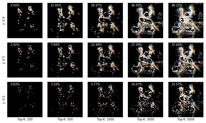
B.2 T OP - K VS γ ON I MAGE N ET - Q UALITATIVE EXAMPLES
Fig. 7 presents qualitative examples of the saliency maps on Imagenet examples for different choices
of top-k and γ.
Figure 7: Qualitative examples of the masks generated by SMUG on examples from Imagenet for
different choices of top-k (columns) and γ (rows). γ = 0 is the most minimal mask. Even at low
values of top-k and γ SMUG highlights pixels relevant for the object class.
13Under review as a conference paper at ICLR 2021
C Q UALITATIVE TEXT EXAMPLES
Fig. 8 presents additional examples comparing the output of SMUG with SIS, SMUGbase , and IG on
the Beer Reviews dataset.
SIS SMUG SMUGbase IG
1
very dark beer . pours a nice finger and a very dark beer . pours a nice finger and a very dark beer . pours a nice finger and a very dark beer . pours a nice finger and a
half of creamy foam and stays throughout half of creamy foam and stays throughout half of creamy foam and stays throughout half of creamy foam and stays throughout
the beer . smells of coffee and roasted malt the beer . smells of coffee and roasted malt the beer . smells of coffee and roasted malt the beer . smells of coffee and roasted malt
. has a major coffee-like taste with hints of . has a major coffee-like taste with hints of . has a major coffee-like taste with hints of . has a major coffee-like taste with hints of 0
chocolate . if you like black coffee , you will chocolate . if you like black coffee , you will chocolate . if you like black coffee , you will chocolate . if you like black coffee , you will
love this porter . creamy smooth mouthfeel love this porter . creamy smooth mouthfeel love this porter . creamy smooth mouthfeel love this porter . creamy smooth mouthfeel
and definitely gets smoother on the palate and definitely gets smoother on the palate and definitely gets smoother on the palate and definitely gets smoother on the palate
once it warms . it 's an ok porter but i feel once it warms . it 's an ok porter but i feel once it warms . it 's an ok porter but i feel once it warms . it 's an ok porter but i feel -1
there are much better one 's out there . there are much better one 's out there . there are much better one 's out there . there are much better one 's out there .
SIS SMUG SMUGbase IG
1
poured into a snifter . produces a small poured into a snifter . produces a small poured into a snifter . produces a small poured into a snifter . produces a small
coffee head that reduces quickly . black as coffee head that reduces quickly . black as coffee head that reduces quickly . black as coffee head that reduces quickly . black as
night . pretty typical imp . roasted malts hit night . pretty typical imp . roasted malts hit night . pretty typical imp . roasted malts hit night . pretty typical imp . roasted malts hit
on the nose . a little sweet chocolate follows on the nose . a little sweet chocolate follows on the nose . a little sweet chocolate follows on the nose . a little sweet chocolate follows 0
. big roasty character on the taste . in . big roasty character on the taste . in . big roasty character on the taste . in . big roasty character on the taste . in
between i 'm getting plenty of dark between i 'm getting plenty of dark between i 'm getting plenty of dark between i 'm getting plenty of dark
chocolate and some bitter espresso . it chocolate and some bitter espresso . it chocolate and some bitter espresso . it chocolate and some bitter espresso . it
finishes with hop bitterness . nice smooth finishes with hop bitterness . nice smooth finishes with hop bitterness . nice smooth finishes with hop bitterness . nice smooth -1
mouthfeel with perfect carbonation for the mouthfeel with perfect carbonation for the mouthfeel with perfect carbonation for the mouthfeel with perfect carbonation for the
style . overall a nice stout i would love to style . overall a nice stout i would love to style . overall a nice stout i would love to style . overall a nice stout i would love to
have again , maybe with some age on it . have again , maybe with some age on it . have again , maybe with some age on it . have again , maybe with some age on it .
SIS SMUG SMUGbase IG
1
a very underrated ipa pours a a very underrated ipa pours a a very underrated ipa pours a a very underrated ipa pours a
coppery/burnt orange color with a big head coppery/burnt orange color with a big head coppery/burnt orange color with a big head coppery/burnt orange color with a big head
that lasts quite some time . taste is hoppy , that lasts quite some time . taste is hoppy , that lasts quite some time . taste is hoppy , that lasts quite some time . taste is hoppy ,
with loads of pine-y bitterness , but also with loads of pine-y bitterness , but also with loads of pine-y bitterness , but also with loads of pine-y bitterness , but also 0
citrus flavors including grapefruit and ... is citrus flavors including grapefruit and ... is citrus flavors including grapefruit and ... is citrus flavors including grapefruit and ... is
that a hint of tropical flavor ? maybe some that a hint of tropical flavor ? maybe some that a hint of tropical flavor ? maybe some that a hint of tropical flavor ? maybe some
pineapple . you see some nice malt/hop pineapple . you see some nice malt/hop pineapple . you see some nice malt/hop pineapple . you see some nice malt/hop
balance in quite a few of the better dipas , balance in quite a few of the better dipas , balance in quite a few of the better dipas , balance in quite a few of the better dipas , -1
but this is one of the few ipas that 's both but this is one of the few ipas that 's both but this is one of the few ipas that 's both but this is one of the few ipas that 's both
quite hoppy and well balanced superb quite hoppy and well balanced superb quite hoppy and well balanced superb quite hoppy and well balanced superb
mouthfeel and drinkability . ballast point mouthfeel and drinkability . ballast point mouthfeel and drinkability . ballast point mouthfeel and drinkability . ballast point
continues to rise in my estimation with continues to rise in my estimation with continues to rise in my estimation with continues to rise in my estimation with
every offering i consume . every offering i consume . every offering i consume . every offering i consume .
SIS SMUG SMUGbase IG
1
poured from a 24oz bottle into a large poured from a 24oz bottle into a large poured from a 24oz bottle into a large poured from a 24oz bottle into a large
sniffter appearance : this pours a deep sniffter appearance : this pours a deep sniffter appearance : this pours a deep sniffter appearance : this pours a deep
bronze amber in color . this beer has some bronze amber in color . this beer has some bronze amber in color . this beer has some bronze amber in color . this beer has some
of the best head formation and retention of the best head formation and retention of the best head formation and retention of the best head formation and retention 0
that i have ever seen along with lots and lots that i have ever seen along with lots and lots that i have ever seen along with lots and lots that i have ever seen along with lots and lots
of sticky lacing smell : tons of piney resinous of sticky lacing smell : tons of piney resinous of sticky lacing smell : tons of piney resinous of sticky lacing smell : tons of piney resinous
evergreen aroms abound in this ale . cant evergreen aroms abound in this ale . cant evergreen aroms abound in this ale . cant evergreen aroms abound in this ale . cant
get enough of this beer its the best smelling get enough of this beer its the best smelling get enough of this beer its the best smelling get enough of this beer its the best smelling -1
harvest ale i 've ever had the pleasure of harvest ale i 've ever had the pleasure of harvest ale i 've ever had the pleasure of harvest ale i 've ever had the pleasure of
enjoying taste : huge flavor profile with lots enjoying taste : huge flavor profile with lots enjoying taste : huge flavor profile with lots enjoying taste : huge flavor profile with lots
of bitterness and only a little malt sweetness of bitterness and only a little malt sweetness of bitterness and only a little malt sweetness of bitterness and only a little malt sweetness
. as this beer warms up the bitterness really . as this beer warms up the bitterness really . as this beer warms up the bitterness really . as this beer warms up the bitterness really
dominates the flavor . i 'm tasting lot of dominates the flavor . i 'm tasting lot of dominates the flavor . i 'm tasting lot of dominates the flavor . i 'm tasting lot of
subtle orange aromas mouthfeel : full body subtle orange aromas mouthfeel : full body subtle orange aromas mouthfeel : full body subtle orange aromas mouthfeel : full body
beer with alot of carbonation overall : i love beer with alot of carbonation overall : i love beer with alot of carbonation overall : i love beer with alot of carbonation overall : i love
this beer in my opinion its serria nevada 's this beer in my opinion its serria nevada 's this beer in my opinion its serria nevada 's this beer in my opinion its serria nevada 's
best beer overall . the price is unbeatable i best beer overall . the price is unbeatable i best beer overall . the price is unbeatable i best beer overall . the price is unbeatable i
bought my bombed for $ 3.99 . so much bought my bombed for $ 3.99 . so much bought my bombed for $ 3.99 . so much bought my bombed for $ 3.99 . so much
flavor and biting bitterness this harvest ale flavor and biting bitterness this harvest ale flavor and biting bitterness this harvest ale flavor and biting bitterness this harvest ale
has no equal . has no equal . has no equal . has no equal .
SIS SMUG SMUGbase IG
1
poured from a 12oz bottle into a delirium poured from a 12oz bottle into a delirium poured from a 12oz bottle into a delirium poured from a 12oz bottle into a delirium
tremens glass . this is so hard to find in tremens glass . this is so hard to find in tremens glass . this is so hard to find in tremens glass . this is so hard to find in
columbus for some reason , but i was able columbus for some reason , but i was able columbus for some reason , but i was able columbus for some reason , but i was able
to get it in toledo ... murky yellow to get it in toledo ... murky yellow to get it in toledo ... murky yellow to get it in toledo ... murky yellow 0
appearance with a very thin white head . the appearance with a very thin white head . the appearance with a very thin white head . the appearance with a very thin white head . the
aroma is bready and a little sour . the flavor aroma is bready and a little sour . the flavor aroma is bready and a little sour . the flavor aroma is bready and a little sour . the flavor
is really complex , with at least the following is really complex , with at least the following is really complex , with at least the following is really complex , with at least the following
tastes : wheat , spicy hops , bread , bananas tastes : wheat , spicy hops , bread , bananas tastes : wheat , spicy hops , bread , bananas tastes : wheat , spicy hops , bread , bananas -1
, and a toasty after-taste . it was really , and a toasty after-taste . it was really , and a toasty after-taste . it was really , and a toasty after-taste . it was really
outstanding . i 'd recommend this to anyone outstanding . i 'd recommend this to anyone outstanding . i 'd recommend this to anyone outstanding . i 'd recommend this to anyone
, go out and try it . i think it 's the best so far , go out and try it . i think it 's the best so far , go out and try it . i think it 's the best so far , go out and try it . i think it 's the best so far
from this brewery . from this brewery . from this brewery . from this brewery .
Figure 8: Examples comparing our method (SMUG, SMUGbase ) with SIS and IG on test samples
from the Beer Reviews dataset. Green color signifies a positive relevance, red color signifies negative
relevance. The underlined words are human annotations.
D A DDITIONAL QUALITATIVE IMAGE EXAMPLES : SMUG
Fig. 9 presents boolean masks and the saliency maps produced by SMUG on several ImageNet
examples. Fig. 10 and 11 present additional examples comparing the saliency masks and bounding
box (for LSC) produced by SMUG, SMUGbase , and IG.
14You can also read