INTERPRETATIONS ARE USEFUL: PENALIZING EXPLA-NATIONS TO ALIGN NEURAL NETWORKS WITH PRIOR KNOWLEDGE
←
→
Page content transcription
If your browser does not render page correctly, please read the page content below
Under review as a conference paper at ICLR 2020

I NTERPRETATIONSARE USEFUL : PENALIZING EXPLA -
NATIONS TO ALIGN NEURAL NETWORKS WITH PRIOR
KNOWLEDGE

 Anonymous authors
 Paper under double-blind review

                                            A BSTRACT

         For an explanation of a deep learning model to be effective, it must provide both
         insight into a model and suggest a corresponding action in order to achieve some
         objective. Too often, the litany of proposed explainable deep learning methods
         stop at the first step, providing practitioners with insight into a model, but no
         way to act on it. In this paper, we propose contextual decomposition explanation
         penalization (CDEP), a method which enables practitioners to leverage existing
         explanation methods in order to increase the predictive accuracy of deep learn-
         ing models. In particular, when shown that a model has incorrectly assigned im-
         portance to some features, CDEP enables practitioners to correct these errors by
         directly regularizing the provided explanations. Using explanations provided by
         contextual decomposition (CD) (Murdoch et al., 2018), we demonstrate the ability
         of our method to increase performance on an array of toy and real datasets.

1   I NTRODUCTION

In recent years, neural networks have demonstrated strong predictive performance across a wide
variety of settings. However, in order to achieve that accuracy, they sometimes latch onto spurious
correlations, leading to undesirable behavior as a result of dataset bias (Winkler et al., 2019), racial
and ethnic stereotypes (Garg et al., 2018), or simply overfitting. While recent work into explaining
neural network predictions (Murdoch et al., 2019; Doshi-Velez & Kim, 2017) has demonstrated an
ability to uncover the relationships learned by a model, it is still unclear how to actually alter the
model in order to remove incorrect, or undesirable, relationships.
We introduce contextual decomposition explanation penalization (CDEP), a method which lever-
ages existing explanation techniques for neural networks in order to prevent a model from learning
unwanted relationships and ultimately improve predictive accuracy.
Given particular importance scores, CDEP works by allowing the user to directly penalize impor-
tances of certain features, or interactions. This forces the neural network to not only produce the
correct prediction, but also the correct explanation for that prediction. While we focus on contextual
decomposition (CD) (Murdoch et al., 2018; Singh et al., 2018), which allows the penalization of
both feature importances and interactions, CDEP can be readily adapted for existing interpretation
techniques, as long as they are differentiable. Moreover, CDEP is a general technique, which can
be applied to arbitrary neural network architectures, and is orders of magnitude faster and more
memory efficient than recent gradient-based methods, allowing its use on meaningful datasets.
In order to demonstrate the effectiveness of CDEP, we conducted experiments across a wide variety
of tasks. In the prediction of skin cancer from images, CDEP improves the prediction of a classifier
by teaching it to ignore spurious confounding variables present in the training data. In a colored
MNIST task, CDEP allows the network to focus on a digit’s shape rather than its color (with no
extra human annotation needed). Finally, a toy example using text classification shows how the
penalization can help a network avoid a bias towards particular words, such as those involving
gender.

                                                   1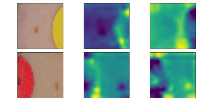
Under review as a conference paper at ICLR 2020

                                              Prediction                   Label

                                              Explanation                Desired
                                                                        Explanation

Figure 1: CDEP allows a practitioner to penalize both a model’s prediction and the corresponding
explanation.

2   BACKGROUND
Explanation methods Many methods have been developed to help explain the learned relation-
ships contained in a DNN. For local, or prediction-level, explanation, most prior work has focused
on assigning importance to individual features, such as pixels in an image or words in a document.
There are several methods that give feature-level importance for different architectures. They can
be categorized as gradient-based (Springenberg et al., 2014; Sundararajan et al., 2017; Selvaraju
et al., 2016; Baehrens et al., 2010; Rieger & Hansen, 2019), decomposition-based (Murdoch &
Szlam, 2017; Shrikumar et al., 2016; Bach et al., 2015) and others (Dabkowski & Gal, 2017; Fong
& Vedaldi, 2017; Ribeiro et al., 2016; Zintgraf et al., 2017), with many similarities among the meth-
ods (Ancona et al., 2018; Lundberg & Lee, 2017). However, many of these methods have thus far
been poorly evaluated (Adebayo et al., 2018; Nie et al., 2018), casting doubt on their usefulness. An-
other line of work, which we build upon, has focused on uncovering interactions between features,
in addition to feature importances, (Murdoch et al., 2018), and using those interactions to create a
hierarchy of features displaying the model’s prediction process (Singh et al., 2018).

Uses of explanation methods While much work has been put into developing methods for ex-
plaining DNNs, relatively little work has explored the potential to use these explanations to help
build a better model. Some recent work proposes forcing models to attend to regions of the input
which are known to be important (Burns et al., 2018; Mitsuhara et al., 2019), although it is important
to note that attention is often not the same as explanation (Jain & Wallace, 2019). An alternative
line of work proposes penalizing the gradients of a neural network to match human-provided binary
annotations and shows the possibility to improve performance (Ross et al., 2017) and adversarial
robustness (Ross & Doshi-Velez, 2018). Two recent papers extend these ideas by penalizing attri-
butions for natural language models (Liu & Avci, 2019) and penalizing a modified gradient-based
score to produce smooth attributions (Erion et al., 2019). Predating deep learning, (Zaidan et al.,
2007) consider the use of “annotator rationales” in sentiment analysis to train support vector ma-
chines. This work on annotator rationales was recently extended to show improved explanations
(not accuracy) in CNNs (Strout et al., 2019).

Other ways to constrain DNNs While we focus on the use of explanations to constrain the rela-
tionships learned by neural networks, other approaches for constraining neural networks have also
been proposed. A computationally intensive alternative is to augment the dataset in order to prevent
the model from learning undesirable relationships, through domain knowledge (Bolukbasi et al.,
2016), projecting out superficial statistics (Wang et al., 2019) or dramatically altering training im-
ages (Geirhos et al., 2018). However, these processes are often not feasible, either due to their
computational cost or the difficulty of constructing such an augmented data set. Adversarial training
has also been explored (Zhang & Zhu, 2019). These techniques are generally limited, as they are
often tied to particular datasets, and do not provide a clear link between learning about a model’s
learned relationships through explanations, and subsequently correcting them.

3   M ETHODS
We now introduce CDEP, which penalizes the explanations of a neural network in order to align
with prior knowledge about why a model should make a prediction. To do so, for each data point

                                                  2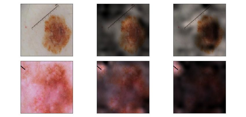
Under review as a conference paper at ICLR 2020

it penalizes the CD scores of features, or groups of features, which a user does not want the model
to learn to be important. While we focus on CD scores, which allow the penalization of interac-
tions between features in addition to features themselves, this approach readily generalizes to other
interpretation techniques, so long as they are differentiable.

3.1   AUGMENTING THE LOSS FUNCTION

Given a particular classification task, we want to teach a model to not only produce the correct
prediction, but also to arrive at the prediction for the correct reasons. That is, we want the model
to be right for the right reasons, where the right reasons are provided by the user and are dataset-
dependent.
To accomplish this, CDEP modifies the objective function used to train a neural network, as dis-
played in Eq 1. In addition to the standard prediction loss L, which teaches the model to produce the
correct predictions, CDEP adds an explanation error Lexpl , which teaches the model to produce the
correct explanations for its predictions. In place of the prediction and labels fθ (X), y, used in the
prediction error L, the explanation error Lexpl uses the explanations produced by an interpretation
method explθ (X), along with targets provided by the user explX . As is common with penalization,
the two losses are weighted by a hyperparameter λ ∈ R:

                       θ̂ = argmin L (fθ (X), y) +λ Lexpl (explθ (X), explX )                      (1)
                               θ   |     {z    }    |          {z          }
                                     Prediction error       Explanation error

The precise meanings of explX depend on the context. For example, in the skin cancer image
classification task described in Section 4, many of the benign skin images contain band-aids, but
none of the malignant images. To force the model to ignore the band-aids in making their prediction,
in each image explθ (X) denotes the importance score of the band-aid and explX would be zero.
These and more examples are further explored in Section 4.

3.2   C ONTEXTUAL DECOMPOSITION (CD)

In this work, we use the CD score as the explanation function. In contrast to other interpretation
methods, which focus on feature importances, CD also captures interactions between features. CD
was originally designed for LSTMs (Murdoch et al., 2018) and subsequently extended to convolu-
tional neural networks and arbitrary DNNs (Singh et al., 2018). For a given DNN f (x), one can
represent its output as a SoftMax operation applied to logits g(x). These logits, in turn, are the
composition of L layers gi , such as convolutional operations or ReLU non-linearities.
                  f (x) = SoftMax(g(x)) = SoftMax(gL (gL−1 (...(g2 (g1 (x))))))                    (2)

Given a group of features {xj }j∈S , the CD algorithm, g CD (x), decomposes the logits g(x) into
a sum of two terms, β(x) and γ(x). β(x) is the importance score of the feature group {xj }j∈S ,
and γ(x) captures contributions to g(x) not included in β(x). The decomposition is computed by
iteratively applying decompositions giCD (x) for each of the layers gi (x).

                      g CD (x) = gL
                                  CD CD
                                    (gL−1 (...(g2CD (g1CD (x)))))) = (β(x), γ(x))                  (3)
                 β(x) + γ(x) = g(x)                                                                (4)

3.3   CDEP OBJECTIVE FUNCTION

We now substitute the above CD scores into the generic equation in Eq 1 to arrive at the method used
in this paper. While we use CD for the explanation method explθ (X), other explanation methods
could be readily substituted at this stage. In order to convert CD scores to probabilities, we apply a
SoftMax operation to g CD (x), allowing for easier comparison with the user-provided labels explX .
We collect from the user, for each input xi , a collection of feature groups xi,S , xi ∈ Rd , S ⊆
{1, ..., d}, along with explanation target values explxi,S , and use the k · k1 loss for Lexpl .

                                                        3
Under review as a conference paper at ICLR 2020

                               XX                                         XX
                 θ̂ = argmin                 − yi,c log fθ (xi )c + λ             ||β(xi,S ) − explxi,S ||1   (5)
                         θ         i   c                                  i   S
                               |                   {z             }   |                 {z               }
                                           Classification error                   Explanation error

In the above, i indexes each individual example in the dataset, S indexes a subset of the features for
which we penalize their explanations, and c sums over each class. Updating the model parameters
in accordance with this formulation ensures that the model not only predicts the right output but also
does so for the right (aligned with prior knowledge) reasons.

3.4       C OMPUTATIONAL CONSIDERATIONS

A similar idea to Eq 1 has been proposed in previous/concurrent work, where the choice of explana-
tion method uses a gradient-based attribution method (Ross et al., 2017; Erion et al., 2019). How-
ever, using such methods leads to three main complications which are solved by our approach. The
first complication is the optimization process. When optimizing over attributions from a gradient-
based attribution method via gradient descent, the optimizer requires the gradient of the gradient,
thus requiring that all network components be twice differentiable. This process is computationally
expensive and indeed optimizing it exactly involves optimizing over a differential equation. In con-
trast, CD attributions are calculated along with the forward pass of the network, and as a result can be
optimized plainly with back-propagation using the standard single forward-pass and backward-pass
per batch.
A second complication solved by the use of CD in Eq 5 is the ability to quickly finetune a pre-trained
network. In many applications, particularly in transfer learning, it is common to finetune only the
last few layers of a pre-trained neural network. Using CD, one can freeze early layers of the network
and then finetune the last few layers of the network quickly as the activations and gradients of the
frozen layers are not necessary.
Third, penalizing gradient-based methods incurs a very large memory usage. Using gradient-based
methods, training requires the storage of activations and gradients for all layers of the network as
well as the gradient of input (which can be omitted in normal training). Even for the simplest version,
based on saliency, this more than doubles the required memory for a given batch and network size.
More advanced methods proved to be completely infeasible to apply to a real-life dataset used, since
the memory requirements were too high. By contrast, penalizing CD only requires a small constant
amount of memory more than standard training.

4       R ESULTS
The results here demonstrate the efficacy of CDEP on a variety of datasets using diverse explanation
types. Sec 4.1 shows results on ignoring spurious patches in the ISIC skin cancer dataset (Codella
et al., 2019), Sec 4.2 details experiments on converting a DNN’s preference for color to a preference
for shape on a variant of the MNIST dataset (LeCun, 1998), and Sec 4.3 shows experiments on text
data from the Stanford Sentiment Treebank (SST) (Socher et al., 2013).1

4.1       I GNORING SPURIOUS SIGNALS IN SKIN CANCER DIAGNOSIS

In recent years, deep learning has achieved impressive results in diagnosing skin cancer, with predic-
tive accuracy sometimes comparable to human doctors (Esteva et al., 2017). However, the datasets
used to train these models often include spurious features which make it possible to attain high test
accuracy without learning the underlying phenomena (Winkler et al., 2019). In particular, a pop-
ular dataset from ISIC (International Skin Imaging Collaboration) has colorful patches present in
approximately 50% of the non-cancerous images but not in the cancerous images (Codella et al.,
2019). An unpenalized DNN learns to look for these patches as an indicator for predicting that an
image is benign. We use CDEP to remedy this problem by penalizing the DNN placing importance
on the patches during training.
    1
        All models were trained in PyTorch.

                                                                  4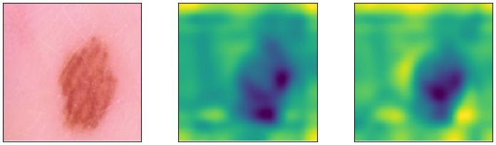
Under review as a conference paper at ICLR 2020

                                              Benign

                                                              half of data polluted with patches
                                             Malignant

Figure 2: Example images from the ISIC dataset. Half of the benign lesion images include a patch
in the image.

The task in this section is to classify whether an image of a skin lesion contains (1) benign melanoma
or (2) malignant melanoma. The ISIC dataset consists of 21,654 images (19,372 benign), each diag-
nosed by histopathology or a consensus of experts. For classification, we use a VGG16 architecture
(Simonyan & Zisserman, 2014) pre-trained on the ImageNet Classification task 2 and freeze the
weights of early layers so that only the fully connected layers are trained. In order to use CDEP, the
spurious patches are identified via a s imple image segmentation algorithm using a color threshold
(see Sec S4).
Table 1 shows results comparing the performance of a model trained with and without CDEP. We
report results on two variants of the test set. The first, which we refer to as “no patches” only
contains images of the test set that do not include patches. The second also includes images with
those patches. Training with CDEP improves the AUC and F1-score for both test sets.

Table 1: Results from training a DNN on ISIC to recognize skin cancer (averaged over three runs).
Results shown for the entire test set and for only the images the test set that do not include patches
(“no patches”). The network trained with CDEP generalizes better, getting higher AUC and F1 on
both. Std below 0.006 for all AUC and below 0.012 for all F1.
                                AUC (no patches) F1 (no patches) AUC (all) F1 (all)

       Vanilla (excluded data)                0.86               0.59                   0.92       0.59
       Vanilla                                0.85               0.56                   0.92       0.56
       With RRR                               0.66               0.39                   0.82       0.39
       With CDEP                              0.88               0.61                   0.93       0.61

In the first row of Table 1, the model is trained using only the data without the spurious patches,
and the second row shows the model trained on the full dataset. The network trained using CDEP
achieves the best AUC, surpassing both unpenalized versions. Applying our method increases the
ROC AUC as well as the best F1 score. We also compared our method against the method introduced
in 2017 by Ross et al. (RRR). For this, we restricted the batch size to 16 (and consequently use a
learning rate of 10−5 ) due to memory constraints. Using RRR did not improve on the base AUC,
implying that penalizing gradients is not helpful in penalizing higher-order features.3

Visualizing explanations Fig. 3 visualize GradCAM heatmaps (Ozbulak, 2019; Selvaraju et al.,
2017) for an unpenalized DNN and a DNN trained with CDEP to ignore spurious patches. As
expected, after penalizing with CDEP, the DNN attributes less importance to the spurious patches,
regardless of their position in the image. More examples, also for cancerous images, are shown in
Sec S5.
   2
    Pre-trained model retrieved from torchvision.
   3
    We were not able to compare against the method recently proposed in Erion et al. (2019) due to the
prohibitively slow training and large memory requirements.

                                                  5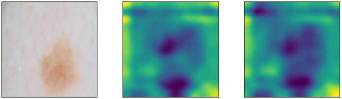
Under review as a conference paper at ICLR 2020

                         Image                  Vanilla                  CDEP

                                                                                        CDEP eliminates attention
                                                                                        on spurious patch

Figure 3: Visualizing heatmaps for correctly predicted exampes from the ISIC skincancer test set.
Lighter regions in the heatmap are attributed more importance. The DNN trained with CDEP cor-
rectly captures that the patch is not relevant for classification.

4.2      C OMBATING INDUCTIVE BIAS ON VARIANTS OF THE MNIST DATASET

In this section, we investigate whether we can alter which features a DNN uses to perform digit
classification, using variants of the MNIST dataset (LeCun, 1998) and a standard CNN architecture
for this dataset retrieved from PyTorch 4 .

4.2.1      C OLOR MNIST
Similar to a previous study (Li & Vasconcelos, 2019), we transform the MNIST dataset to include
three color channels and assign each class a distinct color, as shown in Fig. 4. An unpenalized DNN
trained on this biased data will completely misclassify a test set with inverted colors, dropping to
0% accuracy (see Section 4.2.1), suggesting that it learns to classify using the colors of the digits
rather than their shape.
Here, we want to see if we can alter the DNN to focus on the shape of the digits rather than their
color. Interestingly, this can be enforced by minimizing the contribution of pixels in isolation while
maximizing the importance of groups of pixels (which can represent shapes). To do this, we add
penalize the CD contribution of sampled single pixel values, following Eq 5. By minimizing the
contribution of single pixels we effectively encourage the network to focus more on groups of pixels,
which can represent shape.

Figure 4: ColorMNIST: the test set shapes remain the same as the training set, but the colors are
inverted. A vanilla network trained on this training set will get 0% accuracy on the test set.

Section 4.2.1 shows that CDEP can partially change the network’s focus on solely color to also
focus on digit shape. We compare CDEP to two previously introduced explanation penalization
techniques: penalization of the squared gradients (RRR) (Ross et al., 2017) and Expected Gradients
(EG) (Erion et al., 2019). For EG we penalize variance between attributions of the RGB channels
   4
       Model and training code from https://github.com/pytorch/examples/blob/master/mnist/main.py.

                                                      6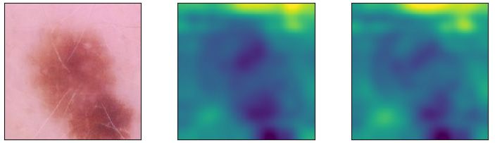
Under review as a conference paper at ICLR 2020

(as recommended by the authors of EG in personal correspondence). None of the baselines are able
to improve the test accuracy of the model on this task above the random baseline, while CDEP is
able to significantly improve this accuracy to 31.0%. We show the increase of predictive accuracy
with increasing penalization in Fig. S5.

Table 2: Results on ColorMNIST (test accuracy). All values averaged over thirty runs. CDEP is the
only method that captures and removes color bias.
                          Unpenalized       Baseline       CDEP           RRR         Expected Gradients
       Test Accuracy       0.2 ± 0.2          9.8        31.0 ± 2.3     0.2 ± 0.1        10.0 ± 0.1

4.2.2      D ECOY MNIST
For further comparison with previous work, we evaluate CDEP on an existing task: DecoyMNIST
(Erion et al., 2019). DecoyMNIST adds a class-indicative gray patch to a random corner of the
image. This task is relatively simple, as the spurious features are not entangled with any other feature
and are always at the same location (the corners). Table 3 shows that all methods perform roughly
equally, recovering the base accuracy. Results are reported using the best penalization parameter λ,
chosen via cross-validation on the test accuracy. We provide details on the computation time, and
memory usage in Table S1, showing that CDEP is similar to existing approaches. However, when
freezing early layers of a network and finetuning, CDEP very quickly becomes more efficient than
other methods.

                                  Table 3: Results on Grayscale Decoy set.
                                Unpenalized        CDEP            RRR          Expected Gradients
             Test accuracy       60.1 ± 5.1      97.2 ± 0.8     99.0 ± 1.0         97.8 ± 0.2

4.3      F IXING BIAS IN TEXT DATA

To demonstrate CDEP’s effectiveness on text, we use the Stanford Sentiment Treebank (SST) dataset
(Socher et al., 2013), an NLP benchmark dataset consisting of movie reviews with a binary sentiment
(positive/negative). We inject spurious signals into the training set and train a standard LSTM 5 to
classify sentiment from the review.

        Positive
        pacino is the best she's been in years and keener is marvelous
        she showcases davies as a young woman of great charm , generosity and diplomacy
        shows she 's back in form , with an astoundingly rich film .
        proves once again that she's the best brush in the business

        Negative
        green ruins every single scene he's in, and the film, while it 's not completely wreaked, is
        seriously compromised by that
        i'm sorry to say that this should seal the deal - arnold is not, nor will he be, back .
        this is sandler running on empty , repeating what he 's already done way too often .
        so howard appears to have had free rein to be as pretentious as he wanted

       Figure 5: Example sentences from the SST dataset with artificially induced bias on gender.
   5
       Model and training code from https://github.com/clairett/pytorch-sentiment-classification.

                                                         7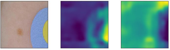
Under review as a conference paper at ICLR 2020

We create three variants of the SST dataset, each with different spurious signals which we aim to
ignore (examples in Sec S1). In the first variant, we add indicator words for each class (positive:
‘text’, negative: ‘video’) at a random location in each sentence. An unpenalized DNN will focus
only on those words, dropping to nearly random performance on the unbiased test set. In the second
variant, we use two semantically similar words (‘the’, ‘a’) to indicate the class by using one word
only in the positive and one only in the negative class. In the third case, we use ‘he’ and ‘she’ to
indicate class (example in Fig 5). Since these gendered words are only present in a small proportion
of the training dataset (∼ 2%), for this variant, we report accuracy only on the sentences in the test
set that do include the pronouns (performance on the test dataset not including the pronouns remains
unchanged). Table 4 shows the test accuracy for all datasets with and without CDEP. In all scenarios,
CDEP is successfully able to improve the test accuracy by ignoring the injected spurious signals.

Table 4: Results on SST. CDEP substantially improves predictive accuracy on the unbiased test set
after training on biased data.
                                               Unpenalized         CDEP
                           Random words          56.6 ± 5.8    75.4 ± 0.9
                           Biased (articles)     57.8 ± 0.8    68.2 ± 0.8
                           Biased (gender)       64.2 ± 3.1    78.0 ± 3.0

5   C ONCLUSION
In this work we introduce a novel method to penalize neural networks to align with prior knowledge.
Compared to previous work, CDEP is the first of its kind that can penalize complex features and
feature interactions. Furthermore, CDEP is more computationally efficient than previous work and
does not rely on backpropagation, enabling its use with more complex neural networks. We show
that CDEP can be used to remove bias and improve predictive accuracy on a variety of toy and
real data. The experiments here demonstrate a variety of ways to use CDEP to improve models
both on real and toy datasets. CDEP is quite versatile and can be used in many more areas to
incorporate the structure of domain knowledge (e.g. biology or physics). Of course, the effectiveness
of CDEP depends upon the quality of the prior knowledge used to determine the explanation targets.
Future work includes extending CDEP to more complex penalties, incorporating more fine-grained
explanations and interactions. We hope the work here will help push the field towards a more
rigorous way to use interpretability methods, a point which will become increasingly important as
interpretable machine learning develops as a field (Doshi-Velez & Kim, 2017; Murdoch et al., 2019).

R EFERENCES
Radhakrishna Achanta, Appu Shaji, Kevin Smith, Aurelien Lucchi, Pascal Fua, and Sabine
  Süsstrunk. Slic superpixels compared to state-of-the-art superpixel methods. IEEE transactions
  on pattern analysis and machine intelligence, 34(11):2274–2282, 2012.
Julius Adebayo, Justin Gilmer, Michael Muelly, Ian Goodfellow, Moritz Hardt, and Been Kim.
  Sanity checks for saliency maps. In Advances in Neural Information Processing Systems, pp.
  9505–9515, 2018.
Marco Ancona, Enea Ceolini, Cengiz Oztireli, and Markus Gross. Towards better understanding of
 gradient-based attribution methods for deep neural networks. In 6th International Conference on
 Learning Representations (ICLR 2018), 2018.
Sebastian Bach, Alexander Binder, Grégoire Montavon, Frederick Klauschen, Klaus-Robert Müller,
  and Wojciech Samek. On pixel-wise explanations for non-linear classifier decisions by layer-wise
  relevance propagation. PloS one, 10(7):e0130140, 2015.
David Baehrens, Timon Schroeter, Stefan Harmeling, Motoaki Kawanabe, Katja Hansen, and Klaus-
  Robert MÞller. How to explain individual classification decisions. Journal of Machine Learning
  Research, 11(Jun):1803–1831, 2010.

                                                  8
Under review as a conference paper at ICLR 2020

Tolga Bolukbasi, Kai-Wei Chang, James Y Zou, Venkatesh Saligrama, and Adam T Kalai. Man is
  to computer programmer as woman is to homemaker? debiasing word embeddings. In Advances
  in neural information processing systems, pp. 4349–4357, 2016.
Kaylee Burns, Lisa Anne Hendricks, Kate Saenko, Trevor Darrell, and Anna Rohrbach. Women
  also snowboard: Overcoming bias in captioning models. arXiv preprint arXiv:1803.09797, 2018.
Noel Codella, Veronica Rotemberg, Philipp Tschandl, M Emre Celebi, Stephen Dusza, David Gut-
  man, Brian Helba, Aadi Kalloo, Konstantinos Liopyris, Michael Marchetti, et al. Skin lesion
  analysis toward melanoma detection 2018: A challenge hosted by the international skin imaging
  collaboration (isic). arXiv preprint arXiv:1902.03368, 2019.
Piotr Dabkowski and Yarin Gal. Real time image saliency for black box classifiers. arXiv preprint
  arXiv:1705.07857, 2017.
Finale Doshi-Velez and Been Kim. Towards a rigorous science of interpretable machine learning.
  arXiv preprint arXiv:1702.08608, 2017.
Gabriel Erion, Joseph D Janizek, Pascal Sturmfels, Scott Lundberg, and Su-In Lee. Learning ex-
  plainable models using attribution priors. arXiv preprint arXiv:1906.10670, 2019.
Andre Esteva, Brett Kuprel, Roberto A Novoa, Justin Ko, Susan M Swetter, Helen M Blau, and
  Sebastian Thrun. Dermatologist-level classification of skin cancer with deep neural networks.
  Nature, 542(7639):115, 2017.
Ruth C Fong and Andrea Vedaldi. Interpretable explanations of black boxes by meaningful pertur-
  bation. arXiv preprint arXiv:1704.03296, 2017.
Nikhil Garg, Londa Schiebinger, Dan Jurafsky, and James Zou. Word embeddings quantify 100
  years of gender and ethnic stereotypes. Proceedings of the National Academy of Sciences, 115
  (16):E3635–E3644, 2018. ISSN 0027-8424. doi: 10.1073/pnas.1720347115. URL https:
  //www.pnas.org/content/115/16/E3635.
Robert Geirhos, Patricia Rubisch, Claudio Michaelis, Matthias Bethge, Felix A Wichmann, and
  Wieland Brendel. Imagenet-trained cnns are biased towards texture; increasing shape bias im-
  proves accuracy and robustness. arXiv preprint arXiv:1811.12231, 2018.
Sarthak Jain and Byron C Wallace. Attention is not explanation. arXiv preprint arXiv:1902.10186,
  2019.
Yann LeCun. The mnist database of handwritten digits. http://yann. lecun. com/exdb/mnist/, 1998.
Yi Li and Nuno Vasconcelos. Repair: Removing representation bias by dataset resampling. arXiv
  preprint arXiv:1904.07911, 2019.
Frederick Liu and Besim Avci. Incorporating priors with feature attribution on text classification.
  arXiv preprint arXiv:1906.08286, 2019.
Scott M Lundberg and Su-In Lee. A unified approach to interpreting model predictions. In Advances
  in Neural Information Processing Systems, pp. 4768–4777, 2017.
Masahiro Mitsuhara, Hiroshi Fukui, Yusuke Sakashita, Takanori Ogata, Tsubasa Hirakawa,
 Takayoshi Yamashita, and Hironobu Fujiyoshi. Embedding human knowledge in deep neural
 network via attention map. arXiv preprint arXiv:1905.03540, 2019.
W James Murdoch and Arthur Szlam. Automatic rule extraction from long short term memory
 networks. arXiv preprint arXiv:1702.02540, 2017.
W James Murdoch, Peter J Liu, and Bin Yu. Beyond word importance: Contextual decomposition
 to extract interactions from lstms. arXiv preprint arXiv:1801.05453, 2018.
W James Murdoch, Chandan Singh, Karl Kumbier, Reza Abbasi-Asl, and Bin Yu. Interpretable
 machine learning: definitions, methods, and applications. arXiv preprint arXiv:1901.04592, 2019.

                                                9
Under review as a conference paper at ICLR 2020

Weili Nie, Yang Zhang, and Ankit Patel. A theoretical explanation for perplexing behaviors of
 backpropagation-based visualizations. arXiv preprint arXiv:1805.07039, 2018.
Utku Ozbulak. Pytorch cnn visualizations.           https://github.com/utkuozbulak/
  pytorch-cnn-visualizations, 2019.
Marco Tulio Ribeiro, Sameer Singh, and Carlos Guestrin. Why should i trust you?: Explaining the
 predictions of any classifier. In Proceedings of the 22nd ACM SIGKDD International Conference
 on Knowledge Discovery and Data Mining, pp. 1135–1144. ACM, 2016.
Laura Rieger and Lars Kai Hansen. Aggregating explainability methods for neural networks stabi-
  lizes explanations. arXiv preprint arXiv:1903.00519, 2019.
Andrew Slavin Ross and Finale Doshi-Velez. Improving the adversarial robustness and interpretabil-
  ity of deep neural networks by regularizing their input gradients. In Thirty-second AAAI confer-
  ence on artificial intelligence, 2018.
Andrew Slavin Ross, Michael C Hughes, and Finale Doshi-Velez. Right for the right reasons: Train-
  ing differentiable models by constraining their explanations. arXiv preprint arXiv:1703.03717,
  2017.
Ramprasaath R Selvaraju, Michael Cogswell, Abhishek Das, Ramakrishna Vedantam, Devi Parikh,
  and Dhruv Batra. Grad-cam: Visual explanations from deep networks via gradient-based local-
  ization. See https://arxiv. org/abs/1610.02391 v3, 7(8), 2016.
Ramprasaath R Selvaraju, Michael Cogswell, Abhishek Das, Ramakrishna Vedantam, Devi Parikh,
  and Dhruv Batra. Grad-cam: Visual explanations from deep networks via gradient-based local-
  ization. In Proceedings of the IEEE International Conference on Computer Vision, pp. 618–626,
  2017.
Avanti Shrikumar, Peyton Greenside, Anna Shcherbina, and Anshul Kundaje. Not just a black
  box: Learning important features through propagating activation differences. arXiv preprint
  arXiv:1605.01713, 2016.
Karen Simonyan and Andrew Zisserman. Very deep convolutional networks for large-scale image
  recognition. arXiv preprint arXiv:1409.1556, 2014.
Chandan Singh, W James Murdoch, and Bin Yu. Hierarchical interpretations for neural network
  predictions. arXiv preprint arXiv:1806.05337, 2018.
Richard Socher, Alex Perelygin, Jean Wu, Jason Chuang, Christopher D Manning, Andrew Ng,
  and Christopher Potts. Recursive deep models for semantic compositionality over a sentiment
  treebank. In Proceedings of the 2013 conference on empirical methods in natural language pro-
  cessing, pp. 1631–1642, 2013.
Jost Tobias Springenberg, Alexey Dosovitskiy, Thomas Brox, and Martin Riedmiller. Striving for
  simplicity: The all convolutional net. arXiv preprint arXiv:1412.6806, 2014.
Julia Strout, Ye Zhang, and Raymond J Mooney. Do human rationales improve machine explana-
  tions? arXiv preprint arXiv:1905.13714, 2019.
Mukund Sundararajan, Ankur Taly, and Qiqi Yan. Axiomatic attribution for deep networks. ICML,
 2017.
Haohan Wang, Zexue He, Zachary C Lipton, and Eric P Xing. Learning robust representations by
  projecting superficial statistics out. arXiv preprint arXiv:1903.06256, 2019.
Julia K. Winkler, Christine Fink, Ferdinand Toberer, Alexander Enk, Teresa Deinlein, Rainer
  Hofmann-Wellenhof, Luc Thomas, Aimilios Lallas, Andreas Blum, Wilhelm Stolz, and Holger A.
  Haenssle. Association Between Surgical Skin Markings in Dermoscopic Images and Diagnostic
  Performance of a Deep Learning Convolutional Neural Network for Melanoma RecognitionSur-
  gical Skin Markings in Dermoscopic Images and Deep Learning Convolutional Neural Network
  Recognition of MelanomaSurgical Skin Markings in Dermoscopic Images and Deep Learning
  Convolutional Neural Network Recognition of Melanoma. JAMA Dermatology, 08 2019. ISSN

                                               10
Under review as a conference paper at ICLR 2020
2168-6068. doi: 10.1001/jamadermatol.2019.1735. URL https://doi.org/10.1001/
jamadermatol.2019.1735.
Omar Zaidan, Jason Eisner, and Christine Piatko. Using annotator rationales to improve machine
learning for text categorization. In Human Language Technologies 2007: The Conference of the
North American Chapter of the Association for Computational Linguistics; Proceedings of the
Main Conference, pp. 260–267, 2007.
Tianyuan Zhang and Zhanxing Zhu. Interpreting adversarially trained convolutional neural net-
works. arXiv preprint arXiv:1905.09797, 2019.
Luisa M Zintgraf, Taco S Cohen, Tameem Adel, and Max Welling. Visualizing deep neural network
decisions: Prediction difference analysis. arXiv preprint arXiv:1702.04595, 2017.
11Under review as a conference paper at ICLR 2020
Supplement
S1 A DDITIONAL DETAILS ABOUT SST TASK
Section 4.3 shows the results for CDEP on biased variants of the SST dataset. Here we show exam-
ples of the biased sentences (for task 2 and 3 we only show sentences where the bias was present) in
Figs. S1 to S3. For the first task, we insert two randomly chosen words in 100% of the sentences in
the positive and negative class respectively. We choose two words (“text” for the positive class and
“video” for the negative class) that were not otherwise present in the data set but had a representation
in Word2Vec.
Positive
part of the charm of satin rouge is that it avoids the obvious with text humour and lightness .
text a screenplay more ingeniously constructed than ‘memento’
good fun text, good action, good acting, good dialogue, good pace, good cinematography .
dramas like text this make it human .
Negative
... begins with promise, but runs aground after being video snared in its own tangled plot .
the video movie is well done, but slow .
this orange has some juice , but it 's video far from fresh-squeezed .
as it is, video it 's too long and unfocused .
Figure S1: Example sentences from the variant 1 of the biased SST dataset with decoy variables in
each sentence.
For the second task, we choose to replace two common words (”the” and ”a”) in sentences where
they appear (27% of the dataset). We replace the words such that one word only appears in the
positive class and the other world only in the negative class. By choosing words that are semantically
almost replaceable, we ensured that the normal sentence structure would not be broken such as with
the first task.
Positive
comes off as a touching , transcendent love story .
is most remarkable not because of its epic scope , but because of a startling intimacy
couldn't be better as a cruel but weirdly likable wasp matron
uses humor and a heartfelt conviction to tell that story about discovering your destination in
life
Negative
to creep the living hell out of you
holds its goodwill close , but is relatively slow to come to the point
it 's not the great monster movie .
consider the dvd rental instead
Figure S2: Example sentences from the variant 2 of the SST dataset with artificially induced bias on
articles (”the”, ”a”). Bias was only induced on the sentences where those articles were used (27%
of the dataset).
For the third task we repeat the same procedure with two words (“he” and “she”) that appeared in
only 2% of the dataset. This helps evaluate whether CDEP works even if the spurious signal appears
only in a small section of the data set.
12Under review as a conference paper at ICLR 2020
Positive
pacino is the best she's been in years and keener is marvelous
she showcases davies as a young woman of great charm , generosity and diplomacy
shows she 's back in form , with an astoundingly rich film .
proves once again that she's the best brush in the business
Negative
green ruins every single scene he's in, and the film, while it 's not completely wreaked, is
seriously compromised by that
i'm sorry to say that this should seal the deal - arnold is not, nor will he be, back .
this is sandler running on empty , repeating what he 's already done way too often .
so howard appears to have had free rein to be as pretentious as he wanted
Figure S3: Example sentences from the variant 3 of the SST dataset with artificially induced bias on
articles (”he”, ”she”). Bias was only induced on the sentences where those articles were used (2%
of the dataset).
S2 N ETWORK ARCHITECTURES AND TRAINING
S2.1 N ETWORK ARCHITECTURES
For the ISIC skin cancer task we used a pretrained VGG16 network retrieved from the PyTorch
model zoo. We use SGD as the optimizer with a learning rate of 0.01 and momentum of 0.9.
Preliminary experiments with Adam as the optimizer yielded poorer predictive performance.
or both MNIST tasks, we use a standard convolutional network with two convolutional channels
followed by max pooling respectively and two fully connected layers:
Conv(20,5,5) - MaxPool() - Conv(50,5,5) - MaxPool - FC(256) - FC(10). The models were trained
with Adam, using a weight decay of 0.001.
Penalizing explanations adds an additional hyperparameter, λ to the training. λ can either be set in
proportion to the normal training loss or at a fixed rate. In this paper we did the latter. We expect
that exploring the former could lead to a more stable training process. For all tasks λ was tested
across a wide range between [10−1 , 104 ].
The LSTM for the SST experiments consisted of two LSTM layers with 128 hidden units followed
by a fully connected layer.
S2.2 C OLOR MNIST
For fixing the bias in the ColorMNIST task, we sample pixels from the distribution of non-zero
pixels over the whole training set, as shown in Fig. S4
Figure S4: Sampling distribution for ColorMNIST
13Under review as a conference paper at ICLR 2020
Figure S5: Results on ColorMNIST (Test Accuracy). All averaged over thirty runs. CDEP is the
only method that captures and removes color bias.
For Expected Gradients we show results when sampling pixels as well as when penalizing the vari-
ance between attributions for the RGB channels (as recommended by the authors of EG) in Fig. S5.
Neither of them go above random accuracy, only achieving random accuracy when they are regular-
ized to a constant prediction.
S3 RUNTIME AND MEMORY REQUIREMENTS OF DIFFERENT ALGORITHMS
This section provides further details on runtime and memory requirements reported in Table S1.
We compared the runtime and memory requirements of the available regularization schemes when
implemented in Pytorch.
Memory usage and runtime were tested on the DecoyMNIST task with a batch size of 64. It is
expected that the exact ratios will change depending on the complexity of the used network and
batch size (since constant memory usage becomes disproportionally smaller with increasing batch
size).
The memory usage was read by recording the memory allocated by PyTorch. Since Expected Gra-
dients and RRR require two forward and backward passes, we only record the maximum memory
usage. We ran experiments on a single Titan X.
Table S1: Memory usage and run time were recorded for the DecoyMNIST task.
Unpenalized CDEP RRR Expected Gradients
Run time/epoch (seconds) 4.7 17.1 11.2 17.8
Maximum GPU RAM usage (GB) 0.027 0.068 0.046 0.046
S4 I MAGE SEGMENTATION FOR ISIC SKIN CANCER
To obtain the binary maps of the patches for the skin cancer task, we first segment the images using
SLIC, a common image-segmentation algorithm (Achanta et al., 2012). Since the patches look quite
distinct from the rest of the image, the patches are usually their own segment.
Subsequently we take the mean RGB and HSV values for all segments and filtered for segments
which the mean was substantially different from the typical caucasian skin tone. Since different
images were different from the typical skin color in different attributes, we filtered for those images
14Under review as a conference paper at ICLR 2020
recursively. As an example, in the image shown in Fig. S6, the patch has a much higher saturation
than the rest of the image. For each image we exported a map as seen in Fig. S6.
Figure S6: Sample segmentation for the ISIC task.
15Under review as a conference paper at ICLR 2020
S5 A DDITIONAL HEATMAP EXAMPLES FOR ISIC
We show additional examples from the test set of the skin cancer task in Figs. S7 and S8. We
see that the importance maps for the unregularized and regularized network are very similar for
cancerous images and non-cancerous images without patch. The patches are ignored by the network
regularized with CDEP.
Image Vanilla CDEP
Figure S7: Heatmaps for benign samples from ISIC
16Under review as a conference paper at ICLR 2020
Image Vanilla CDEP
Figure S8: Heatmaps for cancerous samples from ISIC
17Under review as a conference paper at ICLR 2020
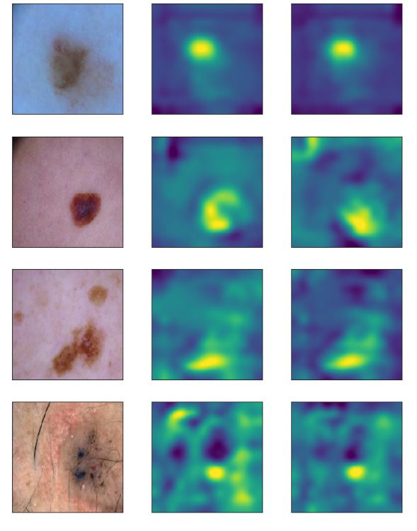
A different spurious correlation that we noticed was that proportionally more images showing skin
cancer will have a ruler next to the lesion. This is the case because doctors often want to show a
reference for size if they diagnosed that the lesion is cancerous. Even though the spurious correlation
is less pronounced (in a very rough cursory count, 13% of the cancerous and 5% of the benign images
contain some sort of measure), the networks learnt to recognize and exploit this spurious correlation.
This further highlights the need for CDEP, especially in medical settings.
Image Vanilla CDEP
Both networks learnt the
non-penalized spurious
correlation:
Ruler -> Cancer
Figure S9: Both networks learnt that proportionally more images with malignant lesions feature a
ruler next to the lesion. To make comparison easier, we visualize the heatmap by multiplying it with
the image. Visible regions are important for classification.
18You can also read