AIM 2020 Challenge on Efficient Super-Resolution: Methods and Results

AIM 2020 Challenge on Efficient
 Super-Resolution: Methods and Results

 Kai Zhang∗ , Martin Danelljan∗ , Yawei Li∗ , Radu Timofte∗ , Jie Liu, Jie Tang,
 Gangshan Wu, Yu Zhu, Xiangyu He, Wenjie Xu, Chenghua Li, Cong Leng, Jian
 Cheng, Guangyang Wu, Wenyi Wang, Xiaohong Liu, Hengyuan Zhao, Xiangtao
 Kong, Jingwen He, Yu Qiao, Chao Dong, Xiaotong Luo, Liang Chen, Jiangtao
arXiv:2009.06943v1 [eess.IV] 15 Sep 2020

 Zhang, Maitreya Suin, Kuldeep Purohit, A. N. Rajagopalan, Xiaochuan Li,
 Zhiqiang Lang, Jiangtao Nie, Wei Wei, Lei Zhang, Abdul Muqeet, Jiwon
 Hwang, Subin Yang, JungHeum Kang, Sung-Ho Bae, Yongwoo Kim, Liang
 Chen, Jiangtao Zhang, Xiaotong Luo, Yanyun Qu, Geun-Woo Jeon, Jun-Ho
 Choi, Jun-Hyuk Kim, Jong-Seok Lee, Steven Marty, Eric Marty, Dongliang
 Xiong, Siang Chen, Lin Zha, Jiande Jiang, Xinbo Gao, Wen Lu, Haicheng
 Wang, Vineeth Bhaskara, Alex Levinshtein, Stavros Tsogkas, Allan Jepson,
 Xiangzhen Kong, Tongtong Zhao, Shanshan Zhao, Hrishikesh P S, Densen
 Puthussery, Jiji C V, Nan Nan, Shuai Liu, Jie Cai, Zibo Meng, Jiaming Ding,
 Chiu Man Ho, Xuehui Wang, Qiong Yan, Yuzhi Zhao, Long Chen, Jiangtao
 Zhang, Xiaotong Luo, Liang Chen, Yanyun Qu, Long Sun, Wenhao Wang,
 Zhenbing Liu, Rushi Lan, Rao Muhammad Umer, and Christian Micheloni

 Abstract. This paper reviews the AIM 2020 challenge on efficient single
 image super-resolution with focus on the proposed solutions and results.
 The challenge task was to super-resolve an input image with a magnifica-
 tion factor ×4 based on a set of prior examples of low and corresponding
 high resolution images. The goal is to devise a network that reduces one
 or several aspects such as runtime, parameter count, FLOPs, activations,
 and memory consumption while at least maintaining PSNR of MSRRes-
 Net. The track had 150 registered participants, and 25 teams submitted
 the final results. They gauge the state-of-the-art in efficient single image
 super-resolution.

 1 Introduction
 Single image super-resolution (SR) aims at recovering a high-resolution (HR)
 image from a single degraded low-resolution (LR) image. Since the dawn of
 deep learning, this problem has been frequently tackled by researchers from
 low-level vision community with models based on convolutional neural networks
 (CNN) [9,22,43,23]. In order to strive towards the ultimate goal of deploying SR
 models for real-world applications, there exist a number of important research
 ∗
 K. Zhang (kai.zhang@vision.ee.ethz.ch, Computer Vision Lab, ETH Zurich), M.
 Danelljan, Y. Li and R. Timofte were the challenge organizers, while the other
 authors participated in the challenge. Appendix A contains the authors’ teams and
 affiliations. AIM webpage: https://data.vision.ee.ethz.ch/cvl/aim20/

2 K. Zhang et al.

directions. The most popular direction is to improve PSNR or the perceptual
quality, based on bicubic degradation assumption [47,59]. Significant achieve-
ments have been made on designing network architectures and training losses
for this purpose [23,50]. However, such bicubic degradation based methods would
give rise to poor performance if the real degradation deviates from the assumed
one [10]. Hence, another direction is to design a network to handle a more general
degradation with varying factors such as blur kernel [63,64,62,61]. In practical
applications, the blur kernel is usually unknown, thus some researchers attempt
to estimate the blur kernel of a given LR image for better reconstruction [3].
Such a strategy has also been successfully applied to the direction of SR with
unpaired data [35,36], where even more general degradation operations are con-
sidered. A recently emerging direction is to account for the ill-posed nature of
the SR problem by learning stochastic and explorable LR to HR mappings using
GAN [2,37] or Normalizing Flow based [34] approaches. This challenge report
focuses on another research direction, namely that of efficient SR, which is of
crucial importance in order to deploy models on resource-constrained devices.
 There are many factors that affect the efficiency of an SR network. Some
typical factors are runtime, the number of parameters, and floating point op-
erations (FLOPs). During past few years, several efficient SR works have been
proposed based on different techniques, including hand-designed network ar-
chitectures [9,22,65,18], network pruning [27], filter decomposition [25], network
quantization [33,28], neural architecture search (NAS) [30,4], and knowledge dis-
tillation [15,55]. Despite of significant achievements, these methods mostly focus
on the number of parameters and FLOPs. Recent works on high-level tasks have
pointed out that fewer FLOPs does not always indicate better network efficiency,
and the number of network activations is instead a more accurate measure of
the network efficiency [41]. As a result, efficient SR methods require a thorough
analysis from different aspects rather than only from the aspects of parameters
and FLOPs.
 Jointly with the Advances in Image Manipulation (AIM) 2020 workshop,
we organize the AIM Challenge on Efficient Super-Resolution. The task of the
challenge is to super-resolve an LR image to an HR image with a magnification
factor ×4 by a network that reduces one or several aspects such as runtime,
parameters, FLOPs, activations and memory consumption, while at least main-
taining PSNR of the baseline model. The challenge aims to seek advanced and
novel solutions for efficient SR, to benchmark their efficiency, and identify the
general trends.

2 AIM 2020 Efficient Super-Resolution Challenge

This challenge is one of the AIM 2020 associated challenges on: scene relight-
ing and illumination estimation [11], image extreme inpainting [40], learned
image signal processing pipeline [19], rendering realistic bokeh [20], real im-
age super-resolution [51], efficient super-resolution [58], video temporal super-
resolution [44] and video extreme super-resolution [12]. The objectives of this

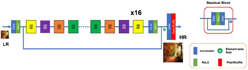
AIM 2020 Challenge on Efficient Super-Resolution 3

challenge are: (i) to advance research on efficient SR; (ii) to compare the effi-
ciency of different methods and (iii) to offer an opportunity for academic and
industrial attendees to interact and explore collaborations. This section details
the challenge itself.

2.1 DIV2K Dataset [1]

Following [1], the DIV2K dataset is adopted, which contains 1,000 DIVerse 2K
resolution RGB images. The HR DIV2K is divided into 800 training images, 100
validation images and 100 testing images. The corresponding LR DIV2K in this
challenge is the bicubicly downsampled counterpart with a down-scaling factor
×4. The testing HR images are hidden from the participants during the whole
challenge.

2.2 MSRResNet Baseline Model

The MSRResNet [50] serves as the reference SR model in this challenge. The
aim is to improve its efficiency while maintaining the SR performance. The
MSRResNet contains 16 residual blocks and a global identity skip connection is
adopted. Specifically, each residual block of MSRResNet consists of two 3 × 3
convolutional layers with Leaky ReLU activation in the middle and an identity
skip connection summed to its output, while the global identity skip connection
directly sums the bilinearly interpolated LR image to the output of final con-
volutional layer. The reference MSRResNet is trained on DIV2K [1], Flickr2K
and OST [49] datasets. The quantitative performance and efficiency metrics of
MSRResNet are given as follows. (1) The number of parameters is 1,517,571
(1.5M). (2) The average PSNRs on validation and testing sets of DIV2K are
29.00 dB and 28.70dB, respectively. (3) The average runtime over validation set
with PyTorch 1.5.1, CUDA Toolkit 10.2, cuDNN 7.6.2 and a single Titan Xp
GPU is 0.110 seconds. (4) The number of FLOPs for an input of size 256 × 256 is
166.36G. (5) The number of activations (i.e., elements of all outputs of convolu-
tional layers) for an input of size 256 × 256 is 292.55M. (5) The maximum GPU
memory consumption for an input of size 256 × 256 is 610M. (6) The number of
convolutional layers is 37.

2.3 Competition

The aim of this challenge is to devise a network that reduces one or several
aspects such as runtime, parameters, FLOPs, activations and memory consump-
tion while at least maintaining the PSNR of MSRResNet.
Challenge phases (1) Development and validation phase: The participants
had access to the 800 LR/HR training image pairs and 100 LR validation im-
ages of the DIV2K dataset. The participants were also provided the reference
MSRResNet model from github (https://github.com/znsc/MSRResNet), al-
lowing them to benchmark its runtime on their system, and to adopt it as a

4 K. Zhang et al.

baseline if desired. The participants could upload the HR validation results on
the evaluation server to measure the PSNR of their model to get immediate feed-
back. The number of parameters and runtime was computed by the participant.
(2) Testing phase: In the final test phase, the participants recieved access to the
100 LR testing images. The participants then submitted their super-resolved re-
sults to the Codalab evaluation server and e-mailed the code and factsheet to
the organizers. The organizers verified and ran the provided code to obtain the
final results. Finally, the participants received the final results at the end of the
challenge.
Evaluation protocol The quantitative evaluation metrics includes valida-
tion and testing PSNRs, runtime, number of parameters, number of FLOPs,
number of activations, and maximum GPU memory consumed during infer-
ence. The PSNR was measured by first discarding the 4-pixel boundary around
the images. The runtime is averaged over the 100 LR validation images and
the best one among three consecutive trails is selected as the final result. The
FLOPs, activations, and memory consumption are evaluated on an input im-
age of size 256 × 256. Among the above metrics, the runtime is regarded as the
most important one. The validation and testing PSNRs should be at least on
par with the baseline. A code example for calculating these metrics is available
at https://github.com/cszn/KAIR/blob/master/main_challenge_sr.py.

3 Challenge Results

Table 1 reports the final test results and rankings of the teams. The solutions
with lower validation PSNR than the MSRResNet baseline are not ranked. In
addition, the solutions by lyl, LMSR, CET CVLab and wozhu teams are not
ranked due to the lack of experimental verification by the organizers. The results
of the overall first place winner team in AIM 2019 constrained SR challenge [60]
are also reported for comparison. The methods evaluated in Table 1 are briefly
described in Sec. 4 and the team members are listed in Appendix A.
 According to Table 1, we can have the following observations. First, the
NJU MCG team is the overall first place winner of this challenge, while AiriA CG
and UESTC-MediaLab win the overall second place and overall third place, re-
spectively. Second, NJU MCG and AiriA CG produce the best runtime; XPixel
is the first place winner for the number of parameters; SC-CVLab, NJU MCG
and MLVC are the top-3 teams that achieve similar performance on FLOPs;
NJU MCG and AiriA CG are the first two place winners for the number of acti-
vations; MLVC achieves the best performance for memory consumption. Third,
MLVC and SC-CVLAB are superior in the number of parameters and the num-
ber of FLOPs but fail to get a matched runtime. On the other hand, although
the methods proposed by 404NotFound and MLVC have lower parameters and
FLOPs than IMDN, they exhibit a much slower runtime. To analyze such dis-
crepancies, we report the Spearman rank-order correlation coefficient (SROCC)
values of the number of parameters, the number of FLOPs, the number of ac-
tivations, and maximum GPU memory consumption with respect to runtime in

AIM 2020 Challenge on Efficient Super-Resolution 5

Table 1. Results of AIM 2020 efficient SR challenge. ‘*’ means the organizers did not
verify the results. ‘Runtime’ is tested on validation datasets, the average image size is
421×421. ‘#Params’ denotes the total number of parameters. ‘FLOPs’ is the abbrevi-
ation for floating point operations. ‘#Activations’ measures the number of elements of
all outputs of convolutional layers. ‘Memory’ represents maximum GPU memory con-
sumption according to the PyTorch function torch.cuda.max memory allocated().
‘#Conv’ represents the number of convolutional layers. ‘FLOPs’, ‘#Activations’, and
‘Memory’ are tested on an LR image of size 256×256. This is not a challenge for
PSNR improvement. The ‘validation/testing PSNR’ and ‘#Conv’ are not
ranked.
 PSNR PSNR Runtime #Params #FLOPs #Activations Memory Extra
Team Author #Conv
 [Val.] [Test] [Val.] [s] [M] [G] [M] [M] Data
NJU MCG TinyJie 29.04 28.75 0.037(1) 0.433(3) 27.10(2) 112.03(1) 200(4) 64 Yes
AiriA CG Now 29.00 28.70 0.037(1) 0.687(10) 44.98(9) 118.49(2) 168(3) 33 Yes
UESTC-MediaLab Mulns 29.01 28.70 0.060(4) 0.461(5) 30.06(4) 219.61(10) 146(2) 57 Yes
XPixel zzzhy 29.01 28.70 0.066(6) 0.272(1) 32.19(6) 270.53(12) 311(8) 121 Yes
HaiYun Sudo 29.09 28.78 0.058(3) 0.777(13) 49.67(10) 132.31(4) 225(5) 104 Yes
IPCV IITM ms ipcv 29.10 28.68 0.064(5) 0.761(12) 50.85(11) 130.41(3) 229(6) 59 Yes
404NotFound xiaochuanLi 29.01 28.70 0.073(9) 0.599(8) 39.36(7) 170.06(6) 271(7) 90 Yes
MDISL-lab ppplang 29.01 28.68 0.067(7) 0.660(9) 42.40(8) 149.09(5) 516(12) 61 Yes
MLVC ysb 29.00 28.72 0.104(11) 0.441(4) 27.11(3) 212.24(9) 112(1) 159 No
XMUlab SuckChen 29.00 28.77 0.078(10) 0.691(11) 53.62(12) 184.74(7) 468(10) 72 No
MCML-Yonsei GWJ 29.01 28.66 0.070(8) 1.289(15) 84.43(14) 188.74(8) 798(16) 68 Yes
LMSR martyste 29.00 28.71 0.081∗(11) 1.126∗(14) 75.72∗(14) ∗
 158.33(6) ∗
 192(4) 31* Yes
ZJUESR2020 BearMaxZJU 29.04 28.74 0.105(12) 0.516(6) 54.38(13) 225.44(11) 594(13) 42 Yes
SC-CVLAB chensa 29.01 28.72 0.157 0.353(2) 26.96(1) 302.30(13) 595(15) 91 Yes
HiImageTeam HiImageTeam 29.01 28.68 0.153 0.530(7) 90.11(15) 325.05(14) 378(9) 101 Yes
SAMSUNG TOR AIC hcwang 28.98 28.71 0.240 0.558(8) 31.88(5) 576.45(16) 477(11) 59 Yes
neptuneai neptuneai 29.14 28.84 0.217 1.227(14) 147.72(16) 535.82(15) 597(15) 45 *
lyl tongtong 29.44 29.13 * 0.408* * * * 128* No
CET CVLab hrishikeshps 29.00 28.74 5.00 1.378* * * * * Yes
wozhu wozhu 28.98 * * 0.720* * * * * Yes
 The following 5 methods are not ranked since their validation/testing PSNRs are not on par with the baseline.
InnoPeak SR qiuzhangTiTi 28.93 28.60 0.053 0.361 81.72 145.75 66 35 Yes
Summer sysu wxh 28.87 28.54 0.043 0.488 31.82 125.30 227 35 No
Zhang9678 Zhang9678 28.78 28.50 * 0.664* 48.08* * * 36* No
H-ZnCa suen 28.69 28.42 0.045 0.364 32.01 170.45 299 67 No
MLP SR raoumer 27.89 27.77 1.313 0.047 50.66* 351.27* 1064 10* Yes
Winner AIM19 IMDN 29.13 28.78 0.050 0.893 58.53 154.14 120 43 Yes
Baseline MSRResNet 29.00 28.70 0.114 1.517 166.36 292.55 610 37 Yes

Table 2. Spearman rank-order correlation coefficient (SROCC) values of #Params,
#FLOPs, #Activations, Memory with respect to runtime.

 Metric #Params #FLOPs #Activations Memory
 SROCC 0.1734 0.2397 0.8737 0.6671

Table 2. Note that SROCC is widely used to measure the prediction monotonic-
ity of a metric and a better metric tends to have a higher SROCC. It can be
seen from Table 2 that the number of parameters and the number of FLOPs
do not correlate well with the runtime. Instead, the number of activations is a
better metric. Such a phenomenon has also been reported in [41]. Note that the
number of parameters and the number of FLOPs are still important aspects of
model efficiency.

6 K. Zhang et al.

3.1 Architectures and main ideas

Various techniques are proposed to improve the efficiency of MSRResNet and
IMDN. Some typical techniques are given in the following.

1. Modifying the information multi-distillation block of IMDN. The
 overall first place winner NJU MCG proposed an efficient residual feature
 distillation block (RFDB) by incorporating shallow residual connection and
 enhanced spatial attention (ESA) module, using 1×1 convolutions for feature
 distillation, and reducing the number of channels from 64 to 50. AiRiA CG
 proposed to reduce IMDB blocks and adopt converted asymmetric convolu-
 tion to improve the efficiency. Inspired by IMDB and IdleBlock, ZJUESR2020
 proposed multi-scale IdleBlock.
2. Changing the upsampling block. Instead of achieve a upscaling factor of
 4 via two successive ‘PixelShuffle(×2)→Conv→Leaky ReLU’ as in MSRRes-
 Net, XPixel proposed to replace the PixelShuffle layer with nearest neighbor
 interpolation layer, while most of the other methods, such as NJU MCG,
 AiRiA CG, HaiYun and IPCV IITM, proposed to directly reconstruct the
 HR image via a single PixelShuffle(×4) layer.
3. Adopting global feature aggregation. In contrast to the local feature
 aggregation strategy of IMDN, a global feature aggregation strategy which
 concatenates the features of different blocks is adopted in several teams
 such as NJU MCG, Haiyun, IPCV IITM and 404NotFound. As a typical
 example, NJU MCG proposed to concatenate the outputs of 4 RFDB blocks,
 then use a 1 × 1 convolutional layer for feature reduction and finally adopt
 ‘Conv3×3→PixelShuffle(×4)’ to produce the HR image.
4. Incorporating attention module. NJU MCG proposed to insert enhanced
 spatial attention module into the RFDB block. Xpixel proposed pixel atten-
 tion to produce 3D attention maps. MLVC proposed multi-attention block
 based on enhanced spatial attention (ESA) and cost-efficient attention (CEA).
5. Reducing the number of parameters by recursive layers. Zhang9678
 proposed to adopt LSTM to reduce parameters, while InnoPeak SR proposed
 recursive residual blocks.
6. Applying network pruning. SC-CVLAB proposed a fine-grained chan-
 nel pruning strategy to get a lightweight model from an over-parameterized
 hybrid composition based SR network.
7. Replacing the basic residual block of MSRResNet with new block.
 Xpixel proposed self-calibrated convolution block with pixel attention. 404Not-
 Found proposed to replace the normal 3 × 3 convolution with Ghost con-
 volution and 1 × 3 convolution. SAMSUNG TOR AIC proposed modified
 MobileNetV3 block.

3.2 Fairness

There are some fair and unfair tricks to improve the validation and testing
PSNRs for this challenge. On one hand, using additional training data is fair

AIM 2020 Challenge on Efficient Super-Resolution 7

since the MSRResNet baseline was trained on DIV2K [1], Flickr2K [46] and
OST [49] datasets. Most of the teams used the provided DIV2K and additional
Flickr2K for training. In addition, using advanced data augmentation strategy
during training is also a fair trick. On the other hand, it is unfair to train
the model with the validation LR images, validation HR images, and testing LR
images. First, training on LR/HR validation images would improve the validation
PSNR. Second, it tends to get a PSNR gain if the model is trained on pairs of LR
images and their downsampled counterparts. Third, the PSNR can be improved
by knowledge distillation technique on validation and testing LR images.

3.3 Conclusions
From the above analysis of different solutions, we can have several conclusions.
(i) The proposed methods improve the state-of-the-art for efficient SR. Com-
pared to the first place method IMDN in AIM 2019 constrained SR challenge,
NJU MCG team’s method provides a significant gain with respect to the run-
time, parameters, FLOPs, and activations. (ii) The number of FLOPs and the
number of parameters do not correlate well with network efficiency. In compar-
ison, the number of activations is a more proper metric. (iii) All of the overall
top-6 methods employ hand-designed network architecture. The effectiveness of
network pruning, knowledge distillation, network quantization and NAS for this
efficient SR challenge requires further study. (iv) Future work on efficient SR
should take runtime, parameters, FLOPs, and activations into consideration.

4 Challenge Methods and Teams
NJU MCG
The NJU MCG proposed Residual Feature Distillation Network (RFDN)
for fast and lightweight image SR [31]. The proposed RFDN is inspired by two
recent works IMDN [18] and RFANet [32]. As shown in Fig. 1(a), the main
part of information distillation block (IMDB) is a progressive refinement module
(PRM) marked with a gray background. Although PRM achieves prominent
improvements, it is not efficient enough and introduces some inflexibility because
of the channel splitting operation. The distilled features are generated by 3 × 3
convolution filters that have many redundant parameters. Moreover, the feature
refinement pipeline (along the right branch of the PRM) is coupled together with
channel splitting operation so that it is hard to use identity connections only
for this pipeline. The IMDB-R in Fig. 1(b) solves these problems by replacing
the channel splitting operation with two concurrent 3 × 3 convolutions. It is
more flexible than the original IMDB. Based on this new architecture, RFDB in
Fig. 1(c) uses three 1 × 1 convolutions for feature distillation. Furthermore, it
uses the shallow residual block (SRB) in Fig. 1(d) as the feature extractor which
can benefit most from the residual learning strategy. For shallow SR models, it is
more efficient to use spatial attention than channel attention. So RFDB replaces
the CCA layer with the ESA block in RFANet [32].

8 K. Zhang et al.

 The proposed RFDN model contains 4 RFDBs, the overall framework follows
the pipeline of IMDN, where global feature aggregation is used to augment the
final features and the number of feature channels is set to 50. During the training
of RFDN, HR patches of size 256 × 256 are randomly cropped from HR images,
and the mini-batch size is set to 64. The RFDN model is trained by minimizing
L1 loss function with Adam optimizer. The initial learning rate is set to 5 × 10−4
and halved at every 200 epochs. After 1000 epochs, L2 loss is used for fine-tuning
with learning rate of 1×10−5 . DIV2K and Flickr2K datasets are used for training
the RFDN model.

 Conv-3
 Conv-3 Conv-3 Conv-1 SRB
 Channel Split

 Conv-3
 Conv-3 Conv-3 Conv-1 SRB

 Channel Split

 Conv-3
 Conv-3 Conv-3 Conv-1 SRB

 Channel Split

 Conv-3 Conv-3
 Conv-3

 Concat Concat Concat

 CCA Layer 64 CCA Layer 64 Conv-1 Conv-3
 48 48
 Conv-1 Conv-1 CCA Layer
 16 16
 ReLU

 (a) (b) (c) (d)

Fig. 1. NJU MCG Team: (a) IMDB: the original information multi-distillation block.
(b) IMDB-R: rethinking of the IMDB. (c) RFDB: residual feature distillation block.
(d) SRB: shallow residual block.

AiRiA CG

The AiRiA CG team proposed Faster Information Multi-Distillation Net-
work via Asymmetric Convolution (FIMDN). The proposed FIMDN shown
in Fig. 2 is modified from IMDN [18] with minor improvements such as less build-
ing blocks and converted asymmetric convolution. Different from IMDN, FIMDN
only uses 6 CACBs as the building blocks to further accelerate the network. As
illustrated in Fig. 3, FIMDN employs four ‘Conv-3’ layers and retains a part of
the information step-by-step. Then the hierarchical features are fused by using
a 1 × 1 convolution layer. In particular, inspired by ACNet [8], FIMDN utilizes
the original AC model where 3 × 3 convolution layer is coupled with parallel

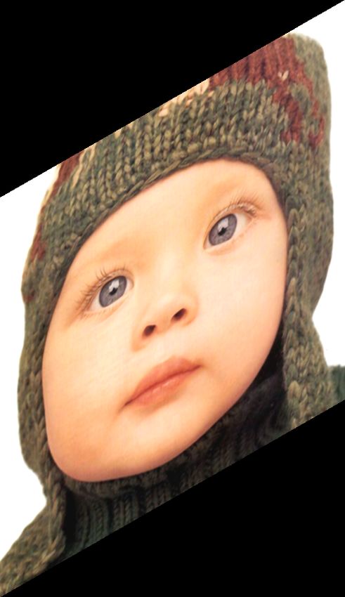
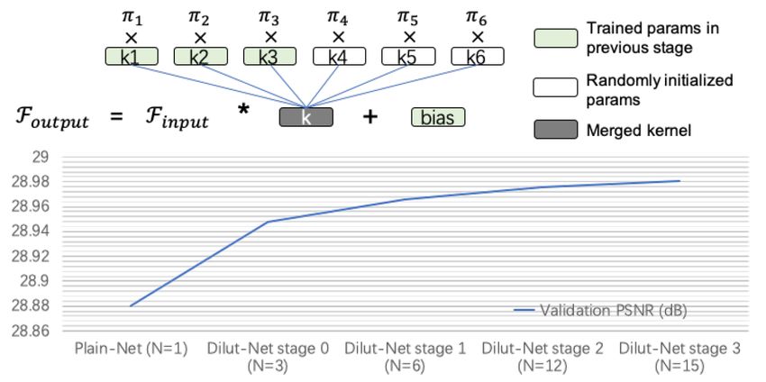
AIM 2020 Challenge on Efficient Super-Resolution 9

1 × 3, 3 × 1 kernels. After the first training stage, the original AC model is con-
verted into a single standard 3 × 3 convolution layer. Fig. 3 illustrates the fusion
process. The training process contains two stages with four steps.

 1. At the first stage, the original AC model is equipped with three parallel
 asymmetric convolutions.
 I. Pre-training on DIV2K+Flickr2K (DF2K). HR patches of size 256 × 256
 are randomly cropped from HR images, and the mini-batch size is set to
 64. The original FIMDN model is trained by minimizing L1 loss function
 with Adam optimizer. The initial learning rate is set to 2e-4 and halved
 at every 3600 epochs. The total number of epochs is 18000.
 II. Fine-tuning on DF2K. HR patch size and the mini-batch size are set
 to 640 × 640 and 24, respectively. The FIMDN model is fine-tuned by
 minimizing L2 loss function. The initial learning rate is set to 1e-5 and
 halved at every 720 epochs. The total number of epochs is 3600.
 III. Fine-tuning on DIV2K. HR patch size and the mini-batch size are set
 to 640 × 640 and 4, respectively. The FIMDN model is finetuned by
 minimizing L2 loss function. The initial learning rate is set to 1e-6 and
 halved at every 400 epochs. The total number of epochs is 2000.
 2. At the second stage, the final FIMDN model is obtained by converting three
 parallel convolutional kernels into a single 3 × 3 convolution layer.
 IV. Fine-tuning on DIV2K. HR patch size is set to 640 × 640 and the mini-
 batch size is set to 24. The final CAC model is fine-tuned by minimizing
 L2 loss function. The initial learning rate is set to 1e-6 and halved at
 every 200 epochs. The total number of epochs is 1000.

 Fig. 2. AiRiA CG Team: architecture of FIMDN.

UESTC-MediaLab

The UESTC-MediaLab team proposed a novel training strategy which is able
to boost the performance of CNNs without extra parameters. The traditional
convolution layer can be formulated as Foutput = Finput ∗ k̃ + b. The team
 P
decomposed the kernel k̃ into N kernel bases, i.e., k̃ = i πi × ki , where

10 K. Zhang et al.

Fig. 3. AiRiA CG Team: Left: Detailed architecture of FIMDN. “Conv-1” denotes the
1 × 1 convlution layer. 64, 48, and 16 represent the number of output channels. Right:
Details of the asymmetric 3 × 3 convolution. “CAC” means converted Asymmetric
Convolution (CAC).

{πi |i = 1, 2, . . . , N } are trainable merging weights [25]. The proposed train-
ing procedure has multiple stages. At the first stage (denoted as 0-th stage),
the model is trained from scratch with the number of kernel bases N0 = 3 in
each layer. All kernel bases are initialized randomly with Xavier-Uniform [13],
merging weights with N10 and bias with zeros. At the t-th (t ≥ 1) stage, δt kernel
bases in each layer which are added and randomly initialized, and the merge
weights are initialized with N1t where Nt = Nt−1 + δt . Each training stage termi-
nates when the validation loss converges. After the training phase, only merged
kernels k̃ and the bias b are saved. The kernel bases ki and merging weights πi
are not necessary in the inference phase. As shown in Fig. 4, the performance
increases gradually with the number of kernel bases in Dilut-Net (the network
trained with the proposed strategy). The Plain-Net denotes the network using
traditional convolutional layers without kernel bases.

 As for the model structure, the UESTC-MediaLab team modified the struc-
ture of IMDN [18] from the following aspects. Firstly, the computing unit ‘conv3×3
→ LeakyRelu’ is replaced by ‘gconv3×3 → PRelu → conv1×1’, where gconv
denotes the group convolution which doubles the number of feature maps. Sec-
ondly, adaptive skip-connection is adopted in the model, which parameterizes the
connection relationship between the outputs of blocks. Thirdly, the depth and
width of the network is modified to achieve a better balance between efficiency
and effectiveness.

AIM 2020 Challenge on Efficient Super-Resolution 11

Fig. 4. UESTC-MediaLab Team: kernel dilution and performance of different training
stages.

XPixel
The XPixel team proposed a simple yet efficient network called Pixel
Attention Network (PAN) [66], which achieves the same performance as
MSRResNet with only 272,419 parameters. The main contribution is “Pixel At-
tention” scheme. The framework consists of three stages depicted in Fig. 5. First,
one convolution layer extracts the features, then 16 SC-PA blocks are utilized for
non-linear mapping, at last there are two U-PA blocks for final reconstruction.
Pixel attention is adopted in the SC-PA and U-PA blocks. Next, the details of
these new modules will be described.
 Pixel Attention. First, let us revisit channel attention [17] and spatial
attention [42]. Channel attention aims to obtain 1D (C × 1 × 1) attention feature
vector, while spatial attention obtains a 2D (1 × H × W ) attention map. Note
that C is the number of channels, H and W are the height and width of the
features, respectively. Different from them, proposed pixel attention is able to
generate a 3D (C × H × W ) matrix as the attention features. As shown in Fig. 5,
pixel attention only uses a 1 × 1 convolution layer and a sigmoid function to
obtain the attention maps which will then be multiplied with the input features.
 SC-PA Block. The main block in the network is called Self-Calibrated
convolution with Pixel Attention (SC-PA). Specifically, proposed pixel attention
scheme is added to the Self-Calibrated convolution module. Basically, SC-PA is
comprised of two branches. Each branch contains a 1 × 1 convolution layer at
the beginning, which will reduce half of the channel number. The upper branch
also contains two 3 × 3 convolution layers, where the first one is equipped with
a PA module. This branch transforms X1 to Y1 . In the second branch, only a
single 3×3 convolution layer is used to generate Y2 since the original information
should be maintained. Finally, Y1 and Y2 are concatenated into Y3 , which will
then be passed to a 1 × 1 convolution layer. In order to accelerate training,
shortcut is used to produce the final output features Y .
 U-PA Block. Except for the main blocks, pixel attention is also adopted in
the final reconstruction stage. Specifically, proposed U-PA block is added after
each upsampling layer. Note that in previous SR networks, a reconstruction stage
is basically comprised of upsampling and convolution layers. Besides, plenty of

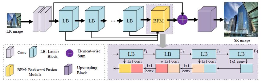
12 K. Zhang et al.

SR networks (e.g. MSRResNet) use PixelShuffle layer to upsample the features,
which is computational expensive. To reduce the computation cost and param-
eters in the reconstruction stage, Nearest Neighbor interpolation layer is used
to replace the PixelShuffle layer and the following convolution layer will reduce
the number of channels by half. Moreover, previous works have shown that at-
tention mechanism can effectively improve the performance in SR tasks but few
researchers investigate it in the upsampling stage. In this work, the U-PA block
is introduced after each upsampling layers. As shown in Fig. 5, the U-PA block
consists of a PA layer between two convolution layers. Experiments have been
conducted to demonstrate its effectiveness.
 Implementation details. During training, DIV2K and Flickr2K are uesd
as training datasets. The HR patch size is set to 256 × 256. The batch size is
set to 32. L1 loss function is adopted with Adam optimizer to train the model.
During validation, the model achieves an average PSNR of 29.00 dB on DIV2K
validation dataset. The inference time is about 0.0758s per image with a single
GTX 1080Ti GPU.

 Fig. 5. XPixel Team: the network architecture.

HaiYun

The HaiYun team proposed a lightweight SR network (see Fig. 6). Due to the
frequent use of residual block (RB) in SR models, they pursue an economical
structure to adaptively combine RBs. Inspired by lattice filter bank, a lattice
block (LB) is designed where two butterfly structures are applied to combine
two RBs. LB has the potential of various linear combinations of two RBs. Each
case of LB depends on the combination coefficients which are determined by the
attention mechanism. LB favors the lightweight SR model with the reduction of
about half amount of the parameters while keeping the similar SR performance.
Moreover, a lightweight SR model, i.e., LatticeNet, is proposed, which uses a
series of LBs and the backward feature fusion.

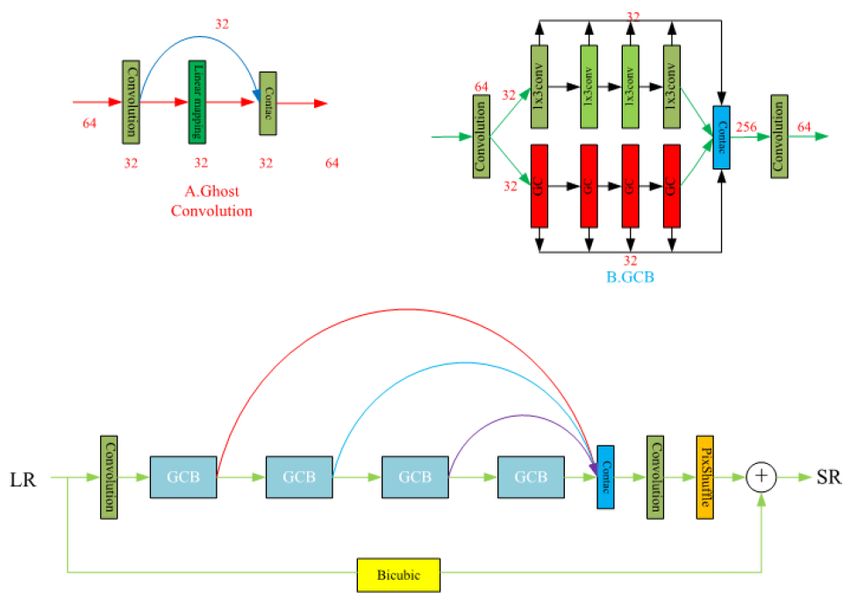
AIM 2020 Challenge on Efficient Super-Resolution 13

 Fig. 6. HaiYun Team: the network architecture.

IPCV IITM
The IPCV IITM team proposed to stack multiple residual blocks for grad-
ual feature refinement. One 3 × 3 convolution with 64 output channels is
used to extract features from the LR image. Multiple residual blocks are stacked
together and at the end all intermediate feature maps are fused by a 1 × 1 convo-
lution layer. As shown in Fig. 7, residual blocks perform channel split operation
on the preceding features, producing two feature splits. One is preserved and the
other portion is fed into the next calculation unit. The retained part is used as
the refined features. Each convolutional operation is followed by a Leaky ReLU
activation function except for the last 1 × 1 convolution. Two sub-networks are
used for predicting spatial and channel attention map to perform feature-wise
gating operation on the features. For the purpose of faster inference, the gating
function is used in alternating residual blocks as indicated in the figure. Given a
feature map of size C × H × W , the spatial and channel attention module pro-
duces H × W and C dimensional soft gates, which are element-wise multiplied
with the feature. The same sub-networks are used for all the residual blocks to
reduce the number of parameters. At the end, the gated feature is added to the
input. The up-sampler at the end of the network includes one 3 × 3 convolution
and a sub-pixel convolution.

404NotFound
The 404NotFound team proposed GCSR which includes three main parts (see
Fig. 8). Firstly, the input channels are divided into 2 parts. Ghost convolution
and 1 × 3 convolution are adopted to replace normal convolution. Secondly, a
special loss is proposed which consists of L1 loss for low frequency information
reconstruction and gradient loss for high-frequency information reconstruction.
Thirdly, bicubic upscaling for the LR image is used.

MDISL-lab
The MDISL-lab team proposed PFSNet. The main idea is to keep the width
of features in an SR network by making full use of a shared feature in every
block for efficient SR. In details, the MDISL-lab team found that keeping the

14 K. Zhang et al.

 Fig. 7. IPCV IITM Team: the network architecture.

 Fig. 8. 404NotFound Team: the network architecture.

width of features is necessary for the high performance of SR networks. And
there are many redundancy in feature maps of SR networks. Thus, a series of
cheap operations with cheap cost are applied to a shared feature to generate
many simple features. These simple features are then concatenated with some
normal features at the channel dimension and fed to convolutional layers. In this
way, the width of output feature of most convolutional layers could be reduced,

AIM 2020 Challenge on Efficient Super-Resolution 15

thus reducing the computational cost. Meanwhile, the width of input features
could still be maintained by the shared feature followed by cheap operations.
 The architecture of PFSNet is shown in Fig. 9. First, the Feautre Share
Block (FSB) is constructed by several 3 × 3 convolutional layers, a shared 3 × 3
convolutional layer, several cheap operations. And a 1 × 1 convolutional layer
is used to reduce the number of feature channels. The ⊕ symbol in the figure
represents concatenation at channel dimension. All 3 × 3 convolutional layers
output features with 32 channels while the input features of all convolutional
layers has 64 channels.

 Fig. 9. MDISL-lab Team: the network architecture.

MLVC
The MLVC proposed Multi-Attentive Feature Fusion Super-Resolution
Network (MAFFSRN) [38]. The main architecture shown in Fig. 10 is based
on RDN [65] that consists of local and global blocks. The feature fusion group
(FFG) and multi-attention block (MAB) are used as global and local blocks, re-
spectively. The MAB is inspired by enhanced spatial attention (ESA) [32]. MAB
introduces another cost-efficient attention mechanism (CEA) [5] to refine the
input features. The CEA basically consists of point-wise and depth-wise con-
volutions. It is incorporated into the MAB block to improve the performance
of the network with negligible additional computational cost. Furthermore, it
is observed that the original ESA block is computationally expensive due to
convolutional group. Thus, the convolutional group is replaced by dilated convo-
lutions with different dilated factors. Lastly, element-wise addition is performed
between the output of dilated convolutions to avoid the grid effects [57]. FFG is
composed of a stack of MAB which are combined using binarized feature fusion
(BFF) [39].

16 K. Zhang et al.

 Upsample
 10

 P Shuffle
 Conv (5)
 Conv (3)
 FFG1 FFGn-2 FFGn-1 FFGn
 02

 P Shuffle
 Conv (3)
 LR

 HR

 CEA
 MAB1

 Conv (1)

 Sigmoid
 DW (5)
 C Shuffle

 Conv (1)
 concat

 DConv (3)
 MABm-2

 SConv (3)

 Upsample
 MaxPool
 Conv (3)

 Conv (3)

 Conv (1)

 Conv (1)

 Sigmoid
 2
 MABm-1 1 

 DConv (3)
 MABm

Fig. 10. MLVC Team: the network architecture. The top image represents the whole
structure of proposed model, bottom left represents structure of feature fusion group
(FFG), and bottom right shows structure of multi-attention block (MAB).

XMUlab
The XMUlab team proposed PixelShuffle Attention Network. As shown in
Fig. 11, the network contains several gated fusion groups. Each group has 4
residual blocks. Unlike the common use of attention module, PixelShuffle at-
tention Network applies spatial attention and channel attention to the upscaled
feature. Gated fusion group gather the output features from previous groups.
The channel number in the network is reduced from 64 to 32 compared with
other methods, which enables the network goes deeper. The LR image is also
concatenated with feature map to extract more information.

MCML-Yonsei
The MCML-Yonsei proposed LarvaNet: Hierarchical Super-Resolution via
Multi-exit Architecture [21] (see Fig. 12). The main idea of the proposed
LarvaNet is to divide a network into some body modules and to make each
body module to generate an output SR image. This is inspired by the fact that
MSRResNet is effective for generating residual contents which is added to the
image interpolated from the LR image. In their experiment, using interpolation
increases PSNR by about 0.2 dB compared to the MSRResNet model without
interpolation. Like MSRResNet generates residual contents to be added with a
interpolated image, each body module of LarvaNet generates residual contents
to be added with the previous modules output image. With this idea, the model
can learn features important for SR at early stages, and can generate a more
accurate SR image because of the accumulation of residual information.

AIM 2020 Challenge on Efficient Super-Resolution 17

 Upscale-1

 GFG-G +
 GFG-1 GFG-d
 F0 Fg-1 Fg FG

 I LR Upscale-2 I HR

 Initial Feature Deep Feature Extraction HR Image
 Extraction and Fusion Reconstruction

 F0
 Conv Gated +
 Layer fusion Element-wise
 LFB-b group Sum

 LFB-B
 LFB-1

 Fg-1 +
 Pixelshuffle- Concate
 Sub-pixel
 Attention
 I LR
 I LR (a) (b)

 Fig. 11. XMUlab Team: the network architecture.

 In order to search for an optimal base architecture, they investigate extensive
variations of the baseline MSRResNet model in terms of the numbers of channels
and blocks, upsampling methods, interpolation methods, weight initialization
methods, and activation functions. Following the results of the investigating
experiments, they used a MSRResNet with best settings as base architecture of
the multi-exit architecture, LarvaNet. The overall architecture of LarvaNet is
illustrated in Fig. 12. Each body module consisting of residual blocks generates
features and the previous features are accumulated by skip connection. A sub-
module is appended to the body module. It generates an SR output image using
features from the body module and interpolated SR image. The tail module takes
all the features generated by the body modules and concatenates the features,
and generates a final output image. The average of all the losses from the early
and final output images is considered as the loss function of training the model.

 Fig. 12. MCML-Yonsei Team: the network architecture.

18 K. Zhang et al.

LMSR
LMSR adapts the MSRResNet. First, the activation function is replaced by the
MTLU [14], which adds complexity to the model, while only making runtime
measurements slightly worse. On top of that, the complexity of the upsampling
part of the MSRResNet is reduced, by only doubling the numbers of channels
before doing a pixel-shuffle compared to quadrupling them as in the baseline
model (Fig. 13). In this way, a large number of operations can be reduced.
Those convolutions contain the heaviest computations as the spatial resolution
has a quadratic influence on the number of operations. Finally, the number of
residual blocks is reduced to 13.

Fig. 13. LMSR Team: the comparison between the lightweight upsampling method
(red) and the one of the baseline model. The numbers represent the number of channels
in each layer.

ZJUESR2020
The ZJUESR2020 team proposed IdleSR [53] (see Fig. 14). The basic architec-
ture of IdleSR is same to that of NoUCSR [52]. To achieve a better trade-off
among performance, parameters, and inference runtime, IdleSR adopts the fol-
lowing three strategies. 1) Multi-scale IdleBlocks are proposed to extract hier-
archical features at the granularity of residual block. 2) Asymmetric kernels are
applied to the residual blocks, which reduces nearly half of parameters and oper-
ations while keeping the receptive field the same. 3) Gradient scaling, larger LR
patch size (64), and longer training time (2M iterations) are used to compensate
for the dropped performance during training phase.
 Multi-scale IdleBlocks combine the advantage of Information Multi-Distillation
Block (IMDB) [18] and IdleBlocks [54]. Fig. 15 compares the architecture of the

AIM 2020 Challenge on Efficient Super-Resolution 19

 Fig. 14. ZJUESR2020 Team: the network architecture.

three blocks. Compared to IMDB, multi-scale IdleBlocks can avoid the usage of
bottleneck convolution layer and reduce the amount of channel split operations.

 (a) IMDB [18] (b) IdleBlock [54] (c) Multi-Scale Idle-
 Blocks

Fig. 15. ZJUESR2020 Team: the architecture of IMDB, IdleBlock and proposed Multi-
Scale IdleBlocks.

SC-CVLAB
The SC-CVLAB team proposed Adaptive Hybrid Composition Based Super-
Resolution Network via Fine-grained Channel Pruning [6]. Firstly, a
hybrid composition based SR neural network (HCSRN) is designed. As shown
in Fig. 16(a), the hybrid composition is constructed by three parallel blocks.
The element-wise sum operation is conducted for local feature fusion. The whole
block adopts residual connection. The asymmetric kernels are adopted. Instead
of using 5 × 1 and 1 × 5 kernels, kernels with smaller sizes are used to factor-
ize the normal 3 × 3 convolution into an 3 × 1 and a 1 × 3 convolution. To

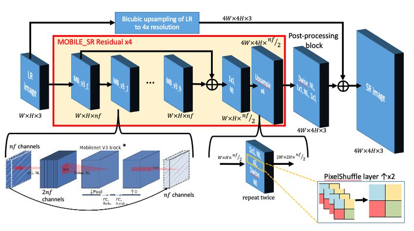
20 K. Zhang et al.

extract different features without significant performance drop, two asymmetric
blocks with inverted kernel order is utilized. Another way to reduce model size
is reducing the scale of feature. Thus an average pooling followed by “Conv-
LeakyReLU-Conv” is utilized, and sub-pixel convolution is used to reconstruct
the HR image. Then the proposed HCSRN is constructed based on this hybrid
module with progressive upsampling strategy as shown in Fig. 17.
 Secondly, the over-parameterized HCSRN is used as the baseline model and
channel pruning is applied to it to further reduce model size. The pruning cri-
terion in [56] is utilized. Instead of employing the group pruning strategy [7,26],
the gating function is asserted before and after each convolution. Thus each
channel is allowed to be pruned independently. To avoid the misalignment prob-
lem between the convolution and the skip connection, the skip connections will
not be pruned and the residual addition operation should always be kept. The
difference between the proposed fine-grained channel pruning strategy and the
previous grouping method is shown in Fig. 16(b). Finally, a pruned lightweight
model called adaptive hybrid composition based super-resolution network (AHC-
SRN) is obtained.

 (a) (b)

Fig. 16. SC-CVLAB Team: (a) the architecture of hybrid composition; (b) an illustra-
tion of baseline structure, structure pruned by group strategy, and structure pruned
by the proposed fine-grained strategy.

HiImageTeam
The HiImageTeam team proposed Efficient SR-Net (ESR-Net) for the chal-
lenge. As shown in Fig. 18(a), ESR-Net achieves an upscaling factor of 4 via
two successive ×2 subnetworks (ESRB). In order to improve the performance,
residual dense network shown in Fig. 18(b) is adopted. L1 loss is used to train
ESR-Net.

SAMSUNG TOR AIC
The SAMSUNG TOR AIC team proposed SAM SR LITE, a Lightweight Mo-
bileNetV3 network for Efficient Super-Resolution [48]. The core of this approach

AIM 2020 Challenge on Efficient Super-Resolution 21

 Fig. 17. SC-CVLAB Team: the network architecture.

 (a) (b)

Fig. 18. HiImageTeam Team: (a) the network architecture; (b) the ESR Block and
Residual Block.

is to use modified MobileNetV3 [16] blocks to design an efficient method for SR.
The authors found that for the MobileNetV3 architecture batch normalization
layers improved the performance. The architecture takes the LR images as in-
put and consists of N+1 modified MobileNetV3 blocks, with a skip connection
(addition) from the output of the first block to the output of the last block.
The output of the last block is then upscaled using the two PixelShuffle opera-
tions [43] with non-linearities and convolutions. To yield three color channels, a
post-processing block containing a depthwise separable convolution and a 1 × 1
convolution layer is applied to the output of the upscaled result. Finally, there is
an additional skip connection between the bicubic upsampling of the LR input
and the output of the post processing block. Fig. 19 provides a overview of the
architecture.
 The hyperparameters include the number of blocks N , the number of feature
mapss nf in each block, and the expansion factor in each block. For the final
submission, N = 16, nf = 72, and the block expansion factor is 2.

neptuneai

The model is based on the MSRResNet and the basic blocks in MSRResNet
is changed to Inverted Residuals Block in MobileNetV2. This architecture is
used as backbone network. Then NAS is used to discover the best architecture
for lightweight SR tasks. A search space which is composed of several kinds of
blocks is designed. The basic blocks for NAS include

22 K. Zhang et al.

 Fig. 19. SAMSUNG TOR AIC Team: the network architecture.

 1. Inverted Residuals Block with 3 expand ration,
 2. Inverted Residuals Block with 6 expand ration,
 3. Basic Residual Block,
 4. Basic Residual Block with leaky ReLU activation function.

lyl

The lyl team proposed Coarse to Fine network (CFN) progressive super-
resolution reconstruction, which contains a CoarseNet and a FineNet. The FineNet
contains a lightweight upsampling module (LUM). There are two characteristics
in CFN, i.e., the progressiveness and the merging of the output of the LUM to
correct the input in each level. Such progressive cause-and-effect process helps
to achieve the principle for image SR. That is, high-level information can guide
an LR image to recover a better SR image. In the proposed network, there are
three indispensable parts: 1) tying the loss at each level, 2) using LUM and
3) providing feature maps extracted in lower level to ensure the availability of
low-level information.

CET CVLab

The architecture used is inspired by wide activation based network and chan-
nel attention network. The network, as shown in Fig. 20, mainly consists of 3
blocks, a feature extraction block, a series of wide activation residual blocks and
a set of progressive upsampling blocks (×2). The expansion factor used for wide
activation block is six. The depth within the feature extraction blocks and wide
activation blocks is 32. The network contains 1.378 million trainable parame-
ters. Charbonnier loss is used for training the network as it captures the edge
information better than the mean squared error (MSE) loss.

AIM 2020 Challenge on Efficient Super-Resolution 23

 Fig. 20. CET CVLab Team: the network architecture.

InnoPeak SR

The InnoPeak SR team proposed Shuffled Recursive Residual Network (SRRN)
for Efficient Image Super-Resolution. As shown in Fig. 21, the proposed SRRN
mainly consists of four parts: shallow feature extraction, residual block feature
extraction, skip connection module, and upscale reconstruction module. To ex-
tract the shallow features, one 3 × 3 convolution layer (pad 1, stride 1, and
channel 64) is used, which is followed by one Leaky ReLU layer (slop 0.1). To
extract the mid-level and high-level features, 16 weights shared recursive resid-
ual blocks are used. The residual block consists of two 3 × 3 convolution layer
(pad 1, stride 1, and channel 64). Only the first convolution layer is followed by
a Leaky ReLU layer (slop 0.1). Batch Normalization (BN) layers are not used.
In this work, one 3 × 3 convolution layer (pad 1, stride 1, and channel 64) and
one sub-pixel convolution layer is used as upscaling module and reconstruction
module. During the training, HR patches of size 196 × 196 are randomly cropped
from HR images, and the mini-batch size is set to 25. The proposed model is
trained by minimizing L1 loss function with Adam optimizer.

Fig. 21. InnoPeak SR Team: an illustration of the proposed SRRN. SRRN consists of
16 residual blocks, but only have four different weights. The residual blocks with same
color share the same parameter weights.

24 K. Zhang et al.

Summer

The Summer team proposed AMAF-Net. The model consists of four parts:
1) Attentive Auxiliary Feature Block (AAF Block) reuses all features of the
preceding blocks as the input feature map of the current layer. By applying
convolution to the concatenated feature maps, the network learns how to com-
bine the information from different blocks. 2) Global residual connection. The
input image are directly upsampled by PixelShuffler, which can be regarded as
a part of the output image. It brings the most basic information to the output.
3) Multi-gradients skip connection. The outputs of each block are upsampled
by 1 × 1 convolution and PixelShuffler. The results are also a proportion of the
output, which are useful for transmitting different frequency information. Mean-
while, gradients can be propagated from the tail of the network to the head.
4) By using the adaptive weight factor multiple outputs are combined with the
learnable parameters, which can adaptively determine the contributions of each
blocks. The network architecture is shown in Fig. 22.
 L1 loss is used in the training process. To further reduce parameters and
FLOPs, the convolution of last two blocks is replaced by 1 × 1 convolution.

 Overall Architecture Global
 Skip

 ILR
 Xskip
 I SR
 Head module Nonlinear Tail module
 mapping

 Xtail

 X0
 X1 X2 X3 X4
 Multi-gradients
 output

 X0
 X1 . . .
 aux
 Xi-1 λ Additive
 Convolution Pixelshuffle Concat Operation
 res Adaptive weight
 λ Xi factor
 Xi-1 (learnable)
 λx ReLU Sigmoid Attentive Auxiliary Multiply
 Feature Block Operation
 Attentive Auxiliary Feature Block

 Fig. 22. Summer Team: the network architecture.

Zhang9678

The Zhang9678 team proposed LFN which contains three parts, including shal-
low feature extraction, deep feature fusion and upsampling. Shallow feature ex-
traction contains a convolutional layer, which is used to map images from image
space to feature space. Deep feature fusion contains four DB blocks and one

AIM 2020 Challenge on Efficient Super-Resolution 25

modified convLSTM. The feature map obtained by the shallow feature extrac-
tion of the image passes through four consecutive DB modules to obtain feature
maps in different depths. LSTM is usually used to process time series data. For
time series data, there is a high degree of similarity between the time steps,
showing a progressive relationship on the time dimension. The feature maps at
different levels are regarded as a kind of pseudo-time series data because they
also contain a progressive relationship at different levels and their similarity is
also high. Specifically, the hidden state h and cell state c of the initial LSTM are
initialized to 0. For each state update, a feature map is selected and sent to the
LSTM along with the corresponding h and c. After the operations in the LSTM,
the new h and c are obtained. This cycle is repeated for four times in total. The
resulting h is concatenated with the shallow features. Then a 1 × 1 convolution
and a 3 × 3 convolution are appended to get the feature map with 48 channels.
Finally, a PixelShuffler is used to get the final SR image.

 Fig. 23. Zhang9678 Team: the network architecture.

H-ZnCa
The H-ZnCa team proposed Sparse Prior-based Network for Efficient
Image Super-Resolution. As shown in Fig. 24(a), the proposed lightweight
model, named SPSR, consists of three components: high-frequency sparse coding
generation, feature embedding, and multi-scale feature extraction. Specifically, a
convolutional sparse coding module (CSCM) [45,29] is first performed to obtain
the high-frequency spare representation of the input. Then, a feature embedding
block (FEB) [49] which consists of a Spatial Feature Transform (SFT) layer and
two convolutional layers is designed for spatial-wise feature modulation condi-
tioned on the sparse prior representation. To further enhance the abstract ability
of SPSR, a multi-scale feature extraction module (MFEM) with channel split
mechanism is proposed to efficiently utilize the hierarchical features. As shown in
Fig. 24(b), MFEM contains several convolutions with different dilation factors.

26 K. Zhang et al.

 Bilinear Input tensor
 (c, h, w)

 Feature Embedding Block Feature Embedding Block Conv 1x1

 Feature Extraction
 Input tensor
 Intermediate tensor Intermediate tensor
 (c, h, w)

 Leaky ReLU
 Instance Norm

 Leaky ReLU

 Instance Norm
 (c/2, h, w) (c/2, h, w)

 Multi-scale

 Upsampling
 Conv Layer

 Conv Layer

 Conv Layer

 Conv Layer

 Conv Layer
 SFT Layer

 SFT Layer
 Conv 3x3 Conv 3x3 Conv 3x3
 ... Rate=2 Rate=2
 Intermediate tensor Intermediate tensor Intermediate tensor Intermediate tensor
 (c/4, h, w) (c/4, h, w) (c/4, h, w) (c/4, h, w)

 Detail Features Conv 3x3 Conv 3x3 Conv 3x3 Conv 3x3
 Rate=3 Rate=5 Rate=3 Rate=5
 Conv Ɗ

 Element-wise Sub
 Concat
 Conv Ǫ

 Conv Ǫ
 Conv Ɍ

 Conv Ɍ
 S S S Soft Threshold
 Output tensor
 Convolutional Sparse Coding Conv 1x1 (c, h, w)

 (a) (b)

Fig. 24. H-ZnCa Team: (a) the architecture of SPSR Network; (b) the multi-scale
feature extraction module (MFEM).

MLP SR

The MLP SR team proposed a lightweight deep iterative SR learning method
(ISRResDNet) that solves the SR task as a sub-solver of image denoising by the
residual denoiser networks [24]. It is inspired by powerful image regularization
and large-scale optimization techniques used to solve general inverse problems.
The proposed iterative SR approach is shown in Fig. 25. The authors unroll the
ResDNet [24] into K stages and each stage performs the PGM updates.

Fig. 25. MLP SR Team: the architecture of the iterative SR approach ISRResDNet.

Acknowledgements

We thank the AIM 2020 sponsors: HUAWEI, MediaTek, Google, NVIDIA, Qual-
comm, and Computer Vision Lab (CVL) ETH Zurich.

A Teams and affiliations

AIM2020 team

Title: AIM 2020 Efficient Super-Resolution Challenge
Members:
Kai Zhang (kai.zhang@vision.ee.ethz.ch),
Martin Danelljan (martin.danelljan@vision.ee.ethz.ch),

AIM 2020 Challenge on Efficient Super-Resolution 27

Yawei Li (yawei.li@vision.ee.ethz.ch),
Radu Timofte (radu.timofte@vision.ee.ethz.ch)
Affiliations:
Computer Vision Lab, ETH Zurich, Switzerland

NJU MCG
Title: Residual Feature Distillation Network (RFDN)
Members: Jie Liu
(jieliu@smail.nju.edu.cn), Jie Tang, Gangshan Wu
Affiliation:
State Key Laboratory for Novel Software Technology, Nanjing University, Nan-
jing 210023, China

AiRiA CG
Title: Faster Information Multi-distillation Network via Asymmetric Convolu-
tion
Members: Yu Zhu
(zhuyu.cv@gmail.com), Xiangyu He, Wenjie Xu, Chenghua Li, Cong Leng, Jian
Cheng
Affiliation:
Nanjing Artificial Intelligence Chip Research, Institute of Automation, Chinese
Academy of Sciences (AiRiA); MAICRO

UESTC-MediaLab
Title: Efficient Super-Resolution with Gradually Kernel Dilution
Members: Guangyang Wu1
(mulns@outlook.com), Wenyi Wang1 , Xiaohong Liu2
Affiliation:
1
 University of Electronic Science and Technology of China
2
 McMaster University

XPixel
Title: Efficient Image Super-Resolution using Pixel Attention
Members: Hengyuan Zhao
(hy.zhao1@siat.ac.cn), Xiangtao Kong, Jingwen He,Yu Qiao, Chao Dong
Affiliation:
Shenzhen Institutes of Advanced Technology, Chinese Academy of Sciences

28 K. Zhang et al.

HaiYun
Title: Lightweight Image Super-resolution with Lattice Block
Members: Xiaotong Luo
(xiaotluo@qq.com), Liang Chen, Jiangtao Zhang
Affiliation:
Xiamen University, China

IPCV IITM
Title: Lightweight Attentive Residual Network for Image Super-Resolution
Members: Maitreya Suin
(maitreyasuin21@gmail.com), Kuldeep Purohit, A. N. Rajagopalan
Affiliation:
Indian Institute of Technology Madras, India

404NotFound
Title: GCSR
Members: Xiaochuan Li (1182784700@qq.com)
Affiliation:
Nanjing University of Aeronautics and Astronautics, Nanjing, China

MDISL-lab
Title: PFSNet: Partial Features Sharing for More Efficient Super-Resolution
Members: Zhiqiang Lang
(2015303107lang@mail.nwpu.edu.cn), Jiangtao Nie, Wei Wei, Lei Zhang
Affiliation:
School of Computer Science, Northwestern Polytechnical University, China

MLVC
Title: Multi Attention Feature Fusion Super-Resolution Network
Members: Abdul Muqeet1
(amuqeet@khu.ac.kr), Jiwon Hwang1 , Subin Yang1 , JungHeum Kang1 , Sungho
Bae1 , Yongwoo Kim2
Affiliation:
1
 Kyung Hee University, Republic of Korea
2
 Sang Myung University, Republic of Korea