From Patch to Image Segmentation using Fully Convolutional Networks - Application to Retinal Images - arXiv
←
→
Page content transcription
If your browser does not render page correctly, please read the page content below
From Patch to Image Segmentation using Fully
                                        Convolutional Networks - Application to Retinal Images
                                          Taibou Birgui Sekoua,b,c,d , Moncef Hidanea,b,c , Julien Oliviera,b,c , Hubert
                                                                          Cardotb,a,c
arXiv:1904.03892v1 [cs.CV] 8 Apr 2019

                                             a
                                                 Institut National des Sciences Appliquées Centre Val de Loire, Blois France
                                                                     b
                                                                       Université de Tours, Tours, France
                                                                       c
                                                                         LIFAT EA 6300, Tours, France
                                                           d
                                                             Corresponding author: taibou.birgui sekou@insa-cvl.fr

                                        Abstract
                                        In general, deep learning based models require a tremendous amount of sam-
                                        ples for appropriate training, which is difficult to satisfy in the medical field.
                                        This issue can usually be avoided with a proper initialization of the weights.
                                        On the task of medical image segmentation in general, two techniques are
                                        usually employed to tackle the training of a deep network fT . The first one
                                        consists in reusing some weights of a network fS pre-trained on a large scale
                                        database (e.g. ImageNet). This procedure, also known as transfer learn-
                                        ing, happens to reduce the flexibility when it comes to new network design
                                        since fT is constrained to match some parts of fS . The second commonly
                                        used technique consists in working on image patches to benefit from the large
                                        number of available patches. This paper brings together these two techniques
                                        and propose to train arbitrarily designed networks, with a focus on relatively
                                        small databases, in two stages: patch pre-training and full sized image fine-
                                        tuning. An experimental work have been carried out on the tasks of retinal
                                        blood vessel segmentation and the optic disc one, using four publicly avail-
                                        able databases. Furthermore, three types of network are considered, going
                                        from a very light weighted network to a densely connected one. The final
                                        results show the efficiency of the proposed framework along with state of
                                        the art results on all the databases. The source code of the experiments is
                                        publicly available at https://github.com/Taib/patch2image.
                                        Keywords: Retinal image segmentation, Transfer learning, Deep learning

                                        Preprint submitted to Medical Image Analysis                                 April 9, 2019
1. Introduction
    The task of image segmentation consists in partitioning an input picture
into non-overlapping regions. On medical images, it aims at highlighting
some regions of interest (ROIs) for a more in-depth study/analysis. The
result of a segmentation can then be used to extract various morphological
parameters of the ROIs that bring more insights into the diagnosis or control
of diseases. On a retinal image, the ROIs include the blood vessels and the
optic disc (the optic nerve head), as depicted in Figure 1. Retinal blood
vessel segmentation (RBVS) is helpful in the diagnosis, treatment and moni-
toring of diseases such as the diabetic retinopathy, the hypertension and the
arteriosclerosis [1, 2]. Optic disc segmentation (ODS) can bring relevant in-
sights on the glaucoma disease [1]. Nowadays, these diseases are the leading
factors of blindness [3, 4].
The manual annotation of the blood vessels (or the optic disc) is an ar-
duous and time consuming work that requires barely-accessible expertise.
Moreover, not only do expert segmentations are subject to inter- and intra-
operator variability, they also become impractical for large-scale and real-
time uses. Hence the large amount of work in designing automatic methods
[5, 6]. In the following, retinal image segmentation (RIS) refers to either
blood vessel or optic disc segmentation.
    More generally, medical image segmentation has undergone tremendous
advances which are mainly due to deep convolutional neural networks (DC-
NNs). A DCNN is a mathematical model that applies a series of feature
extraction operators (a.k.a. the convolution filters) on the input to obtain a
high level abstract representation. The latter can then be used as input to
a classifier/regressor [7]. The model can be trained in a supervised manner
using a training set. When employing DCNNs, image segmentation can be
cast as a classification task where the goal is to label each pixel of the input
image.
    On the task of RIS, the DCNN-based propositions can be grouped by
their type of input/output: patch-to-label, patch-to-patch, and image-to-
image. The last two groups are also known as end-to-end approaches and
are usually based on particular DCNN architectures: the fully convolutional
neural networks (FCNNs) [8].
    The patch-to-label group trains a network that takes an image patch
(small window inside the image) as input and produces the label of its center
pixel. A natural variation consists in assigning labels to a subset of the

                                       2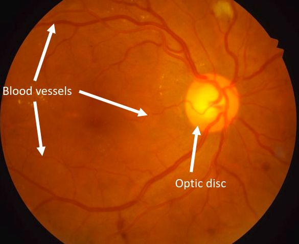
Figure 1: Illustration of a retinal image and some structures therein. (For interpretation
of the references to color in this figure legend, the reader is referred to the web version of
this article.)

input patch. Then, given a test image, one classifies each pixel using a
surrounding patch. Thus, the segmentation can be cast as an independent
patch classification task. Besides being time consuming, these approaches
usually fail when the objects are on the frontiers of two classes. This is mainly
due to the loss of contextual/structural information in the final layers.
    These drawbacks can be alleviated by using a patch-to-patch network.
It consists in using a network that can output a segmentation map for each
given patch. In other words, the network labels each pixel of the patch. As
a consequence the segmentation task is performed in three stages: a patch
extraction from the input image followed by a pass through the network to
obtain the segmentation maps, finally these maps are aggregated to output
the final segmented image. These approaches reduce the previous frontiers’
objects issue though the patch aggregation stage may still be time consuming
especially for real-time applications.
    Note that the patch-based methods require a certain level of discrimina-
tive information in the patches, for them to be efficient. When this require-
ment is hard to fulfill (e.g. the ROIs occupy the quasi-totality of the image),
it might be beneficial to work directly on the full-sized images. The image-
to-image networks take the entire image as input and produce the complete
segmentation in one forward pass through the network. They have the ad-

                                              3
vantage of being well adapted for real-time applications and can be seen as
a generalization of the patch-to-patch approach with a large patch size.
Regarding the training of DCNNs, an important effort needs to be ded-
icated to building the corresponding training sets. In general, a well built
training set satisfies the following: (i) it contains different examples of each
sought invariance, and (ii) it consists of a large number of samples. Un-
fortunately, these requirements are often hard to meet in the medical field:
medical images are hard to obtain and very difficult to annotate. Neverthe-
less, DCNN-based models have been successfully applied in the medical field
[9, 10], in particular on the task of RIS [5, 6].
The first trick used in training DCNNs for RIS is to work at the patch
level (i.e. using either a patch-to-label approach or a patch-to-patch one). Al-
lowing for patch overlap when extracting training patches leads to large-scale
training sets, thus facilitating the training of arbitrarily designed networks
[11, 12].
When working at the image level (i.e. using an image-to-image approach)
two tricks are usually combined to train DCNNs on small sized databases.
The first one, known as data augmentation, consists in adding to the ini-
tial database scaled and rotated versions of the training samples. It helps
boosting the training set and to some extent avoiding over-fitting. Yet, the
training set may still be very small compared to the number of parameters
in the model. The second technique, known as transfer learning, consists in
reusing the parameters of a network fS trained on a source database DS to
improve the performance of a network fT to be learned on a target database
DT , as depicted in Figure 3. Consequently, the architecture of the network
fT is somehow predefined by the one of fS since, for fT to reuse some weights
of fS , the architecture of the two networks must match at least at the shared
weights locations. Transfer learning aims at finding a good starting point
for the weights and helps training very deep networks on relatively small
datasets [13, 14].
Generally, on the task of RIS, the proposed networks so far are either
trained at the patch level or at the image level. Those that are trained
at the patch level can benefit from a freely designed architecture, whereas
those that are trained at the image level should conform to previously de-
fined architectures (usually the VGG of [15]). This paper presents a training
framework that bridges the gap between the two levels and provides a way
to have freely designed networks working efficiently both at the patch- and
image-levels even on small sized databases. The liberty in the network design
4opens up the door for more research on deep architectures for RIS, with the
hope of reaching findings as remarkable as those obtained for natural images
such as AlexNet [16], VGG [15], ResNet [17] and DenseNet [18]. It also pro-
vides a way to build budget-aware architectures [19, 20] that can suit different
clinical constraints (e.g. lightweight networks for embedded systems).
How to obtain state-of-the-art performances using a freely designed image-
to-image network on the task of RIS? If the size of the database at hand
is consequent then the challenge is in building an appropriate network and
pre-processing the data. This case has been well studied in the natural im-
age literature. However, for small sized database, generally encountered in
the medical field (especially on RIS tasks), existing works are generally not
freely designed image-to-image models. The focus on freely designed image-
to-image models leads to fast and easy to use domain specific architectures.
Thus, in this paper the small sized database case is elaborated. The follow-
ings are presented:
• The proposed framework consists of four phases. The first two take ad-
vantage of the large-scale training samples available at the patch level
to train the networks from scratch (i.e. from random initialization).
The last two phases consist of a transfer learning from the patch net-
works weights to the image ones and a fine-tuning to adapt to weights
and improve the segmentation.
• To assess the results of the proposed framework, 3 types of network are
considered. The networks vary in terms of architectural complexity and
number of weights: (1) a lightweight network (Light) of 8, 889 weights,
(2) a reduced UNet-like [21] network (Mini-Unet) of 316, 657 weights,
and (3) a deep densely connected one (Dense) of 1, 032, 588 parameters
inspired from [18].
• Concerning the databases, the experiments have been carried out on
four publicly available databases with a relatively small number of
training samples. On the task of RBVS, three databases are used for
evaluation: DRIVE, STARE, and CHASE DB1. Whereas the IDRID
is used for the ODS task.
• The quantitative results show state-of-the-art results of the final image-
to-image networks. Furthermore, they prove that all the patch-based
networks can be extended to work directly at the image level with a
5performance improvement. All the phases of the proposed framework
are analysed to point out their importance. On the other hand, using
the framework, we show that on some databases the Light network
can perform as good as other complex state-of-the-art networks while
staying by far more simple and segmenting an entire image in one
forward pass.
The rest of the paper is organized as follows. Sec. 2 gives an overview
of the related work. After a brief introduction to DCNNs (Sec. 3) and
transfer learning (Sec. 4), Sec. 5 presents the proposed framework. Sec. 6
presents the experimental work including the used DCNNs, the databases
and their associated pre-processing along with the results and discussions.
We summarize the proposed work in Sec. 7 and provide some perspectives.
2. Related Work
In the following, some recent deep learning based propositions on RIS are
listed and grouped by their training strategy: patch- and image-based. For
a more detailed review see [5, 6, 22].
2.1. Patch-based training
On the task of RBVS, Liskowski and Krawiec [11] proposed a freely de-
signed patch-to-label DCNN which is further extended to output a small
patch centered on the input. The network is trained from scratch using
27 × 27 RGB patches. In [23], an additional complexity constraint is im-
posed on the patch-to-patch network. The goal was to build networks that
work efficiently on real-time embedded systems, for example a binocular in-
direct ophthalmoscope. Oliveira et al. [24] proposed a patch-to-patch model
and added a stationary wavelet transform pre-processing step to improve
the network’s performance. On the other hand, [25] chose to use plain RGB
patches but reused the AlexNet network [16] which is pre-trained on the Ima-
geNet dataset. Other propositions include [26, 27, 12], where freely designed
patch-to-patch networks are once again trained from scratch.
On the task of optic disc segmentation, Fu et al. [28] presented a multi-
level FCNN with a patch-to-patch scheme which aggregates segmentations
from different scales. The network is applied on patches centered on the optic
disc. Therefore, an optic disc detection is required beforehand. Tan et al.
[29] proposed a patch-to-label network which classifies the central pixel of an
6input patch into four classes: blood vessel, optic disc, fovea, and background.
Because of the lack of training data, most of the RIS models are patch-based.
However, some propositions have been made using an image-to-image scheme
based on weights transfer from the VGG network.
2.2. Image-based training
In a more general setting of medical image segmentation, Tajbakhsh et al.
[13] showed experimentally that training with transfer learning performs at
least as good as training from scratch. On the task of RBVS, Fu et al. [30]
used the image-to-image HED network [31] and added a conditional random
field post-processing step. They performed a fine-tuning from the HED which
is based on the VGG of Simonyan and Zisserman [32]. Mo and Zhang [33]
proposed to reuse the VGG and added supervision at various internal layers
to prevent the gradient from vanishing in the shallower layers. A similar
technique has been used by Maninis et al. [34] with an additional path to
segment both the blood vessels and the optic disc.
2.3. From patch- to image-based training
A proof of concept is presented in our previous work [35]. Promising
results have been obtained when using the patch network’s weights as an ini-
tialization point of the image network. However the patch network’s metrics
tend to be better than the image ones. This remark may question the im-
portance of the transfer. Moreover, only one database and a single network
have been considered. Hence, one may question the generalization to other
databases and networks.
This paper redefines the framework in a more detailed manner and applies
it to three types of networks. The networks are trained with a segmentation-
aware loss function using decay on the learning rate to avoid the over-fitting
observed in the previous work when fine-tuning at the image-level. Fur-
thermore, the experiments have been carried out on four publicly available
databases. The final results prove that the results of the patch network can
be improved using the framework.
3. Convolutional Neural Networks
With a first success in the late 80’s [36], DCNNs are nowadays the method
of choice in diverse areas, particularly in computer vision including image
classification [17, 18, 32], image segmentation [8], image generation [37], to
7Figure 2: A toy example FCNN. The input and output are of size 4 × 4. The highlighted
blue cells represents the zero-padding applied before each convolution to maintain the
input size. The convolution kernels are given on top of the black arrows. The red arrow
corresponds to the point-wise rectified linear unit function: x 7→ max(x, 0). The gray
arrow applies a max-pooling in 2 × 2 windows with a stride of 2. The orange arrow is an
up-sampling layer that duplicate the values in a 2 × 2 window. The green arrow consists
in applying the sigmoid function, point-wise. (For interpretation of the references to color
in this figure legend, the reader is referred to the web version of this article.)
name a few. As stated in the introduction, DCNNs for classification con-
sist in extracting highly abstract and hierarchical representations from the
data that are fed into a classifier/regressor. They consist of different types
of layers that are stacked on top of each other to form the final model.
Commonly used layers include: the convolution layer, non-linearity (ReLU,
Sigmoid, ELU), normalization (batch-normalization), pooling (max-pooling,
average-pooling), dropout, fully connected, etc. The convolution and fully
connected layers aim at learning high-level patterns from the database that
can improve the representation. On the other hand, pooling, non linearity
and normalization layers aim at adding more invariance into the representa-
tion and ameliorating the generalization power. A clear view of these models
can be found in [38, 39, 40].
On the task of image segmentation, state-of-the-art DCNN-based mod-
els are usually fully convolutional neural networks (FCNNs). FCNNs are a
variation of DCNNs that do not include fully connected layers [8]. Hence,
they allow the spatial/structural information of the input to be preserved
across the network. As a consequence, one can build end-to-end like net-
works where the output and the input are of the same shape. Therefore
one can directly train a network to segment an entire image in one forward
pass. Additional layers that appear in FCNNs, used to recover the size of
the input, are the transposed convolution (a.k.a deconvolution) layer and
the up-sampling (a.k.a duplication) one. Another advantage of the FCNNs,
8Figure 3: Classical transfer learning. Step 1: Train the network fS on a large scale database
(e.g. ImageNet). Step 2: Build a task specific network fT that reuse some weights of fS .
Step 3: Fine-tune the network fT on DT .
inherited from the convolutions, is the input size invariance. That is, a same
FCNN can be applied to inputs of various size as long as they all share the
same number of spatial dimensions and channels. For example, the FCNN
of Figure 2 can, as well, take inputs of shape 400 × 400 to output a 400 × 400
image.
Hereafter, a convolutional network h is characterized by its associated set
of parameters θ. Typically, if h is FCNN then θ will be of the following form:
θ = {{Wl,k , bl,k }K L
k=1 , σl }l=1 ,
l
(1)
where L is the number of layers, Kl is the number of kernels in the l-th layer,
σl is the l-th activation function, Wl,k is the k-th kernel (the convolution
kernel) of the layer k, and bl,k is the associated bias.
4. Transfer Learning
In the case of DCNNs, transfer learning consists in reusing the “knowl-
edge” learned by a network NS trained on a source database DS to ameliorate
the performance of a network NT on a target database DT , with DS 6= DT
(see Figure 3). Here a database Di consists of two elements: the input data
Xi and their targets Yi . Thus DS 6= DT means (1) XS 6= XT and/or (2)
YS 6= YT . In other words, either (1) the inputs are different (e.g. natural im-
ages v.s. medical images, patches v.s. images) or (2) the targets are different
(e.g. retinal blood vessels v.s. optic discs).
The knowledge in a DCNN lies in its weights (i.e. the convolution filters)
learned throughout the training. DCNNs based transfer learning can be seen
9as a feature-representation-transfer and a hyper-parameter-transfer. It is a
hyper-parameter-transfer since transferring some knowledge from Ns to Nt
implies the reuse of part of the architecture of fS in fT . The architecture per
se of a DCNN is a hyper-parameter. Concerning the feature-representation-
transfer, the transferred weights will write inputs from DS and DT in the same
feature space. Therefore, the weights’ transfer constrains the two networks
to share the same feature representation.
There are mainly three major concerns when transferring knowledge of
DCNNs: what to transfer, when to do it, and how to perform it [41]. An-
swering these questions helps avoiding a negative transfer, that is, degrading
the performance on the target database.
What to transfer is equivalent to knowing which weights to transfer. In other
words, which part of the architecture of fS will be reused in fT . While the
weights in the first layers of a DCNN capture abstract patterns of the data,
the ones in the deeper layers (especially the last layer) are more task specific.
The work of Yosinski et al. [14] provides a more detailed experimental work
on how much abstracted are the learned weights.
The when to transfer question asks which couple (DS , fS ) is well suited to
transfer from. For example, the current state-of-the-art results on transfer
learning advise to have at least two databases of the same types (i.e. image
to image, audio to audio).
The last question (how to transfer) is resolved mainly with a copy-paste of
the weights from one network to another. Then, one can either keep the
transferred weights frozen or fine-tune them. If frozen, the weights are not
updated, while, the fine-tuning case continues to update the weights using
the target database. In the latter case, transfer learning is equivalent to
weight initialization.
Most DCNNs based RIS systems that perform transfer learning reuse the
convolution layers of the VGG network and add some additional task specific
layers. As a consequence, the final network’s architecture is no longer freely
designed. Often, RIS may not need an extremely sophisticated network to
achieve good results. In the following, a proposed framework to train a freely
designed network on RIS tasks is presented.
5. The Framework
Given a database DI of retinal images (and their corresponding annota-
tions) our principal task is to freely design and train a FCNN efficiently. As
10Figure 4: Flowchart of the proposed framework. DI is the database of the original full-
sized images. Patches are extracted from the images of DI to build DP . fP is the network
trained on DP , while fI is the one trained on DI . (For interpretation of the references to
color in this figure legend, the reader is referred to the web version of this article.)
aforementioned, for the considered RIS databases and the medical field in
general, DI usually is of relatively small size which makes difficult the train-
ing of complex FCNNs architecture. This issue is commonly addressed by
working at the patch level [42]. Therefore, the proposed framework makes
use of the patch level information to build large-scale patch database. Fig-
ure 4 depicts the four main components of the framework which are detailed
in the following. Before detailing the components, we start by given some
theoretical motivation of the framework.
5.1. Theoretical Motivation
For the sake of notation simplicity, we consider a binary image seg-
mentation task with square-shaped images with one channel. Namely, let
I ⊂ Md (R) be the d2 -dimensional image space and S ⊂ Md ({0, 1}) be the
associated segmentation space such that there exists an oracle f : I → S that
assigns to each image X ∈ I its unique segmentation Y = f (X). Suppose
the images are sampled from a distribution Px , whose support is precisely
the set I. The objective is to approximate
h f with a parametrized
i function f˜
that minimizes the expected loss EX∼Px r(f˜(X), f (X)) , where r is a certain
11elementary loss function. In practice, the expectation is approximated by the
empirical mean over a dataset D = {Xi , Yi = f (Xi )}ni=1 of n samples with
Xi ∈ I and Yi ∈ S. In other words, f˜ is given by
n
X
f˜ = arg min (1/n) r(h(Xi ), f (Xi )), (2)
h∈H i=1
where H is the class of parametrized functions in use. In our case, H is
the set of functions that correspond to a forward pass through our neural
network. On the task of RIS, one might want to start the segmentation
locally (in smaller neighborhoods) then fine-tune it by looking at the entire
image. Using this idea, the optimization problem of Eq. 2 involving d2 -
dimensional I images now involves p2 -dimensional patches, where p is the
size of neighborhoods. This introduces the use of patch-based approaches
that are discussed in the following.
An image X ∈ I can be written as a combination of p2 -dimensional
patches by constructing a set of functions {νk , εk }Pk=1 , with P the number of
patches, such that:
XP
X= νk (εk (X)), (3)
k=1
where, for all k, εk : I → Mp (R), and νk : Mp (R) → I. The function εk
extracts the kth patch while νk plugs the latter in the image and handles
the possible overlap. In Eq. 3, we are assuming that each pixel of X can
be reconstructed from the patches it belongs to. For instance, if we consider
non-overlapping patches of M2 (R) and d = 6 then
2 X
X 2
X= ATr Ar XATs As ,
r=0 s=0
2
where Ak = Ak−1 J0,6 ∈ M2,6 ({0, 1}) for all k ≥ 1, J0,6 is the 6 × 6 Jordan
matrix with 0 as eigenvalue and
1 0 0 0 0 0
A0 = ∈ M2,6 ({0, 1}).
0 1 0 0 0 0
So for a fixed r and s, the matrix Ar XATs is an element of M2 (R). It is
worth noting that, patch-based approaches are only applicable on separable
segmentation tasks.
12Definition (Separability). Using the previous notation, a segmentation task
associated to f is said to be separable if there exists a family of functions
{gk : Mp (R) → Mp ({0, 1})}Pk=1 such that
P
X
f (X) = νk (gk (εk (X))), for all X ∈ I. (4)
k=1
In particular, the separation is said to be simple –which we will assume in the
sequel– when gk = g for all k. In other words, by assuming the separability
condition, one hypothesizes that the patches extracted by εk contain enough
information to classify each element therein. With this condition, the d2 -
dimensional problem of segmenting an image is now broken down into a
series p2 -dimensional one. However, as aforementioned, the drawbacks of the
patch-based works include:
- The time complexity: If we assume the patch extractors and mergers
(i.e. the εk ’s and νk ’s) to have a O(1) complexity then the overall
segmentation will be in O(P Cg ) where Cg is the time complexity of the
patch model g and P is the number of patches. The commonly used
trick parallelizes the procedure and is still time consuming for large
values of P , as shown in our experiments.
- The overall segmentation homogeneity: On the other hand, in practice,
the separability assumption leads to a lack of overall segmentation ho-
mogeneity. That is, the patch model g of Eq. 4 is restricted on a small
neighborhood and may fail for some objects where a larger neighbor-
hood is required for better results. Thus the need to an additional
post-processing step in many patch-based.
- Breaking the posterior distribution: Given an input patch x and its
associated true segmentation s, the patch network g approximate the
conditional distribution P(s|x). However, after a standard patch ag-
gregation procedure, the final segmentation is no longer following g’s
distribution. This problem has been clearly discussed in the context of
inverse imaging problems in Zoran and Weiss [43]. Therefore, it might
be beneficial to learn complex aggregation models.
In this paper, the function f is approximated by a FCNN function f˜,
characterized by θ, the set of weights and biases of Eq. 1. Our framework
13aims at avoiding any aggregation step and ensures an overall segmentation
homogeneity. To do so, we start by assuming the simple separability as-
sumption of Eq. 4 to train a patch network g̃ to obtain a well optimized
set of weights θg . Then, to decrease the running time and improve the over-
all homogeneity, we adapt θg to capture more information about the entire
image, that is the final network f˜ will have as parameters θf , obtained by
fine-tuning θg . The procedures are explained step by step in the sequel and
are depicted in Figure 4.
5.2. The Different Phases in Practice
Each phase depicted in Figure 4 of the proposed framework is explained
in the following.
• Phase 1: Patches are extracted from the training images to build
the patch database. The latter becomes the source database, denoted
DP . Recall that it is not enough to extract a large number of patches.
One should also ensure the diversity of the patches in order to have
in a balanced proportion all the possible cases. The extraction can be
made in a grid manner or randomly.
• Phase 2: A network fP is freely designed and trained, from scratch,
on the previously built patch database DP . With a well constructed
patch database, it becomes easier to train fP from scratch, since DP
provides the major requirements for training: enough training samples
and diversification. Recall that, to segment an original full-sized im-
age with fP a patch extraction step is performed followed by patch
segmentation and finally a patch aggregation step is needed.
• Phase 3: The network fI is built based on the architecture of fP .
The transfer learning occurs here in the framework. In this work, the
transfer consists in copying all the weights of fP into fI . To assign
a label (blood vessels, optic disc) to a pixel, a small neighborhood is
analyzed. The latter can be found both in a patch containing the pixel
and (obviously) in the entire image. Thus, it is natural to infer that
the weights used to segment patches should produce acceptable results
when applied on the original images.
• Phase 4: This final phase aims at adapting the transferred weights
(of fP ) to work properly on DI . These weights, being learned from
14small patches, may not take into account the overall homogeneity of
a full-sized image segmentation. As a consequence, the network fI is
fine-tuned on the full-sized images. In practice, this phase should be
handled with special attention to avoid a negative transfer and/or an
over-fitting.
How general is the framework? Notice that commonly used training pro-
cedures can be cast as special cases of the proposed framework. Literature
training methods can be grouped in two categories (see Section 2): patch-
based, images-based. The patch-based methods are equivalent to using only
the phases 1 and 2 of the framework. Recall that an additional patch ag-
gregation is needed to obtain the final segmentation. By setting the patch
database to be ImageNet and using the VGG network as fP , habitual trans-
fer learning based training propositions can be cast as special case of the
proposed framework.
6. Experiments
This section details all the experimental set-up and the final results, start-
ing with a brief presentation of the databases.
6.1. Databases
The following databases are considered: DRIVE, STARE, CHASE DB1
for the task of RBVS and IDRiD for the ODS one. On the first three the test
images are manually annotated by two human observers, and as practiced in
the literature, we used the first observer as a ground-truth to evaluate our
methods. On all the databases, the images are resized, first, for computa-
tional reasons to avoid memory overload, and because of the networks, since
there is a downsize of factor 4 in the architectures. However, all the seg-
mented images are resized back to their initial size to compute the metrics.
In the following, the initial and resized sizes are given for each database.
DRIVE (Digital Retinal Images for Vessel Extraction) [44]1 is a dataset
of 40 expert annotated color retinal images taken with a fundus camera of
size 584 × 565 × 3. The database is divided into two folds of 20 images:
the training and testing sets. A mask image delineating the field of view
1
http://www.isi.uu.nl/Research/Databases/DRIVE/
15Figure 5: Illustration of the used networks. The layers used in Light and MUnet are
described in between their drawing. The ones in the Dense network are grouped by
block. The dark-blue squares correspond to the densely connected parts and the inscribed
digit within is the number of blocks (an example is given with 2 dense blocks). (For
interpretation of the references to color in this figure legend, the reader is referred to the
web version of this article.)
16(FOV) is provided but not used in our experiments. The images are resized
to 584 × 568 × 3.
STARE (STructured Analysis of the REtina)2 [45] is another well known,
publicly available, database. The dataset is composed of 20 color fundus
photographs captured with a TopCon TRV-50 fundus camera at 35◦ field
of view. Ten images are pathological cases and contain abnormalities that
make the segmentation task even harder. Unlike DRIVE, this dataset does
not come with a train/test split, thus a 5-fold cross-validation is performed.
The images are of size 605 × 700 and resized to 508 × 600 × 3.
CHASE DB13 [46] consists of 28 fundus images of size 960 × 999 × 3.
They are acquired from both the left and right eyes of 14 children. On this
dataset, a 4-fold cross-validation is performed. The images are resized to
460 × 500 × 3.
IDRiD (Indian Diabetic Retinopathy Image Dataset)4 [47] is a publicly
available dataset introduced during a 2018 ISBI challenge. It provides expert
annotations of typical diabetic retinopathy lesions and normal retinal struc-
tures. The images were captured with a kowa VX-10 alpha digital fundus
camera. The optic disc segmentation task is considered in this paper. IDRiD
consists of 54 training images of size 2848 × 4288 × 3 and 41 testing ones. In
our experiments, the images are downscaled by 10 to obtain 284 × 428 × 3
size.
Building the patch databases The patches are extracted based on the
distribution of the class labels in the ground-truths. On the task of RBVS,
as illustrated on Fig. 6, the blood vessels are spread across the ground-truth.
As a consequence, the patches are extracted with a stride of 16. While on
IDRiD the optic disc pixels are localized in a small region of the ground-truth
image. Hence, the patch database is built by extracting 500 patches centered
on randomly selected optic disc pixel and another 500 on the background
pixels.
Pre-processing The success of DCNN-based models depends on the
pre-processing performed on the data beforehand. The pre-processing step
aims mainly at improving the quality of the input data. The following pre-
processing is performed on each RGB image of all the databases: (1) gray-
2
http://www.ces.clemson.edu/~ahoover/stare/
3
https://blogs.kingston.ac.uk/retinal/chasedb1/
4
https://idrid.grand-challenge.org/
17Figure 6: Qualitative results using the Dense network on: the 01 DRIVE image, the 0044
STARE image, the 66 IDRiD image, and the 02L CHASE one. From top to bottom: the
original image, the ground-truth, the result after a training from scratch, the patch-based
segmentation, the result a the image level with a frozen transfer, and the result after
fine-tuning. The red arrows show some cases where the probabilities are strengthen after
fine-tuning to obtain solid lines while the yellow ones show an examples of false positives’
removing. (For interpretation of the references to color in this figure legend, the reader is
referred to the web version of this article.)
18scale conversion, (2) a gamma correction (with gamma set to 1.7), and (3) a
Contrast Limited Adaptive Histogram Equalization (CLAHE). The patches
on all databases are extracted after the pre-processing step.
6.2. The Networks
Three networks have been used in this paper: a standard lightweight
FCNN of 8, 889 weights (Light), a reduced version of the U-Net of 316, 657
weights (MUnet), and a densely connected network of 1, 032, 588 parameters
(Dense). All these networks have an end-to-end structure and can thus pro-
cess inputs of arbitrarily sized (i.e. patches or images). The architectural
details are depicted in the figure 5.
The Light network is a simple FCNN with 8 filters on each layer. With
its 8, 889 weights this network is very light and very suitable for low memory
embedded systems. Moreover, it also provides some insights on the complex-
ity of the task at hand. In other words, if the Light network’s performances
are not very far from the other (state-of-the-art) complex networks, then one
can conclude that the task is not very difficult and can be solved with a small
number of parameters.
The MUnet network with 316, 657 trainable parameters is a reduced
version of the U-Net[21]. It is less complex than the Dense network in terms
of architecture and uses a relatively small number of weights in each layer.
The Dense network consists of an overall of 1, 032, 588 trainable param-
eters. It is based on the densely connected design of Huang et al. [18]. In
the dense blocks (dark-blue squares), the output of each intermediate layer
`i is stack channel-wise on top of the one of `i−1 to feed the layer `i+1 . In
this network, three variables (Ω, Π, and ∆) are used to adapt the number of
filters after each layer. Ω is initially set to 8 and increased by 2 after each
concatenation while ∆ = Ω ∗ 4 and Π = Ω ∗ 0.5.
6.3. Training setup
Regarding the training procedure, it has been carried out as described in
the following.
• A combined loss function which is defined, given a ground-truth y ∈
{0, 1}n and a prediction p ∈ [0, 1]n , by
2hy, pi
`(y, p) = −hy, log(p)i − ,
hy, 1i + hp, 1i
19where log(p) = [log(p[1]), ..., log(p[n])], 1 = [1, ..., 1] and h·, ·i is the
standard dot product. The first term of the equation is known as the
binary cross-entropy (CE) while the last term is an approximation of
the Dice coefficient. The CE minimization aims at bringing the two
vectors y and p (seen as probability distributions) as close as possible,
while adding the Dice criterion will maximize their overlap.
• The learning rate is decayed to avoid over-fitting and to ameliorate the
convergence. In other words, the learning rate is multiply by a factor
of 0.2 after 5 iterations without improvement on a validation set. The
minimum value is set to 10−5 .
• An early stopping criterion is also set to avoid over-fitting. When
working on patches, the training is stopped after 30 iterations without
improvement on a validation set. While at the image level, the training
is carried out until 300 iterations.
• On all databases a validation set is created to control the training pro-
cesses by holding out 20% of training images. The patches being ex-
tracted after this separation there is no overlap between the validation
patches and the training ones.
• The adadelta [48] learning algorithm, which uses first-order information
to adapt its steps, is used. A mini-batch training is performed with 32
batch size at the patch level and 1 at the image one. The initial learning
rate is set to 1 by default. However when fine-tuning at the image-level,
it is sometimes suitable to start with smaller values. For instance we
started with 2.10−4 when fine-tuning on IDRiD full-sized images using
the Dense network.
6.4. Results
Some Qualitative results obtained using the Dense network are illustrated
on Figure 6. The quantitative results are depicted in the tables 1, 2, 3, and
4. For each proposition line the following nomenclature is used: ”Net-
Name InputType/TransferType” where NetName ∈ {Light, MUnet,
Dense}, InputType ∈ {Image, Patch} and TransferType ∈ {Frozen, Fine-
tuned, Scratch}. TransferType is only used when InputType is Image. When
the image network fI is trained from a random initialization, TransferType
20Table 1: Numerical results on DRIVE.
Methods AUC Spec Sens Acc Dice Jaccard
Light Patch .9811 .9806 .7996 .9646 .7970 .6629
MUnet Patch .9865 .9805 .8415 .9682 .8218 .6978
Dense Patch .9874 .9816 .8398 .9690 .8252 .7026
Patch-based
Liskowski and Krawiec [11] .9790 .9807 .7811 .9535 - -
Li et al. [12] .9738 .9816 .7569 .9527 - -
Dasgupta and Singh [26] .9744 .9801 .7691 .9533 - -
Yao [27] .9792 .9839 .7811 .9560 - -
Jiang et al. [25] .9680 .9832 .7121 .9593 - -
[35] .9801 .9837 .7665 .9558 - -
Oliveira et al. [24] .9821 .9804 .8039 .9576 - -
Image/Frozen .9800 .9781 .8113 .9634 .7939 .6586
Image/Fine-tuned .9808 .9772 .8187 .9632 .7949 .6600
Light
Image/Scratch .9764 .9791 .7808 .9616 .7797 .6393
Image/Frozen .9864 .9778 .8586 .9673 .8204 .6957
Image-based
Image/Fine-tuned .9866 .9822 .8342 .9691 .8246 .7017
MUnet
Image/Scratch .9851 .9813 .8273 .9676 .8164 .6900
Image/Frozen .9869 .9798 .8494 .9683 .8235 .7001
Image/Fine-tuned .9870 .9830 .8277 .9693 .8242 .7013
Dense
Image/Scratch .9852 .9834 .8134 .9684 .8174 .6914
Fu et al. [30] - - .7294 .9470 - -
Maninis et al. [34] - - - - .8220 -
[33] .9782 .9780 .7779 .9521 - -
Birgui Sekou et al. [35] .9787 .9782 .7990 .9552 - -
21Table 2: Numerical results on STARE.
Methods AUC Spec Sens Acc Dice Jaccard
Light Patch .9780 .9833 .7259 .9643 .7456 .6000
Patch-based
MUnet Patch .9854 .9861 .7731 .9702 .7914 .6579
Dense Patch .9849 .9868 .7695 .9705 .7929 .6682
[11] .9928 .9862 .8554 .9729 - -
Li et al. [12] .9879 .9844 .7726 .9628 - -
Jiang et al. [25] .9870 .9798 .7820 .9653 - -
Hajabdollahi et al. [23] - .9757 .7599 .9581 - -
Oliveira et al. [24] .9905 .9858 .8315 .9694 - -
Image/Frozen .9743 .9800 .7379 .9619 .7405 .5913
Image/Fine-tuned .9777 .9813 .7434 .9636 .7499 .6037
Light
Image-based
Image/Scratch .9714 .9762 .7257 .9576 .7181 .5642
Image/Frozen .9817 .9844 .7858 .9694 .7913 .6570
Image/Fine-tuned .9867 .9865 .7955 .9723 .8083 .6805
MUnet
Image/Scratch .9856 .9842 .7956 .9699 .7993 .6676
Image/Frozen .9831 .9852 .7907 .9704 .7991 .6607
Image/Fine-tuned .9869 .9844 .8152 .9718 .8100 .6827
Dense
Image/Scratch .9836 .9854 .7792 .9702 .7915 .6588
Fu et al. [30] - - .7140 .9545 - -
[34] - - - - .8310 -
[33] .9885 .9844 .8147 .9674 - -
22is set to Scratch. Whereas F rozen means the metrics are computed just
after the initialization of fI with the weights of fP , and F ine − tuned is used
when fI has been fine-tuned on DI .
On all the tables the methods are grouped by their input type (patch-
and image-based). Five metrics are used to evaluate the methods: the Area
Under the Receiver Operating characteristic Curve (AUC), computed with
the scikit-learn5 library, the sensitivity (Sens), the specificity (Spec), and
the accuracy (Acc) computed after a 0.5 threshold on the predictions using
the following:
TP TN
Sens = , Spec = ,
TP + FN TN + FP
TP + TN
Acc = ,
TP + TN + FP + FN
where T P , T N , F P , and F N denote respectively the number of true pos-
itives, true negatives, false positives, and false negatives. Additionally, the
Dice and Jaccard coefficient are also considered to evaluate the overlap be-
tween the ground-truths and the predictions. They are given by
2|G ∩ P | |G ∩ P |
Dice = , Jaccard = ,
|G| + |P | |G ∪ P |
where G is the set of ground-truth pixels, P is the prediction one, and |X|
is the number of elements in the set X.
Additionally, we computed the segmentation time of each network on
the DRIVE database both at the patch and image level. Table 5 presents
the segmentation time, in seconds, computed from a Tesla P100-PCIE-16GB
GPU and an Intel i7-6700HQ CPU (with 8 cores of 2.60GHz and 16GB
RAM). Note that the patches are segmented in a multiprocessing setting
using the Keras library.
6.5. Discussion
As stated in the introduction, the principal question dealt with is: How
to train ”efficiently” freely designed image-to-image networks on arbitrarily
sized database for RIS? To answer that question the proposed framework
5
http://scikit-learn.org/stable/index.html
23Table 3: Numerical results on CHASE-DB1.
Methods AUC Spec Sens Acc Dice Jaccard
Light Patch .9775 .9834 .7350 .9660 .7490 .5997
Patch-based
MUnet Patch .9849 .9867 .7761 .9719 .7916 .6558
Dense Patch .9863 .9888 .7556 .9723 .7892 .6524
Liskowski and Krawiec [11] .9845 .9668 .8793 .9577 - -
Li et al. [12] .9716 .9793 .7507 .9581 - -
Jiang et al. [25] .9580 .9770 .7217 .9591 - -
Oliveira et al. [24] .9855 .9864 .7779 .9653 - -
Image/Frozen .9751 .9797 .7498 .9636 .7403 .5888
Image/Fine-tuned .9780 .9819 .7535 .9659 .7530 .6049
Light
Image-based
Image/Scratch .9743 .9790 .7444 .9625 .7330 .5793
Image/Frozen .9837 .9829 .8072 .9705 .7898 .6535
Image/Fine-tuned .9875 .9861 .8117 .9737 .8093 .6804
MUnet
Image/Scratch .9876 .9851 .8158 .9733 .8080 .6785
Image/Frozen .9834 .9868 .7653 .9711 .7839 .6453
Image/Fine-tuned .9878 .9869 .8016 .9737 .8068 .6768
Dense
Image/Scratch .9857 .9861 .7968 .9726 .7999 .6671
Mo and Zhang [33] .9812 .9816 .7661 .9599 - -
24Table 4: Numerical results on IDRiD.
Methods Jaccard
Light Patch .6413
P-b
MUnet Patch .9035
Dense Patch .9233
Image/Frozen .5463
Image/Fine-tuned 7898
Light
Image-based
Image/Scratch .7498
Image/Frozen .8551
Image/Fine-tuned .9216
MUnet
Image/Scratch .8720
Image/Frozen .9337
Image/Fine-tuned .9390
Dense
Image/Scratch .7678
Leaderbord (Mask RCNN [49]) .9338
starts by training the given network from the patches, then transfers the
learned weights at the image level. The networks being freely designed and
performing efficiently on the full-sized images, the proposed framework seems
to correctly answer the principal question.
Analysing the numerical results. On DRIVE, all the patch-based networks
are improved after fine-tuning in terms of accuracy (Acc). The AUC is
slightly reduced after fine-tuning on the Light and Dense networks. How-
ever, the Dice and Jacard of the patch-based Dense network are preserved
after fine-tuning. Whereas, the fine-tuning of the MUnet improved the patch
metrics in general. On STARE, all patch-based networks are improved in
terms of Dice and Jaccard, with 2% Jaccard increase on MUnet and Dense.
Similarly, on CHASE-DB1 and IDRiD, the fine-tuning improves the per-
formances on all networks with 2% Jaccard increase on MUnet and Dense.
The Dense network being the best both at the patch level and image one.
Overall, the Dense network may be the best but the Light provides remark-
able results despite its number of parameters except on the IDRiD dataset.
25Qualitative remarks. As depicted in the figure 6, the fine-tuning strengthen
the class probabilities and reduces some false positives along the way. When
the patch network achieves remarkable results, with a careful fine-tuning, the
qualitative results at the image level will remain the same, as one can observe
on the DRIVE image of Figure 6 (on the left).
How to set the initial learning rate?. This is still an open question in the
field of deep learning. Hence, the values used in this paper are mainly based
on the preliminary work [35]. For instance, when working at the patch level,
one should allow large learning rates in the beginning to move as quickly as
possible towards a local minimum but reducing it in time to stabilize the con-
vergence. Whereas, when fine-tuning at the image-level, the image network
is already well initialized, thus the initial learning rate should be small. Con-
sequently, our fine-tuning on the IDRiD images, using the Dense network,
starts with a learning rate of 2.10−4 and is decayed using the aforementioned
criterion. However, on the other cases, we noticed that an initial learning
rate of 1 leads to faster convergence in the fine-tuning.
Analysing the framework’s phases. The efficiency of the first phase is judged
by the metrics of the second one. Indeed, with our patch extraction strategy,
we trained efficiently three types of networks to reach competitive results
compared to other deep learning methods. Furthermore, it can be noticed
that all our patch-based metrics are either improved or kept after fine-tuning
at the image-level. Therefore, the transfer learning (Phase 3) and the fine-
tuning (Phase 4) are not leading to a negative transfer. On the other hand,
at the image level, we noticed that it is always better to fine-tune the weights
than training from scratch. This points out the importance of the Phase 1
and 2, that is a patch pre-training provides a better initialization point than
a random one. Also, the results show that it is better to fine-tune the weights
at the image level that keeping them frozen.
Comparing the RBVS methods?. The comparison of the retinal blood vessel
segmentation methods is somehow difficult in the sense that (i) some papers
compute their results only in a restricted field of view, and (ii) sometimes
the train/test split may differ from one paper to another (when the database
does not come with an explicit train/test split). For instance, the proposition
of Liskowski and Krawiec [11] is a patch-based technique that only considers
patches that are fully in the field of view. Whereas the results of Maninis
et al. [34] on the STARE database is based on a single random split of 10
26images for training and the other 10 for testing, while the other methods
perform either a leave-one-out cross-validation or a 5-fold one. As observed
by [6], there is no single method able to achieve the best results concerning all
the metrics. However, our framework can open the door for more research
on freely designed networks and their application on embedded real-time
systems. For instance, the proposed Light network seems to perform quite
good compared to other more complex and heavy networks and is suitable for
some embedded systems with small memory. Compared to the quantization
technique used by [23] to obtain a low complexity network, our training
strategy applied to the Light network is performing better. Moreover, we
added the Jaccard coefficient which seems to be more suitable together with
the Dice, since they provide insights on how perfect is the overlap of the
predictions and the ground-truths.
Comparing the ODS methods?. The IDRiD database comes with an explicit
train/test split which facilitate the methods comparisons. Only the Jaccard
is used as metric in the original challenge. The baseline provided on the table
4 is the best result from the leaderboard of the challenge which is based on
the state-of-the-art network for object localization (Mask-RCNN) of He et al.
[49]. The Dense network provides the best result after fine-tuning. On the
other hand, one can notice that the Light network seems to struggle, thus
one can conclude on the hardness of the task on IDRiD.
Running time. As depicted in Table 5, one can see the importance of the
image-based segmentation in terms of segmentation time. Indeed, even with
a parallelized patch procedure, all the networks are considerably faster at the
image level than at the patch one both on the GPU and the CPU.
A possible limitation. The proposed framework is based on the simple sepa-
rability assumption, that is one can efficiently train a network at the patch-
level. However, when the extracted patches do not provide enough insight
about the segmentation task (e.g. they do not contain any discriminative
information) then the previous assumption may not hold and the transfer to
the image level may fail.
7. Summary and perspectives
To summarize, this paper presented a training framework for RIS. The
proposed framework tried to answer the question How to obtain state-of-the-
art performances using a freely designed image-to-image network on the task
27Table 5: Segmentation time on DRIVE (in seconds).
Method GPU CPU
Light 8.71 53
P-b
MUnet 11.34 186
Dense 71.47 1200
I-b Light .07 .25
MUnet .10 .84
Dense .24 4.69
of RIS?. To do so, the framework proposes to first freely design a network
and train it on patches extracted from the given dataset’s images. Then, the
knowledge of the previous network is used to pre-train the final network at
the image level. The framework was tested on four publicly available datasets
using four different networks.
Another technique when working on small sized databases consists in
generating some synthetic samples using generative adversarial networks
(GANs). However, the synthetic data is based on the training samples whose
size is again relatively small. Future work will include an extensive compar-
ison between our framework and GAN-based ones. Also, the application of
the framework to other image modalities and its theoretical analysis are part
of the next steps we intend to carry.
288. References
References
[1] B. Bowling, Kanski’s Clinical Ophthalmology: A Systematic Approach,
lsevier Health Sciences, 8 edition, 2016.
[2] D. Abràmoff Michael, K. Garvin Mona, M. Sonka, Retinal imaging
and image analysis, IEEE reviews in biomedical engineering 3 (2010)
169–208.
[3] J. W. Yau, S. L. Rogers, R. Kawasaki, E. L. Lamoureux, J. W. Kowalski,
T. Bek, S.-J. Chen, J. M. Dekker, A. Fletcher, J. Grauslund, S. Haffner,
R. F. Hamman, M. K. Ikram, T. Kayama, B. E. Klein, R. Klein, S. Kr-
ishnaiah, K. Mayurasakorn, J. P. O’Hare, T. J. Orchard, M. Porta,
M. Rema, M. S. Roy, T. Sharma, J. Shaw, H. Taylor, J. M. Tielsch,
R. Varma, J. J. Wang, N. Wang, S. West, L. Xu, M. Yasuda, X. Zhang,
P. Mitchell, T. Y. a. Wong, Global Prevalence and Major Risk Factors
of Diabetic Retinopathy, Diabetes Care 35 (2012) 556–564.
[4] Y.-C. Tham, X. Li, T. Y. Wong, H. A. Quigley, T. Aung, C.-Y. Cheng,
Global Prevalence of Glaucoma and Projections of Glaucoma Burden
through 2040: A Systematic Review and Meta-Analysis, Ophthalmology
121 (2014) 2081–2090.
[5] M. Fraz, P. Remagnino, A. Hoppe, B. Uyyanonvara, A. Rudnicka,
C. Owen, S. Barman, Blood vessel segmentation methodologies in reti-
nal images – A survey, Computer Methods and Programs in Biomedicine
108 (2012) 407–433.
[6] C. L Srinidhi, P. Aparna, J. Rajan, Recent Advancements in Retinal
Vessel Segmentation, Journal of Medical Systems 41 (2017) 70.
[7] Y. Lecun, L. Bottou, Y. Bengio, P. Haffner, Gradient-based learning
applied to document recognition, Proceedings of the IEEE 86 (1998)
2278–2324.
[8] J. Long, E. Shelhamer, T. Darrell, Fully convolutional networks for
semantic segmentation, in: The IEEE Conference on Computer Vision
and Pattern Recognition (CVPR), 2015.
29[9] G. Litjens, T. Kooi, B. E. Bejnordi, A. A. A. Setio, F. Ciompi,
M. Ghafoorian, J. A. van der Laak, B. van Ginneken, C. I. Sánchez,
A survey on deep learning in medical image analysis, Medical Image
Analysis 42 (2017) 60–88.
[10] S. K. Zhou, H. Greenspan, D. Shen, Deep Learning for Medical Image
Analysis, Academic Press, (2016).
[11] P. Liskowski, K. Krawiec, Segmenting retinal blood vessels with deep
neural networks, IEEE Transactions on Medical Imaging 35 (2016)
2369–2380.
[12] Q. Li, B. Feng, L. Xie, P. Liang, H. Zhang, T. Wang, A cross-modality
learning approach for vessel segmentation in retinal images, IEEE Trans-
actions on Medical Imaging 35 (2016) 109–118.
[13] N. Tajbakhsh, J. Y. Shin, S. R. Gurudu, R. T. Hurst, C. B. Kendall,
M. B. Gotway, J. Liang, Convolutional neural networks for medical
image analysis: Full training or fine tuning?, IEEE Transactions on
Medical Imaging 35 (2016) 1299–1312.
[14] J. Yosinski, J. Clune, Y. Bengio, H. Lipson, How transferable are fea-
tures in deep neural networks? (2014) 3320–3328.
[15] C. Szegedy, W. Liu, Y. Jia, P. Sermanet, S. E. Reed, D. Anguelov,
D. Erhan, V. Vanhoucke, A. Rabinovich, Going deeper with convolu-
tions, CoRR abs/1409.4842 (2014).
[16] A. Krizhevsky, I. Sutskever, G. E. Hinton, Imagenet classification with
deep convolutional neural networks (2012) 1097–1105.
[17] K. He, X. Zhang, S. Ren, J. Sun, Deep residual learning for image
recognition, CoRR abs/1512.03385 (2015).
[18] G. Huang, Z. Liu, L. van der Maaten, K. Q. Weinberger, Densely con-
nected convolutional networks, The IEEE Conference on Computer
Vision and Pattern Recognition (CVPR) (2017).
[19] S. Saxena, J. Verbeek, Convolutional Neural Fabrics, Advances in Neu-
ral Information Processing Systems 29 (2016) 4053–4061.
30[20] T. Véniat, L. Denoyer, Learning time/memory-efficient deep architec-
tures with budgeted super networks, in: The IEEE Conference on Com-
puter Vision and Pattern Recognition (CVPR), 2018.
[21] O. Ronneberger, P. Fischer, T. Brox, U-Net: Convolutional Networks
for Biomedical Image Segmentation, Medical Image Computing and
Computer-Assisted Intervention – MICCAI 2015 (2015) 234–241.
[22] S. Moccia, E. D. Momi, S. E. Hadji, L. S. Mattos, Blood vessel seg-
mentation algorithms — Review of methods, datasets and evaluation
metrics, Computer Methods and Programs in Biomedicine 158 (2018)
71–91.
[23] M. Hajabdollahi, R. Esfandiarpoor, K. Najarian, N. Karimi, S. Samavi,
S. M. Reza-Soroushmeh, Low complexity convolutional neural network
for vessel segmentation in portable retinal diagnostic devices, 25th IEEE
International Conference on Image Processing (ICIP) (2018) 2785–2789.
[24] A. Oliveira, S. Pereira, C. A. Silva, Retinal vessel segmentation based on
fully convolutional neural networks, Expert Systems with Applications
112 (2018) 229 – 242.
[25] Z. Jiang, H. Zhang, Y. Wang, S.-B. Ko, Retinal blood vessel segmenta-
tion using fully convolutional network with transfer learning, Comput-
erized Medical Imaging and Graphics 68 (2018) 1 – 15.
[26] A. Dasgupta, S. Singh, A fully convolutional neural network based
structured prediction approach towards the retinal vessel segmentation,
The IEEE 14th International Symposium on Biomedical Imaging (ISBI)
(2017) 248–251.
[27] J. Y. L. Yao, Patch-based fully convolutional neural network with skip
connections for retinal blood vessel segmentation, 24th IEEE Interna-
tional Conference on Image Processing (ICIP) (2017).
[28] H. Fu, J. Cheng, Y. Xu, D. W. Kee Wong, J. Liu, X. Cao, Joint optic
disc and cup segmentation based on multi-label deep network and polar
transformation, IEEE Transactions on Medical Imaging (TMI) 37 (2018)
1597–1605.
31You can also read