Relativistic fluid modelling of gamma-ray binaries
←
→
Page content transcription
If your browser does not render page correctly, please read the page content below
Astronomy & Astrophysics manuscript no. RFMGRB-2-Application-to-LS5039                                                               ©ESO 2021
                                              March 2, 2021

                                                               Relativistic fluid modelling of gamma-ray binaries
                                                                                                II. Application to LS 5039
                                                                                            D. Huber1 , R. Kissmann1 , and O. Reimer1

                                                   Institut für Astro- und Teilchenphysik
                                                   Leopold-Franzens-Universität Innsbruck
                                                   6020 Innsbruck, Austria e-mail: david.huber@uibk.ac.at

                                                   Received –; accepted –
arXiv:2103.00995v1 [astro-ph.HE] 1 Mar 2021

                                                                                                                ABSTRACT

                                                   Context. We have presented a numerical model for the non-thermal emission of gamma-ray binaries in a pulsar-wind driven scenario.
                                                   Aims. We apply this model to one of the best-observed gamma-ray binaries, the LS 5039 system.
                                                   Methods. The model involves a joint simulation of the pulsar- and stellar-wind interaction and the transport of electronic pairs from
                                                   the pulsar wind accelerated at the emerging shock structure. We compute the synchrotron and inverse Compton emission in a post-
                                                   processing step, while consistently accounting for relativistic beaming and γγ-absorption in the stellar radiation field.
                                                   Results. The stellar- and pulsar-wind interaction leads to the formation of an extended, asymmetric wind collision region developing
                                                   strong shocks, turbulent mixing, and secondary shocks in the turbulent flow. Both the structure of the collision region and the resulting
                                                   particle distributions show significant orbital variation. Next to the acceleration of particles at the bow-like pulsar wind and Coriolis
                                                   shock the model naturally accounts for the reacceleration of particles at secondary shocks contributing to the emission at very-high-
                                                   energy (VHE) gamma-rays. The model successfully reproduces the main spectral features of LS 5039. While the predicted lightcurves
                                                   in the high-energy and VHE gamma-ray band are in good agreement with observations, our model still does not reproduce the X-ray
                                                   to low-energy gamma-ray modulation, which we attribute to the employed magnetic field model.
                                                   Conclusions. We successfully model the main spectral features of the observed multiband, non-thermal emission of LS 5039 and thus
                                                   further substantiates a wind-driven interpretation of gamma-ray binaries. Open issues relate to the synchrotron modulation, which
                                                   might be addressed through a magnetohydrodynamic extension of our model.
                                                   Key words. radiation mechanisms: non-therma – stars: individual: LS 5039 – gamma rays: stars – methods: numerical – relativistic
                                                   processes – hydrodynamics

                                              1. Introduction                                                            data showing regular orbital modulations in X-rays (Takahashi
                                                                                                                         et al. 2009), low-energy (LE, Collmar & Zhang 2014), high-
                                              Gamma-ray binaries are composed of an early-type, massive star             energy (HE, Abdo et al. 2009) and very-high-energy gamma-
                                              in orbit with a compact object, either a neutron star or a black           rays (VHE, Aharonian et al. 2005), this system is widely as-
                                              hole, and are distinguished from X-ray binaries by a dominant              sumed to be a representative of the wind-driven scenario, assum-
                                              radiative output in the gamma-ray regime > 1 MeV (see Dubus                ing the compact object to be a pulsar.
                                              2013; Paredes & Bordas 2019, for a review). They exhibit broad-            The system shows correlated orbital modulations in the X-ray,
                                              band non-thermal emission, which is modulated with the orbital             LE and VHE bands, peaking at inferior conjunction (when the
                                              phase, for most systems.                                                   compact object passes in front of the star as seen by the ob-
                                              In the literature, two possible mechanisms are proposed to ex-             server) and reaching its minimum close to superior conjunction
                                              plain their non-thermal emission (see e.g. Mirabel 2006; Romero            (compact object behind the star). In contrast, the HE modulation
                                              et al. 2007): A microquasar scenario, where high-energy par-               is anti-correlated to the previously mentioned bands, peaking at
                                              ticles are produced in relativistic jets powered by the accre-             superior conjunction.
                                              tion of stellar matter onto the compact object (see e.g. Bosch-            Most emission models for LS 5039 are purely leptonic, estab-
                                              Ramon & Khangulyan 2009); or a wind-driven scenario, where                 lishing synchrotron emission and anisotropic inverse Compton
                                              the compact object is commonly assumed to be a pulsar, acceler-            scattering on the stellar radiation field as the dominant radia-
                                              ating particles at the shocks formed in the wind collision region          tive processes (see e.g. Zabalza et al. 2013; Dubus et al. 2015;
                                              (WCR) through the stellar- and relativistic pulsar-wind interac-           Molina & Bosch-Ramon 2020). While inverse Compton scatter-
                                              tion (see Maraschi & Treves 1981; Dubus 2006).                             ing is most efficient at superior conjunction, i.e. when the stellar
                                              In this work, we will specifically focus on the LS 5039 system,            photons are back-scattered in the direction of the observer (see
                                              one of the most closely studied gamma-ray binaries, which con-             e.g. Dubus et al. 2008), also the attenuation of the VHE flux
                                              stitutes a suitable testbed for different modelling approaches due         due to the γγ pair-production process (see e.g. Dubus 2006) is
                                              to well-known orbital parameters and the wealth of available               highest, since the generated radiation has to propagate through
                                              broadband data. The LS 5039 system is composed of a massive,               the binary system before it can escape. Since the shocked pul-
                                              O-type star in a mildly eccentric (e = 0.35) ∼3.9 d orbit with a           sar wind retains relativistic velocities (see e.g. Bogovalov et al.
                                              compact object (Casares et al. 2005). Supported by the available           2008), the emission reaching the observer at Earth is modulated

                                                                                                                                                                    Article number, page 1 of 14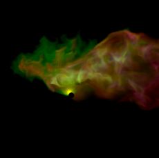
A&A proofs: manuscript no. RFMGRB-2-Application-to-LS5039

by relativistic boosting (see e.g. Dubus et al. 2010) depending
                                                                             0.1
on the orientation of the system. This interplay between the gen-
                                                                                                 C                             Periastron
eration of inverse Compton emission and its absorption by pair-                               SUP Superior= 0.058
                                                                                                            Conjuntion
                                                                                                                                   =0
production together with the phase-dependent relativistic boost-
ing is commonly used to explain the observed anti-correlation of
the HE gamma-ray emission to the X-ray and VHE gamma-ray
fluxes.
Due to the high γγ-opacity, a one-zone model for LS 5039 with                 0                                   Star
a single emitter at the stellar and pulsar wind standoff predicts
non-detectable VHE fluxes at superior conjunction, whereas a

                                                                      [AU]
faint source is still clearly detected. This indicates that the VHE                                                             = 0.9
emitting region is more extended and located farther away from
the star since an alternative explanation via an electromagnetic
cascade initiated by the γγ pair-production turned out to be in-
                                                                                        = 0.45
compatible with the observed spectrum (see e.g. Bosch-Ramon                  0.1
et al. 2008; Cerutti et al. 2010). A plausible second emission

                                                                                                                                     Observer
region is the Coriolis shock, which is formed due to the orbital                                       Inferior Conjunction C
motion of the system (see Bosch-Ramon & Barkov 2011; Bosch-                          = 0.5                     = 0.716     INF
Ramon et al. 2012). Using an analytic approximation to describe                    Apastron
its location, the Coriolis shock was established as a viable site
for particle acceleration and the subsequent production of VHE                                0.1                  0                    0.1
gamma-rays (see, e.g., Zabalza et al. 2013). While such an an-                                             [AU]
alytic two-zone model still oversimplifies the structure of the
WCR, it shows that an approach that contains the precise struc-       Fig. 1. The LS 5039 system as determined by Casares et al. (2005) with
ture of the WCR can take the extended emission region and the         an orbital period of Porb = 3.9 d and an eccentricity of e = 0.35 as-
consequent dilution of γγ-absorption into account very naturally.     suming a stellar mass Mstar = 23 M and pulsar mass Mpulsar = 1.4 M .
To obtain a more realistic picture of the WCR, the pulsar- and        Periastron, apastron and the conjunctions are indicated. Matching the
stellar-wind interaction was investigated numerically using ded-      choices in Aharonian et al. (2006) the orbit is divided in INFC ranging
icated relativistic hydrodynamics (RHD) simulations (see e.g.         from 0.45 < φ < 0.9, and SUPC with 0.9 < φ < 1 and 0 < φ < 0.45.
Lamberts et al. 2013; Bosch-Ramon et al. 2015). These simu-
lations were used in combination with particle transport mod-
els to build more comprehensive emission models with various          gether with the fluid solutions to generate predictions for the
degrees of complexity (see e.g. Dubus et al. 2015; Molina &           non-thermal emission of the system, comprising synchrotron and
Bosch-Ramon 2020). However, these models do not take the              anisotropic inverse-Compton emission with additional modula-
complex dynamic structure of the wind-interaction into account        tion by relativistic boosting and γγ-absorption.
and rely on simplified simulations or analytic reductions of sim-     The present paper is the second in a series of papers. Here, we
ulations.                                                             apply the model presented in Huber et al. (2021) to the LS 5039
In Dubus et al. (2015), the authors solve a Fokker-Plank-type         system, which is a prime candidate for the investigation of fluid
particle-transport equation for accelerated electronic pairs using    models of gamma-ray binaries due to the well know and less
results from a simplified wind-interaction simulation as steady-      complex stellar-wind model as compared to other systems with
state background. This allows for relativistic and anisotropic        stellar disks. With this application, we aim to identify the rel-
effects to be included consistently in the computation of the         evant emission regions in three dimensions and to assess the
generated emission. The wind interaction was simulated in a           impact of fluid dynamics on the radiative output of the system,
non-turbulent setup, symmetric around the binary axis, which is       which has not been possible with previous approaches.
rescaled for different orbital phases. While reducing the compu-      The paper is structured as follows: in Sect. 2 we specify the
tational effort, the assumption of axisymmetry prevents orbital       setup of the simulation; the resulting fluid solution, particle dis-
motion to be taken into account, implying that a Coriolis shock       tributions and predicted emission for LS 5039 are presented in
cannot be formed in such a simulation. Further, with a steady-        Sect. 3; and a summarizing discussion is given in Sect. 4.
state fluid background, the impact of fluid dynamics is neglected.
However, more complex simulations (e.g. Bosch-Ramon et al.
2015) have shown that neither the shock structure nor the down-       2. Simulation setup
stream flow are stationary but depend on the orbital phase and        The LS 5039 system is composed of a massive, O-type star in a
are subject to turbulence arising in the WCR.                         mildly eccentric orbit with, what we assume to be, a pulsar, de-
In Huber et al. (2021) we presented a novel numerical model           spite that no pulsations have been detected, yet. We employ the
for the non-thermal emission of gamma-ray binaries in a pulsar-       orbital solution determined by Casares et al. (2005), with a pe-
wind driven scenario, with which we aim to alleviate some of          riod Porb = 3.9 d and eccentricity e = 0.35. We assume a stellar
the approximations in previous modelling efforts while incor-         mass Mstar = 23 M and a pulsar mass Mpulsar = 1.4 M (similar
porating previous approaches in a self-consistent framework. In       to Dubus et al. 2015), yielding a semi-major axis a = 0.145 AU,
the presented approach the pulsar- and stellar-wind interaction is    apastron distance da = 0.196 AU and periastron distance d p =
treated in a dedicated 3-dimensional relativistic hydrodynamic        0.094 AU, as depicted in Fig. 1.
simulation. The novelty of this approach consists of a simulta-       To simulate the fluid of the stellar and the pulsar wind, we nu-
neous solution of the fluid dynamics and the particle transport       merically solve the equations of special-relativistic hydrodynam-
for the electron-positron pairs, accelerated at the arising shocks.   ics, using a reference frame co-rotating with the average an-
This yields consistent particle distributions, which are used to-     gular velocity of the system Ω = 2π/Porb (see Huber et al.
Article number, page 2 of 14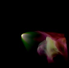
D. Huber et al.: Relativistic fluid modelling of gamma-ray binaries

2021, for more details). The dynamical equations are solved us-                netic might differ in the shocked downstream flow, this approx-
ing the Cronos code (Kissmann et al. 2018). The simulation is                  imation is expected to yield good values at the shocks, which is
performed on a Cartesian grid with dimensions [−1.25, 1.25] ×                  most relevant for the particle injection. For the stellar compan-
[−0.5, 1.5] × [−0.5, 0.5] AU3 , which is homogeneously subdi-                  ion, we assume a luminosity L? = 1.8 × 10⁵ L , temperature
vided into 640 × 512 × 256 spatial cells. The binary orbits in                 T ? = 39000 K and resulting radius R? = 9.3 R (Casares et al.
the x − y plane, with its centre of mass coinciding with the coor-             2005).
dinate origin.
For the simulation of the wind interaction (presented in
Sect. 3.1), we adopted a stellar mass loss rate of Ṁ s = 2 ×                  3. Results
10−8 M yr−1 and a terminal velocity of v s = 2000 km s−1 (Dubus
                                                                               3.1. Fluid structure
et al. 2015). The speed of the pulsar wind is set to v p = 0.99 c,
corresponding to a Lorentz factor of u0 p = 7.08. While this                   In Fig. 2 we show the resulting fluid mass-density for differ-
is smaller than conventional values u0 p ∼ 104 − 106 (see e.g.                 ent orbital phases. An extended wind collision region (WCR)
Khangulyan et al. 2012; Aharonian et al. 2012, and references                  is formed from the stellar- and pulsar-wind interaction, creating
therin), it is still high enough to capture the relevant relativis-            a bow-like shock (hereafter bow shock) on the pulsar side. The
tic effects (Bosch-Ramon et al. 2012). The pulsar mass loss rate               overall shape of the WCR is highly asymmetric and bends in the
Ṁ p = η Ṁuspus is scaled with η = 0.1, yielding a corresponding pul-         direction opposite to the orbital motion due to the Coriolis force
                                                                               acting on the rotating system. The additional force leads to a ter-
sar spin-down luminosity Lsd = 7.55 × 1028 W. Both, the stellar                mination of the pulsar wind on the far side of the system forming
and the pulsar winds, are continuously injected within a spheri-               another shock at the Coriolis turnover (hereafter Coriolis shock).
cal region with radius rinj = 0.08 a around each object, initially             In the downstream region of the Coriolis shock, shocked pulsar
placed in a vacuum. To account for the eccentricity of the orbit,              wind is turbulently mixed with shocked stellar-wind material,
the locations of the injection volumes are updated accordingly                 slowing the flow due to increased mass load (see also Fig. A.1).
after every step of the simulation.                                            Many secondary shocks are formed in the turbulent motion of
The simulation is performed for approximately 1.6 orbits. The                  the fluid, which can re-energize already cooled particles acceler-
first 0.6 orbits are used to initialize the simulation, giving the             ated at other shocks (Bosch-Ramon et al. 2012). In the wings of
slower stellar wind time to populate the computational domain,                 the WCR, the pulsar wind shocked at the bow is reaccelerated to-
which reaches the farthest corner of the simulation box after                  wards its initial Lorentz factor (see also Bogovalov et al. 2008)
tcrossing ≈ 0.45Porb ≈ 1.75 d. The subsequent full orbit is used               until it reaches the turbulently mixed fluid behind the Coriolis
for the scientific analysis.                                                   shock creating an additional shock (hereafter reflected shock in
For the evolution of the accelerated electron-positron pairs, we               analogy to Dubus et al. (2015)) extending diagonally into the re-
solve a Fokker-Planck-type transport equation simultaneously to                gion behind the pulsar (clearly visible at φ ' 0.3 in Fig. 2 and
the fluid interaction using an extension to the Cronos code (Hu-               also Fig. A.2). Features visible in our simulation are in qualita-
ber et al. 2021). For the particles, we use 50 logarithmic bins                tive agreement with previous works (Bosch-Ramon et al. 2015,
in energy covering the range γ ∈ [200, 4 × 10⁸ ]. At the ac-                   see e.g.), validating our fluid model.
celeration sites, identified by a strongly compressive fluid flow              While the Coriolis shock location is in agreement with previ-
∇µ uµ < −10 c/AU, where uµ is the fluids four-velocity, we inject              ous works at periastron, its distance from the pulsar becomes
two particle populations into the simulation: A powerlaw com-                  too large and leaves the computational domain around apastron.
ponent, corresponding to accelerated, non-thermal pairs, and a                 This suggests that the simulation box does not capture enough
Maxwellian component, corresponding to isotropised pairs from                  of the leading edge of the WCR, which therefore cannot sweep
the pulsar wind (see also Dubus et al. 2015). For brevity, we                  up enough dense stellar-wind material to build up the required
will refer to these particles only as electrons for the rest of this           pressure to terminate the pulsar wind.
work. The non-thermal electrons are injected with a spectral in-               The structure of the WCR is strongly influenced by turbulence
dex s = 1.5 and an acceleration efficiency ξacc = 2, determining               developing at the contact discontinuity in the WCR. Next to
                                         µ0 ec
                                                   1/2
the maximum energy γmax = 4π          3
                                        ξacc σT B0      reached by balanc-     the Kelvin-Helmholtz (KH) instabilities triggered by the large
ing diffusive shock acceleration and synchrotron losses with the               velocity shear, the arising turbulence is further increased by
magnetic field strength B0 . We assume a fraction ζePL = 0.45 of               Rayleigh-Taylor (RT) and Richtmeyer-Meshkov (RM) instabil-
the local internal fluid energy and a fraction ζnPL = 4×10⁻³ of the            ities (Bosch-Ramon et al. 2012). This dominantly occurs at the
number of available electrons from the pulsar wind to be injected              leading edge of the WCR (in front of the pulsar with respect to
as non-thermal component. The remaining electrons are injected                 the counter-clockwise orbital motion), because there the high-
as a Maxwellian component. Since the pulsar-wind Lorentz fac-                  density, shocked stellar wind is pressed against the low-density,
tor used in our simulation might be higher in reality, the density             shocked pulsar wind by the Coriolis force (see also Bosch-
of the pair plasma will be overestimated in our simulation. To                 Ramon et al. 2012). We found that the formation of the Coriolis
account for this, we decrease the number of available electrons                shock is influenced by the arising turbulence (see e.g. φ ' 0.8
considered in the injection by a factor ζρ = 5.5 × 10⁻⁴ .                      in Fig. 2), that can cause orbit-to-orbit variations in the WCR
In our simulation, we do not evolve the magnetic field explicitly,             structure.
which makes assumptions on its spatial dependence necessary.                   The development of KH instabilities is strongly suppressed for
Therefore, we conduct the simulations under the assumption that                highly relativistic flows (see e.g. Perucho et al. 2004; Bodo et al.
the magnetic-field energy density in the fluid frame is propor-                2004). Fluctuations can therefore only efficiently grow in the
tional to the internal energy density of the fluid 2µ       B02       p
                                                                = ζb Γ−1 (in   vicinity of the wind standoff, where the shocked pulsar wind is
                                                              0
                                                                               sufficiently slow, having a speed of . c/3, before it is reaccel-
analogy to Barkov & Bosch-Ramon 2018) with ζb = 0.5. This
                                                                               erated. The timescale for advection out of this region therefore
approximation is similar to the one used in Dubus et al. (2015)
                                                                               critically determines the largest modes that can be excited in the
at the location of the shocks. Although the evolution of the mag-
                                                                               system, since the growth-rate for KH instabilities ΓKH ∝ λ−1
                                                                                                                       Article number, page 3 of 14
A&A proofs: manuscript no. RFMGRB-2-Application-to-LS5039
/ kg m 3
10 20 10 18 10 16 10 14 10 12
1.5
1.0
y [AU]
0.5
0.0
=0.193 SUPC =0.289 SUPC =0.393 SUPC =0.489 INFC =0.593 INFC
1.5
1.0
y [AU]
0.5
0.0
=0.689 INFC =0.793 INFC =0.896 INFC =0.993 SUPC =0.089 SUPC
1.0 0.5 0.0 0.5 1.0 1.0 0.5 0.0 0.5 1.0 1.0 0.5 0.0 0.5 1.0 1.0 0.5 0.0 0.5 1.0 1.0 0.5 0.0 0.5 1.0
x [AU] x [AU] x [AU] x [AU] x [AU]
Fig. 2. The fluid’s mass density in the orbital plane for different orbital phases, indicated by the inset annotations. An extended WCR is formed
due to the interaction of the pulsar (blue) and stellar (orange) wind. The reference frame is corotating with counter-clockwise orbital motion. The
labels (INFC/SUPC) correspond to respective parts of the orbit as defined in Fig. 1. The boundaries of the inner, middle and far region (further
discussed in the text) are indicated by the dashed and dotted lines, respectively.
decreases with larger wavelengths (see Bodo et al. 2004; Lam- instabilities becomes more efficient because ΓKH ∝ λ−1 .
berts et al. 2013). The maximum wavelength of fluctuations In our simulation, we do not consider any feedback of the ac-
that can be excited in the presented system is on the order of celerated particles onto the fluid dynamics. Because the non-
λmax ∼ 0.1 AU (assuming a region extension of ∼ 0.3 AU and an thermal electrons contribute a significant fraction to the over-
average advection velocity of ∼ 0.5 c). all energy density, their cooling will result in a decrease of the
The pulsar-wind Lorentz factor used in our simulation is lower fluid’s pressure supporting the WCR. Consequently, when tak-
than typically assumed values ∼ 104 −106 , due to numerical lim- ing such feedback into account, the WCR will be less extended
itations. A higher pulsar wind Lorentz factor will yield a faster and might thus be more susceptible to thin-shell instabilities (as
reacceleration (Bosch-Ramon et al. 2012) when the shocked pointed out by Dubus et al. 2015) as it was seen in the case of
flow is expanding in the wings and might therefore reduce the ad- colliding-wind binaries by Reitberger et al. (2017). The consid-
vection timescale and shift the maximum wavelength of growing eration of such effects is left for future work.
fluctuations to smaller values. However, Bogovalov et al. (2008)
have found that even in the ultra-relativistic limit, the shocked
pulsar-wind flow remains slow near the head of the bow-shock 3.2. Particle distribution
up to scales of the orbital separation for our choice of η. This
is mainly a consequence of the bow-like geometry of the WCR, Since the timescale for the particle populations to reach a quasi-
causing the upstream incident angle with the shock normal to steady state (by reaching the limits of the computational domain
be small over a wide part of the head of the bow shock leading and/or by cooling) is orders of magnitudes smaller than the or-
to a strongly slowed downstream flow. Further, the flow cannot bital timescale we do not perform a particle transport simulation
expand rapidly there, keeping the reacceleration at a moderate for the full timespan of the fluid simulation. Instead, to reduce
level. The reacceleration only becomes more important farther the computational effort, we restart a particle transport simula-
out, where the opening angels of the pulsar-wind shock and the tion on previously obtained fluid solutions for the 10 chosen or-
contact discontinuity approach their asymptotic values. The ex- bital phases shown in Fig. 2. We perform these simulations for
tent of the unstable region hence cannot go below the scales on t = 1.11 h allowing the injected electrons to populate the system.
the order of the orbital separation regardless of the pulsar-wind To simulate the energetic evolution of the electrons, we employ
Lorentz factor, thus only slightly changing the estimates from the semi-Lagrangian scheme described in Huber et al. (2021).
above. Even in the ultra-relativistic limit, KH instabilities are For this, we use the same timestep as for the preceding hydro-
therefore still expected to grow and the overall structure of the dynamic step that is mainly determined by the speed of the un-
WCR should not change significantly. shocked pulsar-wind and the spatial resolution yielding typical
For our setup, we have found in numerical tests (simulating the values of ∆t ∼ 0.8 s. Due to the semi-Lagrangian nature of the
decay of shear flows as described by Ryu & Goodman 1994) scheme, an additional reduction of the timestep depending on the
that damping by numerical viscosity Γdamp ∝ λ−3 dominates over energy resolution is not required to maintain stability.
the KH growth-rate (estimated from Bodo et al. 2004) for short- In Fig. 3 and Fig. 4 we present the resulting electron distribu-
wavelength fluctuations with λ . 10−2 AU. The chosen reso- tions for different orbital phases at two energies, dominantly
lution, therefore, allows the growth of fluctuations in the range populated by Maxwellian and power-law electrons, respectively.
10−2 AU. λ . 10−1 AU (as seen in Fig. 2), where the latter The relevant shock structures are imprinted in the electron dis-
will have the biggest impact on the WCR. This also implies that tributions. This is especially visible for particles at higher ener-
future higher-resolution simulations will extend the range of tur- gies, which are quickly cooled through synchrotron and inverse
bulence to smaller spatial scales for which the driving by KH Compton losses. Due to increased losses, they remain much
Article number, page 4 of 14D. Huber et al.: Relativistic fluid modelling of gamma-ray binaries
( = 3.11 × 10³) / m 3
102 103 104 105 106
1.5
1.0
y [AU]
0.5
0.0
=0.193 (0) SUPC =0.289 (1) SUPC =0.393 (2) SUPC =0.489 (3) INFC =0.593 (4) INFC
1.5
1.0
y [AU]
0.5
0.0
=0.689 (5) INFC =0.793 (6) INFC =0.896 (7) INFC =0.993 (8) SUPC =0.089 (9) SUPC
1.0 0.5 0.0 0.5 1.0 1.0 0.5 0.0 0.5 1.0 1.0 0.5 0.0 0.5 1.0 1.0 0.5 0.0 0.5 1.0 1.0 0.5 0.0 0.5 1.0
x [AU] x [AU] x [AU] x [AU] x [AU]
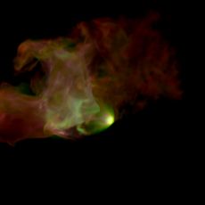
Fig. 3. Differential particle number density for electrons with γ = 3.11 × 10³ in analogy to Fig. 2. The arrows indicate the projected direction to
an observer at Earth. For clarity, we show only 5 orders of magnitude below the highest value - the blue regions correspond to those with lower
values.
( = 1.05 × 10⁷) / m 3
10 6 10 5 10 4 10 3 10 2
1.5
1.0
y [AU]
0.5
0.0
=0.193 (0) SUPC =0.289 (1) SUPC =0.393 (2) SUPC =0.489 (3) INFC =0.593 (4) INFC
1.5
1.0
y [AU]
0.5
0.0
=0.689 (5) INFC =0.793 (6) INFC =0.896 (7) INFC =0.993 (8) SUPC =0.089 (9) SUPC
1.0 0.5 0.0 0.5 1.0 1.0 0.5 0.0 0.5 1.0 1.0 0.5 0.0 0.5 1.0 1.0 0.5 0.0 0.5 1.0 1.0 0.5 0.0 0.5 1.0
x [AU] x [AU] x [AU] x [AU] x [AU]
Fig. 4. Same as Fig. 3, but for γ = 1.05 × 10⁷ .
more confined to their injection sites. Lower-energetic electrons, normalisation but also the shape of the spectrum is a function
in comparison, dominantly lose energy via adiabatic losses and of the orbital phase, considering the location of the peak in the
are therefore cooled on longer timescales, populating a much Maxwellian electrons, the break in the power-law tail and the
larger spatial domain. Next to the bow and Coriolis shocks also maximum energies reached. Furthermore, it shows that a higher
the reflected shock and the countless secondary shocks in the tur- electron density is reached after periastron, which is not intuitive
bulent downstream region behind the pulsar are manifestly vis- at first glance.
ible. In our simulation, radiative losses are highest at the wind This becomes more apparent in Fig. 6, where we show the tem-
standoff, which limits the maximum electron energy reached in poral evolution of the electron distribution integrated over the
the acceleration and the length-scales over which non-thermal computational volume at selected energies. Apparently, the num-
electrons are cooled afterwards. At the Coriolis shock, both the ber of electrons in the computational volume lags behind the or-
magnetic and stellar-radiation field are weaker in comparison bit, i.e. the minimum amount of electrons is reached after apas-
and the highest particle energies of the simulation are reached tron and the maximum after periastron.
(see Fig. 5). This delay is caused by the inertia of the fluid. The WCR needs a
In Fig. 5 we show the spectral energy distribution of the elec- certain time to build up or dissipate its pressure, which critically
trons integrated over the computational volume. The contribu- determines the amount of electrons accelerated at the shocks.
tions of the Maxwellian and the power-law electrons can be eas- This phenomenon can only be seen in approaches that treat the
ily distinguished as they dominate the energy range below and particle transport together with the underlying fluid. The varying
above γ ∼ 2 × 10⁴ , respectively. It is apparent that not only the size of the shocks counteracts parts of this effect by shrinking
Article number, page 5 of 14A&A proofs: manuscript no. RFMGRB-2-Application-to-LS5039
1044 index and the acceleration timescale depend on the shock’s com-
= 0.193
= 0.393 pression ratio, magnetic obliquity, and up- and downstream fluid
= 0.593 velocities (see e.g. Keshet & Waxman 2005; Takamoto & Kirk
= 0.793 2015). In future efforts, the current model can be extended to
= 0.993
1043 investigate different acceleration mechanisms.
2 dN/d
3.3. Emission
1042 In this section, we present the simulation results for the non-
thermal emission spectrum and lightcurves of LS 5039. They
are produced in a post-processing step, using the previously ob-
tained particle distributions (see Sect. 3.2) and fluid solutions
1041 (see Sect. 3.1). We, therefore, generate direct predictions on the
103 104 105 106 107 108 initially spelt-out set of model-parameters (see Sect. 2).
For the computation of the inverse Compton emission, we treat
Fig. 5. Spectral energy distribution of electrons integrated over the the stellar photon field as monochromatic, whereas for the γγ-
computational domain for different orbital phases (colour-coded, solid). absorption a full blackbody spectrum is considered. In both
For φ = 0.393, the contributions of the inner (dashed), middle (dash- cases, the source is treated as an extended sphere. We compute
dotted), and outer (dotted) region are shown, respectively, as an exam- the emission for two different system inclinations i = 30◦ and
ple. i = 60◦ .
In our approach, it is no longer straightforward to separate the
= 4.1 × 10² emission produced through particles accelerated at the different
= 9.8 × 10² shocks as it was possible in previous works (e.g. Dubus et al.
= 2.3 × 103
= 5.6 × 10³
2015), since the downstream flows are turbulently mixed which
1043 = 1.3 × 10⁴ was previously neglected. To obtain a basic understanding of the
[m 3]
= 3.2 × 10⁴ location dependence of the emission we subdivide the computa-
= 7.6 × 10⁴ tional volume into three regions (henceforth called inner, middle,
= 1.8 × 10⁵
2 dN/d
= 4.3 × 10⁵ and far region, respectively), which are separated at distances
= 1.0 × 10⁶ of 1.2 d and 3.5 d from the binaries centre of mass, where d is
1042 = 2.5 × 10⁶ the time-dependent orbital distance (see Fig. 2). In Sect. 3.3.1
= 5.9 × 10⁶ we present the predicted emission spectra followed by a more
periastron
apastron
apastron
= 1.4 × 10⁷
detailed discussion for individual energy-bands in Sect. 3.3.2,
supc
supc
infc
infc
Sect. 3.3.3 and Sect. 3.3.4. A projection map of the emission is
0.0 0.5 1.0 0.5 1.0 discussed in Sect. 3.5.
Orbital Phase
Fig. 6. Temporal evolution of the spectral energy distribution of en- 3.3.1. Emission spectrum
ergetic electrons integrated over the computational domain for selected
energies (colour-coded). For better visualisation, we show the same data In Fig. 7 we show the resulting spectral energy distributions of
for two orbits. photons emitted for two different inclinations of the system, in-
tegrated over different orbital phases: for comparison to observa-
and enlarging the acceleration sites at periastron and apastron, tions, the orbit has been split into two parts, INFC and SUPC as
respectively, which is, however, not dominant in our simulation. defined in Aharonian et al. (2006) (see Fig. 1). To compute the
The power injected at the shocks reaches its maximum at φ ' 0.2 average spectra we integrate the simulated ones using piece-wise
in our simulation, suggesting an expected peak in the integrated linear interpolations in time.
electron distribution with the same delay. The spectral features of the particle population leave clear im-
We find, however, that this delay is energy-dependent. While the prints in the emission spectrum. Ranging from X-rays up to LE
number of higher-energetic electrons peaks as expected around gamma-rays the spectrum is dominated by synchrotron emission
φ ' 0.2, the number of lower-energetic ones peaks earlier at generated by electrons at the power-law tail of the spectrum,
φ ' 0.1 (see Fig. 6). This behaviour originates in the turbu- dominantly produced in the inner region. The same population
lent flow behind the pulsar formed earlier around the periastron of electrons is responsible for the inverse Compton scattering of
passage, which leads to a pile-up of electrons at lower energies stellar UV photons to the VHE gamma-ray regime, although, the
yielding an earlier peak in their evolution. This effect is not rele- relative contributions of the individual regions to the VHE emis-
vant for electrons at higher energies since they are cooled much sion is not constant but varies along the orbit. The emission in
faster through radiative losses. Consequently, these particles are the HE gamma-ray regime is also produced through the inverse
more confined to the shocks preventing a pile-up and leaving Compton process, however, by the lower-energetic Maxwellian
their number density more directly affected by the acceleration electrons in the inner region of the system.
process.
We treat both the spectral slope and the acceleration efficiency 3.3.2. X-Rays and LE gamma-rays
as free model parameters since the specifics for particle accel-
eration in gamma-ray binaries have not been firmly identified, For the chosen set of parameters, the synchrotron emission pre-
yet. In this phenomenological approach, we treat all acceleration dicted by our model is able to explain the observed X-ray to LE
sites the same, which might not be the case in reality. For exam- gamma-rays emission spectrum (see Fig. 7). This was not pos-
ple, in the case of diffusive shock acceleration, both the spectral sible in previous studies (Dubus et al. 2015; Molina & Bosch-
Article number, page 6 of 14D. Huber et al.: Relativistic fluid modelling of gamma-ray binaries
10 9
i = 30 INFC i = 60 INFC
F [TeV s 1 cm 2]
10 10
10 11
10 12
10 13
i = 30 SUPC i = 60 SUPC
F [TeV s 1 cm 2]
10 10
10 11
10 12
10 13
104 106 108 1010 1012 1014 104 106 108 1010 1012 1014
[eV] [eV]
Fig. 7. Spectral energy distribution of the emission predicted by our model for LS 5039 for different parts of the orbit and inclinations of
the system. Different radiative processes are colour-coded: synchrotron (green), inverse Compton (orange), inverse Compton attenuated by γγ-
absorption (red) and total (black). The contributions to the total emission from the inner (dashed), middle (dashed-dotted) and far (dotted) region
are shown separately (for a description of the regions see the main text). The model predictions are shown together with observations in soft X-rays
(Takahashi et al. 2009), LE (Collmar & Zhang 2014), HE (Hadasch et al. 2012) and VHE (Aharonian et al. 2006) gamma-rays. Results are shown
for different parts of the orbit as defined in Fig. 1 with INFC on the left and SUPC on the right column. In the top row results are shown for an
inclination i = 30◦ of the orbital plane, while in the second row, the results for an inclination i = 60◦ are presented.
Ramon 2020). Synchrotron emission dominates up to ∼ 10 MeV, (Dubus et al. 2015). These problems, therefore, highlight the ne-
with a spectral cutoff approximately constant over the orbit. The cessity for a more sophisticated magnetic field description in fu-
electrons emitting at the LE cutoff are at the highest end of the ture modelling.
power-law tail, accelerated at the apex of the bow shock. These We also investigated the effects of different magnetic field mod-
particles are strongly confined to shocks and, thus, rely on our els, such as a passively advected magnetic energy density wB
injection model and the conditions directly at the shock. This injected together with the pulsar wind and/or a magnetic field
means that the synchrotron cutoff directly depends on two fac- aligned with the fluid bulk motion. The injected magnetic energy
tors: the maximum electron energy (see Sect. 2) and the maxi- density is scaled with the injected kinetic energy density as wB =
mum photon energy produced through the synchrotron process. Ṁ p c2 u0
σ 4πr2 u pp with the pulsar wind magnetisation fraction σ, yielding
Both quantities only depend on the magnetic field, however,
the magnetic field in the laboratory frame B = 2µ0 wB . We
p
counteracting each other leading to a constant synchrotron cut-
off. found little difference in the resulting emission spectra when us-
While the model predictions closely resemble the X-ray and ing these alternative models for similar magnetic field strengths,
LE gamma-ray observations at INFC, the X-ray flux is over- still yielding disagreement with the predicted X-ray lightcurve.
predicted at SUPC. This deviation is also manifest in the X- For larger inclination angles (see the right column in Fig. 8), rel-
ray lightcurve (see the first row of Fig. 8). Instead of the ob- ativistic boosting becomes more important. This decreases the
served correlation with VHE gamma-rays, the predicted X-ray X-ray flux at superior conjunction while increasing it at inferior
lightcurve is correlated with the HE gamma-ray flux. This is conjunction, which is better resembling the features of the ob-
caused by the still simplistic magnetic field description em- served lightcurve.
ployed in our model: Since the magnetic field strength directly
scales with the fluid pressure, its maximum at the bow shock is
3.3.3. HE gamma-rays
reached shortly after periastron. In addition, also electron accel-
eration is increased in this part of the orbit. The combined effects While the overall spectral shape and the flux of the predicted
lead to a modulation of the synchrotron emissivity that dom- HE emission are in good agreement with observations at SUPC,
inates over the one introduced by relativistic boosting, which the predictions prove to be problematic at INFC (see Fig. 7).
was argued to be the dominant source of variability in this band There, the predicted HE flux drops by approximately one order
Article number, page 7 of 14A&A proofs: manuscript no. RFMGRB-2-Application-to-LS5039
i = 30 i = 60
SUPC INFC SUPC INFC SUPC INFC SUPC INFC
apastron
periastron
apastron
apastron
periastron
apastron
supc
supc
supc
supc
infc
infc
infc
infc
2
]
11 ergcm 2 s 1
F1 10keV
1
10
0
[
]
1
10 7 phcm 2 s
4
F0.2 3GeV
2
[
0
4
]
12 phcm 2 s 1
3
F > 1TeV
2
1
10 [
0
0.0 0.2 0.4 0.6 0.8 0.0 0.2 0.4 0.6 0.8 0.0 0.0 0.2 0.4 0.6 0.8 0.0 0.2 0.4 0.6 0.8 0.0
Orbital Phase Orbital Phase
Fig. 8. Emission lightcurves predicted by our model for LS 5039 for different energy bands and inclinations of the system. The contributions
from the inner (orange, dashed), middle (green, dashed-dotted) and far (red, dotted) region together with their sum (blue, solid) are shown (for a
description of the regions see the main text). For better visualisation, we show the same data for two orbits. The results are shown for different
energy bands together with observations in indivdual rows (from top to bottom): Soft X-rays (1 − 10 keV, Takahashi et al. 2009), HE (0.2 − 3 GeV,
Hadasch et al. 2012) and VHE (> 1 TeV, Aharonian et al. 2006) gamma-rays. In the left column results are shown for an inclination i = 30◦ of the
orbital plane, while in the right column, the results for an inclination i = 60◦ are presented. In addition to the orbital phases described in the main
text, we show 3 more lightcurve points at φ ∼ 0.55, 0.65, 0.85. The error bars indicate the variability introduced by turbulence (see Sect. 3.4).
of magnitude and the spectrum is shifted towards lower ener- for the Maxwellian electron distribution to avoid overestimation
gies leaving the fluxes underpredicted. These changes in the flux of the flux at SUPC.
are mainly caused by the anisotropic inverse Compton scatter- The discrepancy is also apparent in the predicted HE lightcurves
ing cross-section, which grows with scattering angle. At phases (see the second row in Fig. 8), showing a phase-independent
around superior conjunction, stellar photons have to be scat- underestimation with respect to the observations. Disregarding
tered by a larger angle to reach the observer as compared to the constant underprediction, the lightcurve for an inclination
inferior conjunction. Consequently, the highest and lowest in- of i = 30◦ is in good agreement with observations. For the
verse Compton fluxes relate to these phases, respectively. The higher inclination angle, the inverse Compton anisotropy leads
anisotropic scattering further causes the shift in energy, yield- to a steep rise in emission at superior conjunction, while further
ing higher scattered photon energies for larger scattering angles. reducing the flux at phases around apastron and inferior conjunc-
Both effects can also be seen by comparing the different inclina- tion.
tion angles (e.g. see Fig. 7). Inverse Compton emission by relativistic Maxwellian pairs in the
An additional modulation is generated by the changing stellar cold pulsar wind might yield another contribution in this energy
seed radiation field density induced by the varying distance of band. The current model does not take this contribution into ac-
the bow shock apex to the star, with the maximum and minimum count explicitly, since the required ultra-relativistic pulsar wind
stellar photon density at periastron and apastron, respectively. Lorentz factor u0 p ∼ 5000 cannot be captured by our numeri-
Due to the geometry of the LS 5039 orbit, the periastron passage cal methods. The produced spectra, however, strongly resemble
occurs very close to superior conjunction leading this modula- the ones produced by the Maxwellian electrons injected at the
tion to add to the former one. shocks in our model (see Takata et al. 2014). Due to this de-
The underestimation of the HE gamma-ray flux at INFC suggests generacy, the latter effectively captures this contribution in our
a missing component in our broadband emission model, which modelling.
could arise from the magnetospheric emission of the pulsar as
suggested e.g. by Takata et al. (2014). This process can natu-
rally account for the phase-independent spectral cutoff of the HE 3.3.4. VHE gamma-rays
emission at energies of a few GeV. To accommodate this emis- In contrast to the HE gamma-ray emission, the flux at VHE is
sion within our modelling one has to find a new set of parameters heavily attenuated by γγ-absorption, introducing an additional
Article number, page 8 of 14D. Huber et al.: Relativistic fluid modelling of gamma-ray binaries
Flux Contribution conjunction is extended over a large volume behind the pulsar
10 2 10 1 100 (see Fig. 9). In particular, it extends to the edges of the compu-
tational volume, suggesting that a fraction of the emission is lost
1.0 by particles leaving the domain. A larger computational domain
is required to address this issue, which goes beyond the scope of
0.8 available computational resources.
Orbital Phase
infc For a system inclination of i = 60◦ we find a sharp peak in the
INFC
0.6 100 GeV
predicted VHE lightcurve at φ ' 0.55 (see third row in Fig. 8).
i = 60 At this phase, the observer’s line of sight is aligned with the lead-
0.4 ing edge of the shocked pulsar wind flow, yielding a drastically
increased photon flux due to relativistic boosting (which can also
0.2
SUPC
be seen at the bottom of Fig. 9) that is incompatible with obser-
supc vations. The trailing edge of the WCR is crossed by the observer
1.0 between φ ' 0.8 and φ ' 0.9 in our simulation, showing no
peaked emission.
0.8
Orbital Phase
infc
INFC
3.4. Turbulence-induced variability
0.6 10 TeV
i = 60 To assess the impact of short-term variability on the system’s ra-
0.4 diative output introduced by turbulence, we evolved the particle
SUPC distributions presented in Sect. 3.2 for more time and recom-
0.2 puted the emission. After the initial convergence time of t0 =
supc 1.11 h, we investigated the particle distributions at tn = t0 + n · ∆t,
0.0 0.2 0.4 0.6 0.8 1.0 1.2 1.4 with ∆t = 0.14 h and n = 0, 1, 2, 3, 4. This time increment ∆t is
Radial Distance [AU] sufficiently longer than the growth-timescale of KH instabilities
(see also Sect. 3.1) for the different solutions to be uncorrelated.
Fig. 9. Relative contribution to the radiation emitted at a given orbital This procedure was repeated for a range of orbital phases, for
phase from spherical shells around the system’s centre of mass (with a which we computed the average and the standard deviation from
thickness of 0.05 AU) at two different energies. For clarity we present the five obtained emission solutions and showed the results in
the results only for a system inclination of i = 60◦ ; the resulting maps Fig. 8.
qualitatively agree with those for an inclination of i = 30◦ . We termi- We found that turbulence introduces variability depending on or-
nate the analysis at r = 1.5 AU, where the farthest edge of the compu-
tational volume is reached. Relevant orbital phases are annotated (see
bital phase and photon energy with variability levels of several
also Fig. 1). per cent, reaching ∼ 17% for the HE flux around superior con-
junction and ∼ 12% for the VHE flux around inferior conjunc-
tion. Most of the variability is apparent in the inner and middle
region, which is expected since these regions are most directly
line-of-sight dependent modulation. The observed spectral fea- affected by instabilities formed at the contact discontinuity. Al-
tures and the temporal characteristics are well recovered by our though turbulence introduces visible flux fluctuations, they are
model with a high energy cutoff in excellent agreement with ob- still considerably smaller than orbital variations and thus do not
servations and a pronounced anti-correlation to the HE gamma- dominate the resulting lightcurves.
ray emission, as shown in Fig. 7 and the third row in Fig. 8, Lastly, we found that the pulsar-wind shock structure is influ-
respectively. enced by turbulence developing at the stellar-wind shock on
Due to γγ-absorption, the VHE-flux, especially from the inner longer timescales (see Sect. 3.1). This has an effect on the vari-
region, is strongly reduced for all phases (see Fig. 7). At INFC, ability on orbital timescales and is expected to introduce orbit-
the larger inclination of i = 60◦ is favourable because the ab- to-orbit variations, which will be studied in the future when more
sorption is weakened by smaller scattering angles as compared computational resources become available.
to i = 30◦ . Here, the dominant part of the emission is produced
in the middle region with strong relativistic boosting, leading to
a hard spectrum as seen in observations. The increased contribu- 3.5. Emission map
tion of this region around inferior conjunction can also be seen For better visualisation of the emission produced in LS 5039 we
more directly in Fig. 9 where we illustrate the relative contri- show a composite, false-colour emission map in Fig. 10 as it
bution to the gamma-ray flux as a function of distance from the would be seen with a perfect angular resolution at Earth. The im-
binary’s centre of mass. print of the fluid-structure is clearly visible, exhibiting the bow
In the 100 GeV to 1 TeV range, where the γγ-absorption is most shock and the turbulent downstream region behind the pulsar
pronounced, the flux is underpredicted with respect to obser- around periastron. At φ ' 0.1 the star is eclipsing parts of the
vations for SUPC. At phases around superior conjunction, the emission region occluding a circular region in the map.
emission produced at both the inner and the middle region is al-
most completely attenuated by absorption, as shown in Fig. 9,
leaving the radiation to be dominantly produced in the far region 4. Summary and discussion
of the system. The predicted fluxes, however, are too small to
reproduce observations around periastron and superior conjunc- In this work, we present the application of a novel numerical
tion (see the third row in Fig. 8), in our simulations. We found model for gamma-ray binaries (Huber et al. 2021) to the LS 5039
that the region that dominates the flux reaching the observer in system. We specifically choose this system for its broad obser-
the energy range most affected by γγ-absorption around superior vational coverage, known orbital parameters and comparison to
Article number, page 9 of 14A&A proofs: manuscript no. RFMGRB-2-Application-to-LS5039
X-Ray diff. Energy Flux @ 13 keV [TeV s 1 mas 2 cm 2] HE diff. Energy Flux @ 1.2 GeV [TeV s 1 mas 2 cm 2] VHE diff. Energy Flux @ 1.6 TeV [TeV s 1 mas 2 cm 2]
10 13 10 12 10 11 10 10 10 9 10 8 10 13 10 12 10 11 10 10 10 9 10 8 10 13 10 12 10 11 10 10 10 9 10 8
0.4 =0.187 =0.284 =0.387 =0.484 =0.587
0.2
y [mas]
0.0
0.2
0.4
0.4 =0.684 =0.787 =0.891 =0.987 =0.084
0.2
y [mas]
0.0
0.2
0.4
0.4 0.2 0.0 0.2 0.4 0.4 0.2 0.0 0.2 0.4 0.4 0.2 0.0 0.2 0.4 0.4 0.2 0.0 0.2 0.4 0.4 0.2 0.0 0.2 0.4
x [mas] x [mas] x [mas] x [mas] x [mas]
Fig. 10. Projection of the predicted emission from LS 5039 for different orbital phases as defined with an orbital plane inclination of i = 60◦ . The
differential energy flux is shown for distinct energy bands as indicated by the colour bars. For better visualisation, the upper limit of the colour
bars has been set two orders of magnitude lower than the maximum HE gamma-ray flux.
previous modelling efforts. Dubus et al. 2015) our simulation predicts that the synchrotron
Our simulations of the wind interaction in this system show an emission connects the X-ray emission to the LE gamma-ray
extended, asymmetric WCR bent by the orbital motion, exhibit- emission. We attribute this result to the different WCR geom-
ing a strong bow-like pulsar-wind shock and a Coriolis shock etry, affecting relativistic boosting, and our improved treatment
behind the pulsar. With our approach, it is, for the first time, of the star as an extended photon source, leading to increased γγ-
possible to consistently account for the complex dynamic shock absorption. Similar to previous studies (e.g. Dubus et al. 2015;
structure in the particle transport model. Next to the bow and Molina & Bosch-Ramon 2020), we find that a hard spectral in-
Coriolis shock, this also includes the reflection shock (formed dex of s = 1.5 is required for the electron acceleration to describe
where the downstream plasma of bow and Coriolis shocks col- the observations. The predicted spectra underestimate the flux in
lide) and the secondary shocks, arising in the turbulent down- the HE gamma-ray band, presumably lacking a contribution by
stream medium of the Coriolis shock. The resulting structures the magnetospheric emission of the pulsar (Takata et al. 2014).
are in agreement with the ones observed in previous simulations While the inner region (< 1.2 orbital separations d from the sys-
(see Bosch-Ramon et al. 2015) , although the Coriolis shock is tem’s centre of mass) provides the bulk of the emission from X-
not formed in the numerical domain at phases around inferior rays to HE gamma-rays, the middle and far regions (1.2 − 3.5 d
conjunction. This is caused by the computational domain being and > 3.5 d, respectively) are especially relevant for the emis-
to small to capture enough of the leading edge of the WCR to sion in the VHE band mainly due to relativistic beaming and γγ-
reach the required pressure to terminate the pulsar wind at the absorption. Our conclusions contrast the assessment by Molina
respective phases. In simulations with a larger computational do- & Bosch-Ramon (2020), who found the far region to be the
main, the Coriolis shock is expected to reappear - possibly so dominant emitter for all energies and orbital phases. This di-
close to the pulsar that it would be within the extents of the cur- rectly relates to different assumptions regarding the injection of
rent computational domain. non-thermal electrons in the system. While we assume the same
We find that the extrema of the fluid’s internal energy do coin- fraction of the fluid’s internal energy density to be converted
cide with orbital extrema, as assumed by previous studies (see to non-thermal electrons at all shocks, Molina & Bosch-Ramon
e.g. Dubus et al. 2015; Zabalza et al. 2013; Takata et al. 2014). (2020) assume that a significantly larger fraction of the pulsar’s
This affects the resulting particle distributions since most of the spindown-luminosity is converted at the Coriolis shock than at
models, including the presented one, scale the amount and en- the bow-shock, which is not the case how we perform our simu-
ergetics of accelerated electrons with the available internal fluid lation.
energy. This results in a delay of the electron density extrema of Our model predicts significant orbital modulation in all en-
∆φ ' 0.1 − 0.2 in our model depending on their energy. This ergy bands originating mainly through the anisotropic inverse-
delay also translates to the production of radiation, however, it Compton process, relativistic boosting, and changing proper-
is compensated in parts by the onset of relativistic deboosting at ties of the WCR. While the predicted HE to VHE gamma-ray
superior conjunction (shortly after periastron) in the case of LS lightcurves agree with observations, the simulations fail to re-
5039. produce the observed orbital X-ray and LE gamma-ray modu-
Our model reproduces the main spectral features of the ob- lation. Instead of the observed correlation with VHE gamma-
served emission from LS 5039 ranging from soft X-rays to rays, a correlation with the HE band is predicted. We attribute
VHE gamma-rays, further substantiating a wind-driven interpre- this to the rather simplistic magnetic field model, i.e. scaling the
tation of gamma-ray binaries. In contrast to previous studies (e.g. magnetic energy density with the fluid pressure, which varies
Article number, page 10 of 14D. Huber et al.: Relativistic fluid modelling of gamma-ray binaries
strongly across the orbit and is responsible for the dominant ativistic boosting. This prevents the formation of a second peak
modulation in the synchrotron emissivity. Such a model has been in the VHE lightcurve around φ ∼ 0.85 seen in previous works
employed in previous studies using a semi-analytical description with a more simplified prescription of the WCR for higher incli-
for the emitting particles (e.g. Barkov & Bosch-Ramon 2018), nations (Dubus et al. 2015). Such a second peak is not visible in
but it seems to be increasingly incompatible with our more de- related observations.
tailed particle transport model, emphasising the need for a more In this study, we showed the feasibility of a combined fluid and
sophisticated approach. This could be realised for example by particle-transport simulation for predicting the radiative output
an extension of the presented model to relativistic magneto- of gamma-ray binaries. Future extensions of this model as dis-
hydrodynamics. With this, it will be possible to take the impact cussed shall lead to a better representation of the observations of
of the non-negligible magnetic field onto the fluid dynamics into LS 5039 and will be applied to other well-observed gamma-ray
account, yielding a more realistic picture of the magnetic field binaries.
strength and direction, enabling more realistic injection models Acknowledgements. The computational results presented in this paper have been
and the consideration of anisotropic synchrotron emission. achieved (in parts) using the research infrastructure of the Institute for Astro-
At INFC, the middle region produces the dominant contribution and Particle Physics at the University of Innsbruck, the LEO HPC infrastruc-
to the VHE gamma-ray spectrum due to relativistic boosting, al- ture of the University of Innsbruck, the MACH2 Interuniversity Shared Mem-
ory Supercomputer and PRACE resources. We acknowledge PRACE for award-
lowing a hard spectral index to be maintained. We note that the ing us access to Joliot-Curie at GENCI@CEA, France. This research made
Coriolis shock is not present in the simulation for most of the use of Cronos (Kissmann et al. 2018); GNU Scientific Library (GSL) (Galassi
corresponding phases, as mentioned in the beginning. Its pres- 2018); matplotlib, a Python library for publication quality graphics (Hunter
ence in larger simulations is expected to reduce the size of the 2007); and NumPy (Van Der Walt et al. 2011). We thank the anonymous ref-
bow shock wings, where this relativistically boosted emission is eree for the thoughtful comments and suggestions that allowed us to improve
our manuscript.
originating, which might lead to a softening of the spectrum.
At superior conjunction, a significant part of the VHE gamma-
ray emission is produced by electrons in the far region of the
system due to the weakened impact of γγ-absorption. However, References
emitting particles are lost at the boundaries of the simulation. Abdo, A. A., Ackermann, M., Ajello, M., et al. 2009, ApJ, 706, L56
We suspect this to be the main reason for the underestimation of Aharonian, F., Akhperjanian, A. G., Aye, K. M., et al. 2005, Science, 309, 746
the SUPC flux in the 100 GeV to 1 TeV range and the underesti- Aharonian, F., Akhperjanian, A. G., Bazer-Bachi, A. R., et al. 2006, A&A, 460,
mation of the VHE lightcurve around periastron to superior con- 743
Aharonian, F. A., Bogovalov, S. V., & Khangulyan, D. 2012, Nature, 482, 507
junction. These issues and the missing Coriolis shock at some Barkov, M. V. & Bosch-Ramon, V. 2018, MNRAS, 479, 1320
orbital phases can be addressed by employing a larger computa- Bodo, G., Mignone, A., & Rosner, R. 2004, Phys. Rev. E, 70, 036304
tional volume. Bogovalov, S. V., Khangulyan, D. V., Koldoba, A. V., Ustyugova, G. V., & Aha-
We found that turbulence formed in the wind interaction in- ronian, F. A. 2008, MNRAS, 387, 63
Bosch-Ramon, V. & Barkov, M. V. 2011, A&A, 535, A20
troduces sub-orbital variability in the systems radiative output Bosch-Ramon, V., Barkov, M. V., Khangulyan, D., & Perucho, M. 2012, A&A,
on the levels of several per cent on average, reaching up to 544, A59
∼ 20 per cent for certain orbital phases and photon energies. Bosch-Ramon, V., Barkov, M. V., & Perucho, M. 2015, A&A, 577, A89
The introduced variations in the flux, however, are still con- Bosch-Ramon, V. & Khangulyan, D. 2009, International Journal of Modern
Physics D, 18, 347
siderably smaller than those on orbital timescales. On longer Bosch-Ramon, V., Khangulyan, D., & Aharonian, F. A. 2008, A&A, 489, L21
timescales, turbulence is expected to introduce orbit-to-orbit Casares, J., Ribó, M., Ribas, I., et al. 2005, MNRAS, 364, 899
variations, which cannot be studied from the single simulated Cerutti, B., Malzac, J., Dubus, G., & Henri, G. 2010, A&A, 519, A81
Collmar, W. & Zhang, S. 2014, A&A, 565, A38
orbit. This shows the need for further investigations on larger Dubus, G. 2006, A&A, 451, 9
timescales and a larger spatial domain. Dubus, G. 2013, A&A Rev., 21, 64
Both investigated inclinations of the orbital plane yield fluxes Dubus, G., Cerutti, B., & Henri, G. 2008, A&A, 477, 691
that are more or less consistent with observations depending on Dubus, G., Cerutti, B., & Henri, G. 2010, A&A, 516, A18
Dubus, G., Lamberts, A., & Fromang, S. 2015, A&A, 581, A27
the energy band. The HE gamma-ray lightcurve slightly favours Galassi, M. e. a. 2018, GNU Scientific Library Reference Manual
a lower inclination of i = 30◦ , due to the amplitude of the Hadasch, D., Torres, D. F., Tanaka, T., et al. 2012, ApJ, 749, 54
modulation, whereas the VHE gamma-ray spectrum prefers the Huber, D., Kissmann, R., Reimer, A., & Reimer, O. 2021, A&A, 646, A91
larger inclination of i = 60◦ , due to the hard spectral index. Hunter, J. D. 2007, Computing in Science & Engineering, 9, 90
Keshet, U. & Waxman, E. 2005, Phys. Rev. Lett., 94, 111102
The latter inclination is also favourable because it makes the X- Khangulyan, D., Aharonian, F. A., Bogovalov, S. V., & Ribó, M. 2012, ApJ, 752,
ray lightcurve more consistent with observations by overcoming L17
parts of the strong internal modulation of the synchrotron emis- Kissmann, R., Kleimann, J., Krebl, B., & Wiengarten, T. 2018, ApJS, 236, 53
sivity due to the increased relativistic boosting. Lamberts, A., Fromang, S., Dubus, G., & Teyssier, R. 2013, A&A, 560, A79
Maraschi, L. & Treves, A. 1981, MNRAS, 194, 1P
Although a larger inclination proves to be favourable due to the Mirabel, I. F. 2006, Science, 312, 1759
later decrease of the VHE flux after superior conjunction, the Molina, E. & Bosch-Ramon, V. 2020, arXiv e-prints, arXiv:2007.00543
predicted VHE lightcurve at i = 60◦ shows a peak that is in- Paredes, J. M. & Bordas, P. 2019, arXiv e-prints, arXiv:1901.03624
Perucho, M., Martí, J. M., & Hanasz, M. 2004, A&A, 427, 431
compatible with observations shortly after apastron, arising from Reitberger, K., Kissmann, R., Reimer, A., & Reimer, O. 2017, ApJ, 847, 40
relativistic boosting when the leading edge of the shocked pul- Romero, G. E., Okazaki, A. T., Orellana, M., & Owocki, S. P. 2007, A&A, 474,
sar wind flow is crossed by the observer’s line of sight (see also 15
Dubus et al. 2015). We note again, that the amplitude of the VHE Ryu, D. & Goodman, J. 1994, ApJ, 422, 269
Takahashi, T., Kishishita, T., Uchiyama, Y., et al. 2009, ApJ, 697, 592
peak might be overestimated in the presented work, because of Takamoto, M. & Kirk, J. G. 2015, ApJ, 809, 29
the missing Coriolis shock at the phases of the peak. Takata, J., Leung, G. C. K., Tam, P. H. T., et al. 2014, ApJ, 790, 18
Since the employed simulations take the naturally arising asym- Van Der Walt, S., Colbert, S. C., & Varoquaux, G. 2011, Computing in Science
metric shape of the WCR into account, the trailing edge is con- & Engineering, 13, 22
Zabalza, V., Bosch-Ramon, V., Aharonian, F., & Khangulyan, D. 2013, A&A,
siderably wider as compared to the leading edge when the ob- 551, A17
server’s line-of-sight is crossed, smearing out the effects of rel-
Article number, page 11 of 14You can also read