1442 Power System Impacts of Electric Vehicles in Germany: Charging with Coal or Renewables? - DIW Berlin
←
→
Page content transcription
If your browser does not render page correctly, please read the page content below
1442
Discussion
Papers

Deutsches Institut für Wirtschaftsforschung 2015

Power System Impacts of
Electric Vehicles in Germany:
Charging with Coal or Renewables?

Wolf-Peter Schill and Clemens Gerbaulet
Opinions expressed in this paper are those of the author(s) and do not necessarily reflect views of the institute.

IMPRESSUM

© DIW Berlin, 2015

DIW Berlin
German Institute for Economic Research
Mohrenstr. 58
10117 Berlin

Tel. +49 (30) 897 89-0
Fax +49 (30) 897 89-200
http://www.diw.de

ISSN electronic edition 1619-4535

Papers can be downloaded free of charge from the DIW Berlin website:
http://www.diw.de/discussionpapers

Discussion Papers of DIW Berlin are indexed in RePEc and SSRN:
http://ideas.repec.org/s/diw/diwwpp.html
http://www.ssrn.com/link/DIW-Berlin-German-Inst-Econ-Res.html
Power System Impacts of Electric Vehicles in Germany:
 Charging with Coal or Renewables?

 Wolf-Peter Schill1 and Clemens Gerbaulet 2

Acknowledgements: The work presented in this paper was mainly carried out in the research project “DEFINE:
Development of an Evaluation Framework for the Introduction of Electric mobility”. The German part of this
European ERA-NET+ project was funded by the German Federal Ministry of Transport and Digital Infrastructure,
BMVI (formerly Federal Ministry for Transport, Building and Urban Development, BMVBS), FKZ 03EMEN04A.
Parts of the research have also been conducted in the project “ImpRES: Impacts of Renewable Energy Sources”,
supported by the German Federal Ministry for Economic Affairs and Energy, BMWi (formerly Federal Ministry
for the Environment, Nature Conservation and Nuclear Safety, BMU), FKZ 0325414B. We would like to thank
Peter Kasten, Gerhard Totschnig and the participants of the DIW Berlin Sustainability Cluster seminar for valua-
ble comments on earlier drafts.

1
 Corresponding author. DIW Berlin, Department of Energy, Transportation, Environment, Mohrenstraße 58,
10117 Berlin. ++49 30 49789-675, wschill@diw.de.
2
 TU Berlin, Workgroup for Infrastructure Policy (WIP), Straße des 17. Juni 135, 10623 Berlin, Germany,
cfg@wip.tu-berlin.de.
Abstract: We analyze future scenarios of integrating electric vehicles (EV) into the German power
system under different assumptions on the charging mode. We use a numerical dispatch model with
a unit commitment formulation which minimizes dispatch costs over a full year. While the overall
energy demand of the EV fleets is rather low in all scenarios, the impact on the system’s load dura-
tion curve differs strongly between charging modes. In a fully user-driven mode, charging largely
occurs during daytime and in the evening, when power demand is already high. User-driven charging
may thus have to be restricted in the future because of generation adequacy concerns. In contrast,
cost-driven charging is carried out during night-time and at times of high PV availability. Using a novel
model formulation that allows for intermediate charging modes, we show that even a slight relaxa-
tion of fully user-driven charging results in much smoother load profiles as well as lower charging
costs. Different charging patterns go along with respective changes in power plant dispatch. By 2030,
cost-driven EV charging strongly increases the utilization of hard coal and lignite plants, whereas
additional power in the user-driven mode is predominantly generated from natural gas and hard
coal. Specific CO2 emissions of EV are substantially larger than those of the overall power system, and
highest under cost-driven charging. Only in additional model runs, in which we link the introduction
of EVs to a respective deployment of additional renewable generation capacity, electric vehicles be-
come largely CO2-neutral.

JEL: Q42; R41; Q54

Keywords: Electric vehicles; power system; dispatch model; renewable energy
1 Introduction
The use of electric vehicles is set to increase substantially in many countries around the world
(OECD/IEA 2013). EV may bring about numerous benefits, such as lower emission of various air pollu-
tants and noise, increasing energy efficiency compared to internal combustion engines, and the sub-
stitution of oil as the main primary energy source for road transport. Yet a massive uptake of electric
vehicles may trigger strong power system interactions. Importantly, the impacts on power plant dis-
patch, system peak load, charging cost, and carbon emissions may depend substantially on the charg-
ing mode of electric vehicles (cf. Hota et al. 2014).

In this paper, we study possible future interactions of electric vehicle fleets with the German power
system. The German case provides an interesting example as the government has announced ambi-
tious targets of becoming both the leading manufacturer and the lead market for electric vehicles in
the world (Bundesregierung 2011). Moreover, the German power system undergoes a massive trans-
formation from coal and nuclear towards renewable sources, also referred to as Energiewende. We
carry out model-based analyses for different scenarios of the years 2020 and 2030, building on de-
tailed vehicle utilization patterns and a comprehensive power plant dispatch model with a unit com-
mitment formulation. This approach is particularly suitable for studying the system integration of
electric vehicles and their interaction with fluctuating renewables, as it reflects costs and constraints
related to the limited flexibility of thermal power generators and thus adequately values the poten-
tial flexibility benefits of integrating electric vehicles into the power system. We are particularly in-
terested in the impacts of electric vehicles on the dispatch of power plants, the integration of fluctu-
ating renewable energy, changes on the power system load, variable charging costs and CO2 emis-
sions under different assumptions on the mode of vehicle charging.

Previous research has analyzed various interactions of electric mobility and the power system, be it
purely battery-electric vehicles (BEV), plug-in hybrid electric vehicles (PHEV) and/or range extender
electric vehicles (REEV). Kempton and Tomić (2005a) first introduce the vehicle-to-grid (V2G) concept
and estimate V2G-related revenues in various segments of the U.S. power market. In the wake of this
seminal article, a broad strand of related research has evolved. Hota et al. (2014) review numerous
model analyses on the power system impacts of electric vehicles and group these into different cate-
gories, e.g., with respect to the assumed type of grid connection and the applied methodology.

A strand of the literature deals with power system implications of different charging strategies of
EVs. Wang et al. (2011) examine the interactions between PHEVs and wind power in the Illinois pow-
er system with a unit commitment approach, distinguishing different levels of coordination in charg-
ing. They show that smart coordinated charging leads to a reduction in total system cost and
smoother conventional power generation profiles. Kiviluoma and Meibohm (2011) model the power
costs that Finnish owners of electric vehicles would face by 2035 under different charging and dis-
charging patterns. In case of optimized charging, power prices turn out to be rather low as low-cost
generation capacities can be used. “Smart” electric vehicles may lead to system benefits of more
than 227 € per vehicle and year compared to “dumb” EVs. Loisel et al. (2014) analyze the power sys-
tem impacts of different charging and discharging strategies of battery-electric vehicles for Germany
by 2030. Distinguishing grid-to-vehicle (G2V) and vehicle-to-grid (V2G), they also highlight the bene-
fits of optimized charging. At the same time, they find that V2G is not a viable option due to exces-
sive battery degradation costs. Kristoffersen et al. (2010) as well as Juul and Meibohm (2011 and
 1
2012) also find that EVs provide flexibility mostly by optimized charging activities and not so much by
discharging power back to the grid.

Another strand of the literature focuses on the interactions of electric vehicles with the system inte-
gration of fluctuating renewable power and related emission impacts. Lund and Kempton (2008)
analyze the integration of variable renewable power sources into both the power system and the
transport sector with an energy system model. They find that EVs with high charging power can sub-
stantially reduce renewable curtailment and CO2 emissions. Göransson et al. (2010) carry out a com-
parable case study for Denmark, concluding that PHEV can decrease net CO2 emissions of the power
system if they are charged in a system-optimized mode. In a more stylized simulation for Denmark,
Ekman (2011) highlights the potential of EVs to take up excess wind power. Similar results are de-
scribed by Dallinger et al. (2013), where the integration of intermittent renewables is analyzed for
case studies for California and Germany in 2030. They show that the correlation of the charging pat-
terns and the renewable infeed significantly influences the integration potential, but residual load
smoothing can on both cases be achieved by model driven charging. Guille and Gross (2010) do not
apply a power system model, but also focus their analysis on PHEV’s potential for smoothing variable
wind generation. Sioshansi and Miller (2011) apply a unit commitment model to analyze the emission
impacts of PHEV with regard to CO2, SO2, and NOx in the Texas power system. Imposing an emission
constraint on PHEV charging activities, they show that specific emissions may be reduced below the
ones of respective conventional cars without increasing recharging costs substantially. In a 2020
model analysis for Ireland, Foley et al. (2013) show that that off-peak charging is the most favorable
option with respect to cost and CO2 emissions. Doucette (2011) notes that EV’s CO2 reduction poten-
tial is highly dependent on the existing power plant portfolio and concludes that additional decar-
bonization efforts might be needed to obtain CO2 emission reductions. Schill (2011) develops a
Cournot model to analyze the impacts of PHEV fleets in an imperfectly competitive power market
environment and finds that both welfare and emission impacts depend on the agents being respon-
sible for charging the vehicles, and on the availability of V2G.

We aim to contribute to the cited literature in several ways. First, the unit commitment approach
used here is more suitable to capture potential flexibility-related power system benefits of electric
vehicles compared to linear dispatch models (e.g., Lund and Kempton 2008, Göransson et al. 2010,
Ekman 2011, Schill 2011, Loisel et al. 2014). Next, the hourly patterns of electric vehicle power de-
mand and charging availabilities used here are considerably more sophisticated than in some of the
aforementioned studies (e.g., Ekman 2011, Foley et al. 2013). In contrast to, for example, Loisel et al.
(2014), we moreover consider not only BEV, but also PHEV/REEV. What is more, we do not rely on a
stylized selection of hours in particular seasons or load situations (e.g., Wang et al. 2011), but apply
the model to all subsequent hours of a full year. We further present a topical case study for Germany
for the years 2020 and 2030 with up-to-date input parameters as well as a stronger deployment of
renewables than assumed in earlier studies, and with a full consideration of the German nuclear
phase-out. Further, we do not only distinguish between the two stylized extreme cases of fully cost-
driven and fully user-driven charging, but also include additional analyses with intermediate modes
of charging, which appear to be more realistic. This is made possible by drawing on a novel formula-
tion of EV charging restrictions. Finally, we study the effects of electric vehicles not only for a base-
line power plant fleet, as carried out in most other studies, but also for cases with adjusted genera-
tion capacities of wind and/or PV. This allows assessing the potential benefits of linking the introduc-
tion of electric mobility to a corresponding expansion of renewable power generation.

 2
The remainder is structured as follows. Section 2 introduces the methodology. Section 3 describes
the scenarios and input parameters. Model results are presented in section 4. The impacts of model
limitations on results are critically discussed in section 5. In the final section, we summarize and con-
clude.

2 Methodology
We use a numerical optimization model that simultaneously optimizes power plant dispatch and
charging of electric vehicles. The model determines the cost-minimal dispatch of power plants, taking
into account the thermal power plant portfolio, fluctuating renewables, pumped hydro storage, as
well as grid-connected electric vehicles. The model has an hourly resolution and is solved for a full
year. It includes realistic inter-temporal constraints on thermal power plants, for example minimum
load restrictions, minimum down-time, and start-up costs. As a consequence, the model includes
binary variables on the status of thermal plants, and can thus be characterized as a mixed integer
linear program (MILP). In addition, there are special generation constraints for thermal plants that
are operated in a combined heat and power mode, depending on temperature and time of day.

The model draws on a range of exogenous input parameters, including thermal and renewable gen-
eration capacities, fluctuating availability factors of wind and solar power, generation costs and other
techno-economic parameters, and the demand for electricity both in the overall power sector and
related to electric vehicle charging. As for the latter, we draw on future patterns of hourly power
consumption and charging availabilities derived by Kasten and Hacker (2014). Hourly demand is as-
sumed not to be price-elastic. Endogenous model variables include the dispatch of all generators,
electric vehicle charging patterns, and CO2 emissions of the power system.

Importantly, we only consider power flows from the grid to the electric vehicle fleet in this study
(G2V). We abstract from the possibility that electric vehicles might feed power back to the grid in
some periods (V2G), as previous analyses have shown that the potential revenues of such vehicle-to-
grid (V2G) applications are unlikely to cover related battery degradation costs (compare Loisel et al.
2014). 3

The basic formulation of the unit commitment model is provided in the Appendix. In the following,
we highlight the equations related to electric vehicles. Respective sets, parameters and variables are
listed in Table 1. Exogenous parameters are in lower case letters, endogenous continuous variables
have an initial upper case letter, and binary variables are completely set in upper case letters.

3
 Kempton and Tomić (2005b), Andersson et al. (2010), Lopes et al. (2011), and Sioshansi and Denholm (2010)
argue that V2G may be viable for providing spinning reserves and other ancillary services. However, we ab-
stract from control reserves in this analysis.

 3
Table 1: Sets, parameters, and variables related to electric vehicles

Sets Description Unit
 ∈ Set of 28 EV profiles
Parameters
 EV Battery Capacity kWh
 , Hourly power rating of the charge connection (0 when car is in use or kW
 parked without grid connection)
 , Hourly EV power consumption kWh
 EV charging efficiency %
 Restricts the relative battery charge level that should be reached as
 fast as possible (1 for user-driven charging, 0 otherwise)
 Penalty for non-electric PHEV operation mode €/MWh
 Defines whether an EV is a PHEV/REEV (1 if yes, 0 otherwise)
 Quantity of EVs per load profile
Binary variables
 , 1 if full charging power is required, i.e., when the charge level is be-
 low ℎ , and 0 otherwise
Continuous variables
 , Cumulative EV charging power MW
 , Cumulative EV battery charge level MWh
 , Cumulative PHEV conventional fuel use MWh

Equation (EV1) is the cumulative EV energy balance. The battery charge level ℎ , is de-
termined as the level of the previous period plus the balance of charging and mobility-related con-
sumption in the actual period. The charge level of PHEV/REEV is also influenced by conventional fuel
use ℎ , . Importantly, only electric vehicles of the PHEV/REEV type may use conventional
fuels, whereas ℎ , is set to zero for purely battery-electric vehicles (EV2). In order to en-
sure a preference for using electricity in PHEV/REEV, we penalize the use of conventional fuels with
 ℎ in the objective function (equation 1 in the Appendix). Equations (EV3) and (EV4)
constitute upper bounds on the cumulative power of vehicle charging and the cumulative charge
level of vehicle batteries. Note that the parameter ℎ , has positive values only in periods
in which the EV is connected to the grid. Non-negativity of the variables representing cumulative
charging, charge level, and conventional fuel use is ensured by equations (EV5-EV7). In addition, the
model’s energy balance (equation 14 in the Appendix) considers the additional electricity that is re-
quired for charging electric vehicles ∑ ℎ , in each hour.

 ℎ , = ℎ , −1 + ℎ , − ,
 ∀ , (EV1)
 + ℎ ,
 ℎ , = 0 ℎ = 0 ∀ , (EV2)
 ℎ , ≤ ℎ , ∀ , (EV3)
 ℎ , ≤ ∀ , (EV4)
 ℎ , ≥ 0 ∀ , (EV5)
 ℎ , ≥ 0 ∀ , (EV6)
 ℎ , ≥ 0 ∀ , (EV7)

 4
Equations (EV8) and (EV9) are only defined in the user-driven charging mode, i.e., if
 ℎ is exogenously set to 1. Equation (EV8) makes sure that the vehicle will be charged
as fast as possible after it is connected to the grid. This is operationalized by determining the differ-
ence between the desired and the current battery charge level. If the battery level is below the tar-
get, fast charging is enforced, i.e., the binary variable , assumes the value 1. Equa-
tion (EV9) then enforces charging to be carried out with full power. Note that this model formulation
is very flexible. It allows not only representing the two extreme modes of charging, i.e., fully user-
driven or fully cost-driven charging; by assigning any real number between 0 and 1 to
 ℎ , any desired target level of fast battery charging may be specified. For example, if
 ℎ is set to 0.5, vehicle batteries have to be charged with full power until a charging
level of 50% is reached. After that, the remaining battery capacity may be charged in a cost-driven
way. We focus on the two extreme charging modes in the model analyses, i.e., set ℎ
to 0 (fully cost-driven) or 1 (fully user-driven), respectively in most scenarios. In addition, we carry
out some additional analyses values of 0.25, 0.5 and 0.75 (see section 3).

 ℎ ∗ − ℎ ,
 ∀ , (EV8)
 ≤ ( + 1) ,
 , ℎ , ≤ ℎ , ∀ , (EV9)

3 Scenarios and input parameters
We apply the dispatch model to various scenarios. First, we distinguish different developments with
regard to electric vehicle deployment: 4 a reference case without electric vehicles, a Business-as-usual
(BAU) scenario and an “Electric mobility“ (EM+) scenario for the years 2020 and 2030. The BAU sce-
nario assumes an EV stock of 0.4 million in 2020 and 3.7 million in 2030. The EM+ scenario assumes a
slightly increased deployment of electric vehicles with a stock of 0.5 million EV by 2020 and 4.8 mil-
lion by 2030. This is made possible by additional policy measures such as a feebate system, adjusted
energy taxation and ambitious CO2 emission targets (for further details, see Kasten and Hacker 2014).
These scenarios are solved for all hours of the respective year. In addition, we carry out six additional
model runs for the EM+ scenario of the year 2030 with additional renewable capacities (RE+). These
capacities are adjusted such that they supply exactly the yearly power demand required by EVs. We
assume that the additional power either comes completely from onshore wind, or completely from
PV, or fifty-fifty from onshore wind and PV. Comparing the RE+ scenarios to both the respective EM+
cases and the RE+ cases without electric vehicles allows for interesting insights in the sensitivity of
dispatch and emission results to the assumed power plant portfolio.

Within the scenarios BAU, EM+, and RE+, we further distinguish the two extreme charging modes
described in section 2. EVs may either be charged in a completely user-driven mode or in a complete-
ly cost-driven mode. User-driven charging reflects a setting in which all electric vehicles are fully re-

4
 In doing so, we draw on the scenarios developed by Kasten and Hacker (2014) in the context of the European
research project DEFINE. https://www.ihs.ac.at/projects/define/.

 5
charged with the maximum available power as soon as these are connected to the grid. This mode
could also be interpreted as a “plug-in and forget” charging strategy by the vehicle owners. In con-
trast, the cost-driven charging mode reflects a perfectly coordinated way of charging that minimizes
power system costs. It could also be interpreted as system-optimized charging or market-driven
charging under the assumption of a perfectly competitive power market. Such a charging strategy
could be enabled by smart charging devices and may be carried out by power companies, specialized
service providers, or vehicle owners themselves. In the real world, some intermediate mode of charg-
ing between these extremes may materialize. To approximate these, the 2030 EM+ scenarios are
additionally solved with fast charging requirements of 25%, 50%, and 75%, respectively. That is, set
 ℎ is set to 0.25, 0.5 and 0.75. Table 2 gives an overview of all model runs. An “x” indi-
cates the configurations for which model runs are carried out.

 Table 2: Scenario matrix

 EV scenario Charging mode Generation capacities 2010 2020 2030
 Baseline x x x
 100% Wind x
 50% Wind/PV x
 No EVs 100% PV x
 RE+
 100% Wind x
 50% Wind/PV x
 100% PV x
 User-driven x x
 BAU Baseline
 Cost-driven x x
 User-driven x x
 75% fast charge x
 50% fast charge Baseline x
 25% fast charge x
 Cost-driven x x
 +
 EM 100% Wind x
 User-driven 50% Wind/PV x
 100% PV x
 RE+
 100% Wind x
 Cost-driven 50% Wind/PV x
 100% PV x

As regards exogenous input parameters, we draw on several sources. First, we use DIW Berlin’s pow-
er plant data-base, which includes a block-sharp representation of all thermal generators in Germa-
ny. Blocks with a capacity smaller than 100 MW are summed up to 100 MW blocks in order to reduce
numerical complexity. Assumptions on the future development of German power plant fleet are de-

 6
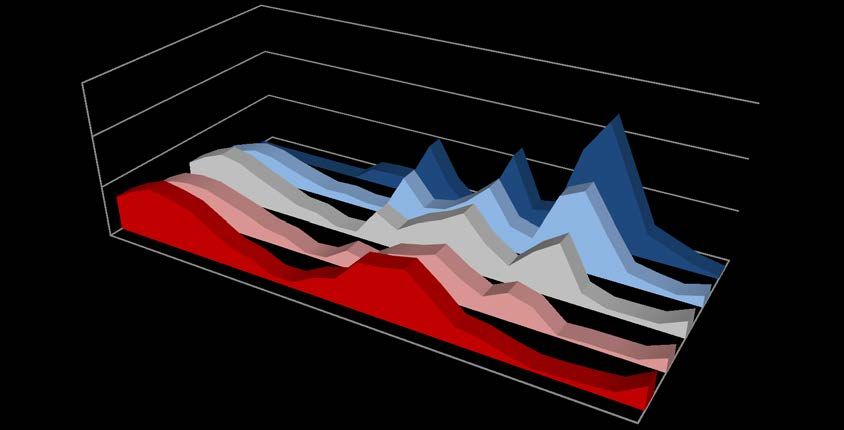
rived from the so-called Grid Development Plan (NEP). 5 This plan is drafted on a yearly basis by Ger-
man transmission system operators for a time horizon of 10 and 20 years. After a series of revisions
and public consultations, the NEP serves as the basis for German federal network planning legisla-
tion. In this study, we largely draw on the 2013 version of the Grid Development Plan (50Hertz et al.
2013) regarding thermal and renewable generation capacities, fuel and carbon prices (Table 3), and
specific carbon emissions. 6

 Table 3: Fuel and carbon prices

 Unit 2010 2020 2030
 Oil EUR2010/t 446 543 663
 Natural gas EUR2010/MWhth 21 25 26
 Hard coal EUR2010/t coal equ. 85 80 86
 Lignite EUR2010/t MWhth 2 2 2
 CO2 certificates EUR2010/t 13 24 41

As the NEP 2013 only provides generation capacities for the years 2011, 2023, and 2033, we linearly
interpolate between these years to derive capacities for 2020 and 2030. As for nuclear power, we
use the projected phase-out schedule according to German legislation. Overall, thermal generation
capacities slightly decrease until 2030, whereas installed renewable capacities increase substantially
(Figure 1). CCGT and OCGT refer to combined or open cycle gas turbines, respectively. We also in-
clude an expensive, but unlimited backstop peak generation technology in order to ensure solvability
of the model even in cases of extreme vehicle charging patterns.

5
 Netzentwicklungsplan (NEP) in German.
6
 More precisely, we draw on the medium projections called “B 2023” and “B 2033”, which are deemed to be
the most likely scenarios. We also draw on the 2012 and 2014 versions of the NEP in some instances, e.g., re-
garding 2010 generation capacities as well as 2012 offshore wind capacities (50Hertz et al. 2012, 50Hertz et al.
2014).

 7
300

 Bio
 250
 Hydro
 PV
 200 Wind offshore
 Wind onshore
 Pumped hydro strorage
 GW

 150
 Other thermal
 Oil
 100
 CCGT and OCGT
 Hard coal
 50
 Lignite
 Nuclear
 0
 2010 2020 2030

 Figure 1: Installed net generation capacities

Hourly availability factors of onshore wind and PV are derived from publicly available feed-in data of
the year 2010 provided by German TSOs. We project hourly maximum generation levels of these
technologies for the years 2020 and 2030 by linearly scaling up to the generation capacities of the
respective year. As for offshore wind, feed-in data is available for selected projects in the North Sea
only. We derive hourly availability factors from publicly available 2012 feed-in data provided by the
transmission system operator TenneT.

Hourly power demand is assumed not to change compared to 2010 levels. We assume a total yearly
net consumption of 560.8 TWh, including grid losses, with a maximum hourly peak load of 91.9 GW.
As regards other techno-economic parameters such as efficiency of thermal generators, start-up
costs, and minimum off-times, we draw on DIW Berlin’s power plant database, Egerer et al. (2014),
and own research.

All exogenous model parameters related to electric vehicles are provided by Kasten and Hacker
(2014). 7 The assumed fleets of electric vehicles of the years 2020 and 2030 in the two scenarios BAU
and EM+ imply aggregate hourly power consumption and maximum charging profiles of 28 vehicle
categories, of which 16 relate to pure battery-electric vehicles (BEV) and 12 to plug-in hybrid electric
vehicles (PHEV) or range extender electric vehicles (REEV). Vehicles differ with respect to both their
battery capacity and their typical charging power. All vehicles may be charged with a net power of
10.45 kW in some hours of the year, as these are assumed to be connected to (semi-)public “medium
power charging stations” occasionally. Table 4 provides an overview of EV-related parameters. The

7
 There is one exception: the parameter ℎ is set exogenously by us, depending on the scenario
run.

 8
cumulative battery capacity in the 2030 is in the same order of magnitude as the power storage ca-
pacity of existing German pumped hydro storage facilities. The table also includes an indicative yearly
average value of hourly recharging capacities which reflects different assumptions on hourly connec-
tivity to charging stations and different charging power ratings.

 Table 4: Exogenous parameters related to electric vehicles

 2020 2030
 +
 BAU EM BAU EM+
 Number of vehicles (million)
 BEV 0.1 0.1 0.9 1.0
 PHEV/REEV 0.3 0.4 2.9 3.7
 Overall 0.4 0.5 3.7 4.8
 Cumulative battery capacity (GWh)
 BEV 2.4 2.8 21.7 25.2
 PHEV/REEV 3.0 3.9 27.6 35.9
 Overall 5.4 6.7 49.2 61.1
 Cumulative average hourly charging capacity (GW)
 BEV 0.3 0.3 2.9 3.1
 PHEV/REEV 0.7 0.8 8.7 10.3
 Overall 1.0 1.1 11.6 13.3

Just like wholesale power demand, power consumption by electric vehicles is assumed to be perfect-
ly price-inelastic. As regards plug-in hybrid electric vehicles, we ensure a preference for electric driv-
ing mode by including a penalty on conventional fuel use in the objective function.

4 Results
In the following, we compare the model outcomes with respect to EV charging patterns, dispatch of
thermal and renewable generators, renewable curtailment, charging costs, and CO2 emissions.

4.1 Charging of electric vehicles
The yearly power consumption of electric vehicles in the different scenarios is generally small com-
pared to overall power demand (Table 5). In 2020, the EV fleet consumes 0.7 TWh in the BAU scenar-
ios and around 0.9 TWh in the EM+ scenarios. These values correspond to only around 0.1% of total
power consumption, or 0.2%, respectively. In terms of overall energy consumption, the impact of
around half a million EVs may thus be considered negligible in Germany. In 2030, EV-related power
consumption gets more significant with up to 7.1 TWh in BAU and nearly 9.0 TWh in EM+, which cor-
responds to around 1.3% of total power consumption, or 1.6%, respectively. In the user-driven charg-
ing modes power consumption is generally slightly lower compared to cost-driven charging because
the electric shares of PHEV and REEV are slightly lower. These electric utility factors are around 55%
in the 2020 scenarios, and between 60% (user-driven) and 64% (cost-driven) in the 2030 scenarios.
This is in line with other model-based analyses. Kelly et al. (2012) estimate a utility factor of around
67% based on data from 170,000 vehicle’s driving patterns in the U.S. The slightly higher value is

 9
probably caused by the assumption of larger batteries in future PHEV. Weiller (2011) also determines
utility factors for U.S. PHEV between 50% and 70%, depending on the battery size and car usage.

 Table 5: Power consumption of electric vehicles

 EV scenario Charging mode Generation capacities EV consump- Share of total
 tion (TWh) load (%)
 2020 2030 2020 2030
 User-driven 0.70 6.92 0.12 1.22
 BAU Baseline
 Cost-driven 0.70 7.10 0.12 1.25
 User-driven 0.88 8.59 0.16 1.51
 75% fast charge 8.90 1.56
 50% fast charge Baseline 8.95 1.57
 25% fast charge 8.95 1.57
 Cost-driven 0.88 8.95 0.16 1.57
 EM+ 100% Wind 8.54 1.50
 User-driven 50% Wind/PV 8.55 1.50
 100% PV 8.59 1.51
 RE+
 100% Wind 8.95 1.57
 Cost-driven 50% Wind/PV 8.95 1.57
 100% PV 8.95 1.57

While overall power consumption of the assumed EV fleets is rather small compared to overall power
demand, hourly charging loads vary significantly over time and sometimes become rather high. This
is especially visible in the case of user-driven charging, where charging takes place without consider-
ation of current power system conditions. Here, EVs are charged as fast as possible given the re-
strictions of the grid connection. 8 Figure 2 exemplarily shows the average charging power over 24
hours for the 2030 EM+ scenario (with baseline generation capacity assumptions). User-driven charg-
ing results, on average, in three distinct daily load peaks. These occur directly after typical driving
activities. Almost no charging takes place at night, as EVs are fully charged several hours after the last
drive. In contrast, the cost-driven charging mode allows to charge EVs during hours of high PV availa-
bility, and to shift charging activities into the night, when other electricity demand is low. Overall, the
average charging profile is much flatter in the cost-driven mode compared to the user-driven one.

8
 We do not consider possible restrictions related to bottlenecks in both the transmission and the distribution
grids, which may pose barriers to both the fully user-driven and the fully cost-driven charging modes.

 10
6

 GW
 5

 4

 3

 2

 1

 0
 0 1 2 3 4 5 6 7 8 9 10 11 12 13 14 15 16 17 18 19 20 21 22 23

 2030 EM+ user-driven 2030 EM+ cost-driven

 Figure 2: Average EV charging power over 24 hours (2030, EM+)

While Figure 2 only shows average charging power under the two extreme modes, Figure 3 provides
additional information for the cases with intermediate charging modes, in which at least 25%, 50%,
or 75% of the vehicles’ battery capacities have to be recharged as quickly as possible after the vehi-
cles are connected to the grid. Even a slight relaxation of the fully user-driven mode, i.e., reducing
 ℎ from 1 to 0.75, results in a substantially smoothed load profile, while presuma-
bly only slightly reducing the users’ utility. The maximum average charging load peak in the evening
hours accordingly decreases from 4.9 to 3.1 GW. Reducing ℎ further to 0.5 entails
additional smoothing, with a corresponding reduction of the evening load peak to 2.1 GW.

 6

 4

 2

 0
 1
 3 1
 5
 7 0.75
 9
 11 0.5
 13
 15 0.25
 17
 19 0
 21
 23

Figure 3: Average EV charging power over 24 hours for intermediate charging modes (2030, EM+)

 11
From a power system perspective, the impact of electric vehicles on the load duration curve, in par-
ticular on the system’s peak load, may be more relevant than average charging levels. For the 2030
EM+ scenarios, Figure 4 shows the load duration curve of the case without electric vehicles (right
vertical axis) as well as additional loads imposed on the system’s load duration curve induced by EVs
under different charging modes (left vertical axis). The latter are derived as follows: first, we establish
the load duration curves of all scenarios by sorting hourly loads in descending order. Then, hourly
differences between these sorted load duration cures are calculated. That is, the differences shown
in Figure 4 refer to load deviations between hours with the same position in the load duration curve,
but not necessarily between the same hours, i.e., the index will typically differ.

 5,0 100
 4,5 90
 4,0 80
 3,5 70
 cost-driven
 3,0 60
 25% fast charge
 GW

 GW
 2,5 50
 50% fast charge
 2,0 40
 75% fast charge
 1,5 30
 user-driven
 1,0 20 No EVs (right axis)
 0,5 10
 0,0 0
 1 1001 2001 3001 4001 5001 6001 7001 8001
 hours

 Figure 4: Impacts of EVs on the load duration curve under different charging modes (2030, EM+)

Figure 4 shows that user-driven charging generally makes the load duration curve of the system
steeper, as additional power is mainly required on the left-hand side. That is, user-driven charging
increases the system load during hours in which demand is already high. On the very left-hand side,
the peak load in the fully user-driven mode increases by around 3.6 GW, compared to only 1.5 GW in
the purely cost-driven mode. In contrast, cost-driven charging largely occurs on the right-hand-side
of the load duration curve, which implies a better utilization of generation capacities plants during
off-peak hours. We again find a strong effect of even slightly deviating from the fully user-driven
mode: reducing ℎ from 1 to 0.75, i.e., requiring only 75% of the battery capacity to
be charged instantaneously instead of 100%, results in substantial smoothing of the residual load
curve. If this parameter is further reduced to 50%, the load duration curve closely resembles the one
of the fully cost-driven charging mode.

It should be noted that the backstop peak technology is required in the 2030 scenarios under fully
user-driven charging in order to solve the model. That is, the generation capacities depicted in Figure

 12
1 do not suffice to serve overall power demand during peak charging hours. The NEP generation ca-
pacities are exceeded by around 220 MW in the peak hour of the user-driven 2030 BAU scenario, and
by around 360 MW in the respective EM+ scenario. In other words, user-driven charging would raise
severe concerns with respect to generation adequacy and may ultimately jeopardize the stability of
the power system.

4.2 Power plant dispatch
The differences in hourly EV charging patterns discussed above are reflected in a changed dispatch of
the power plant fleet. 9 While EV-related power requirements in the user-driven case mainly have to
be provided during daytime, cost-driven charging allows, for example, utilizing idle generation capac-
ities in off-peak hours. Comparing dispatch in the 2020 EM+ scenario to the one in the case without
any electric vehicles in the same year, we find that the introduction of electric vehicles under cost-
driven charging mostly increases the utilization of lignite plants, which have the lowest marginal
costs of all thermal technologies (Figure 5). Generation from mid-load hard coal plants also increases
substantially. These changes in dispatch are enabled by the charging mode, which allows shifting
charging to off-peak hours in which lignite and hard-coal plants are under-utilized. Under user-driven
charging, power generation from lignite cannot be increased that much, as charging occurs in periods
in which these plants are largely producing at full capacity, anyway. Instead, generation from hard
coal grows even more than in the cost-driven case. In addition, user-driven charging increases the
utilization of–comparatively expensive–gas-fired plants, as these are the cheapest idle capacities in
many recharging periods, e.g., during weekday evenings. The utilization of pumped hydro storage
decreases slightly under cost-driven charging, as optimized charging of electric vehicles diminishes
arbitrage opportunities of storage facilities. In contrast, storage use increases slightly under user-
driven charging because of increased arbitrage opportunities between peak and off-peak hours.

9 +
 Regarding power plant dispatch, we only present results for the EM scenarios of 2020 and 2030 as well as
 +
2030 RE . The respective dispatch results in the BAU scenarios are very similar, but less pronounced than the
 + +
ones of the EM and RE runs.

 13
Pumped hydro
 Biomass
 Wind and PV
 Other thermal
 Oil
 OCGT
 CCGT
 Hard coal
 Lignite
 Nuclear

 -0,1 0,0 0,1 0,2 0,3 0,4 0,5
 TWh

 2020 EM+ user-driven 2020 EM+ cost-driven

 Figure 5: Dispatch changes relative to scenario without EV (2020, EM+)

Figure 6 shows respective changes in dispatch outcomes for the 2030 EM+ scenario. Compared to the
2020 results presented above, the introduction of electric vehicles has a much more pronounced
effect in 2030, as the overall number of electric vehicles is much higher. While the direction of dis-
patch changes is largely the same as in 2020, there is a slight shift from lignite to gas: under cost-
driven charging, the relative increase in the utilization of lignite plants is less pronounced compared
to 2020, whereas the utilization of combined cycle gas turbines (CCGT) is higher. Under user-driven
charging, this effect–which can be explained by an exogenous decrease of lignite plants and a corre-
sponding increase of gas-fired generation capacities (cf. Figure 1)–is even more pronounced, such
that most of the additional power generation comes from CCGT plants. Worth mentioning, the addi-
tional flexibility brought to the system by cost-driven charging also enables additional integration of
energy from renewable sources, i.e., onshore and offshore wind as well as PV. Correspondingly,
pumped storage, which is another potential source of flexibility, is used less in the cost-driven case. It
can also be seen that reducing the fast charging requirement from 100% to 75% strongly alters the
dispatch into the direction of the cost-driven outcomes. Reducing the requirement to 50% entails
largely the same dispatch as the fully cost-driven charging mode.

 14
Pumped hydro
 2030 EM+ user-driven
 Biomass 2030 EM+ 75% fast charge

 Wind and PV 2030 EM+ 50% fast charge
 2030 EM+ 25% fast charge
 Other thermal
 2030 EM+ cost-driven

 Oil

 OCGT

 CCGT

 Hard coal

 Lignite

 -1,0 0,0 1,0 2,0 3,0 4,0
 TWh

 Figure 6: Dispatch changes relative to scenario without EV (2030, EM+)

In the cases presented so far, we have assumed that the power plant fleets of the years 2020 or 2030
do not change between the cases with and without electric vehicles. While this assumption proves to
be unproblematic with respect to overall generation capacities–at least in the cost-driven charging
mode–we are interested in how results change if the power plant fleet is adjusted to the introduction
of electric mobility. While there are many thinkable changes to the generation portfolio 10, we are
particularly interested in cases in which the introduction of electric vehicles goes along with a corre-
sponding increase in renewable energy generation. In fact, German policy makers have directly
linked the introduction of electric vehicles to the utilization of renewable power (Bundesregierung
2011). Yet results presented so far have shown that the additional energy used to charge EVs is main-
ly provided by conventional power plants, and particularly by emission-intensive lignite plants in the
cost-driven charging mode.

We thus conduct additional “Renewable Energy+“ (RE+) model runs based on the 2030 EM+ scenario.
We add onshore wind and/or photovoltaics capacities to such an extent that their potential yearly
feed-in exactly matches the amount of energy required to charge EVs. We distinguish three cases in
which this power is generated either fully from onshore wind or PV, or 50% from onshore wind and
50% from PV (Table 6). 11 Note that the required PV capacities are much larger compared to onshore
wind because of PV’s lower average availability. In the cost-driven charging mode, capacities are

10
 For example, additional open cycle gas turbines may be beneficial under user-driven charging, while addi-
tional baseload plants may constitute a least-cost option under cost-driven charging. Note that we do not de-
termine cost-minimal generation capacity expansion endogenously, as we use a dispatch model in which gen-
eration capacities enter as exogenous parameters.
11
 Onshore wind and PV obviously incur different capital costs. We do not aim to determine a cost-minimizing
portfolio; rather, we are interested in the effects of different technology choices on dispatch outcomes.

 15
slightly higher than in the user-driven mode, as the overall power consumption of PHEV and REEV is
higher.

 Table 6: Additional generation capacities in RE+ scenarios (in MW)

 Charging mode 100% Wind 100% PV 50% Wind/PV
 Wind PV
 User-driven 6,176 13,235 3,088 6,617
 Cost-driven 6,438 13,795 3,219 6,897

We compare the outcomes of the RE+ cases to the 2030 scenario without EVs and without additional
renewables. 12 This may be interpreted as a setting in which the deployment of renewables is strictly
linked to an additional deployment of renewables, which would not have occurred without the intro-
duction of electric mobility. Figure 7 shows the dispatch changes induced by electric vehicles and
additional renewables for the three cases 100% Wind, 100% PV, and 50% Wind/PV each. Not surpris-
ingly, the additional energy is predominantly provided by the exogenously added renewable capaci-
ties in all cases. Under user-driven charging, lignite plants are used less, while gas-fired plants and
pumped hydro stations are increasingly utilized. This can be explained by increasing flexibility re-
quirements in the power system induced by both additional (inflexible) EV charging and fluctuating
renewables.

In contrast, dispatch of thermal generators changes substantially under cost-driven charging. Power
generation from lignite increases compared to the case without electric vehicles, whereas gas-fired
plants and pumped hydro facilities are used less. This is because the system-optimized EV fleet brings
enough flexibility to the power system to replace pumped hydro and gas-fired plants and at the same
time increase generation from rather inflexible lignite plants at the same time. This flexibility also
allows slightly increasing the overall utilization of renewables as compared to the user-drive mode.

12 + +
 An additional comparison of RE results to the respective 2030 EM outcomes allows separating the effects of
introducing EV and additional renewable capacities. A comparison of the user-driven cases shows that addi-
tional renewables mainly substitute hard coal and CCGT, while lignite is substituted to a minor extent. Compar-
 + +
ing RE to EM under cost-driven charging leads to similar results, yet the substitution effect is slightly stronger
as cost-driven charging allows increasing the integration of fluctuating renewables, in particularly PV.

 16
Pumped hydro

 Biomass

 Wind and PV

 Other thermal
 2030 RE+ cost-driven - 100% Wind
 Oil
 2030 RE+ cost-driven - 100% PV

 OCGT 2030 RE+ cost-driven - 50% Wind/PV
 2030 RE+ user-driven - 100% Wind
 CCGT 2030 RE+ user-driven - 100% PV
 2030 RE+ user-driven - 50% Wind/PV
 Hard coal

 Lignite

 -2 0 2 4 6 8 10
 TWh

 Figure 7: Dispatch changes relative to scenario without EV (2030, RE+)

Finally, we compare the cases with respect to the integration of fluctuating renewables. It has often
been argued that future electric vehicle fleets may help to foster the system integration of fluctuat-
ing renewables (compare Hota et al. 2014). Our model results show that the potential of EVs to re-
duce renewable curtailment is rather low under user-driven charging, but sizeable in case of cost-
driven charging (Figure 8). 13 In 2020, very little curtailment takes place, and the effect of EVs on cur-
tailment is accordingly negligible. In the 2030 EM+ scenario, about 1.3 TWh of renewable energy can-
not be used in the case without EVs, corresponding to 0.65% of the yearly power generation poten-
tial of onshore wind, offshore wind and PV. User-driven EV charging decreases this value to about
1.1 TWh (0.55%), while only 0.6 TWh of renewables have to be curtailed under cost-driven charging
(0.29%). Curtailment is generally higher in the RE+ scenarios. Among the three different portfolios of
additional renewable generators, the one with 100% PV has the lowest curtailment levels (1.9 TWh
or 0.89% in the case without electric vehicles), while curtailment is highest in the one with 100%
onshore wind (2.3 TWh or 1.07%). Cost-driven charging again results in much lower levels of renewa-
ble curtailment compared to user-driven charging.

13
 In addition, electric vehicles may indirectly foster the system integration of renewable power generators by
providing reserves and other ancillary services energies, which are increasingly required in case of growing
shares of fluctuating renewables.

 17
2,5
 TWh

 2

 1,5

 1

 0,5

 0
 No EV

 cost-driven

 No EV

 cost-driven

 No EV

 cost-driven

 No EV

 cost-driven

 No EV

 cost-driven
 user-driven

 user-driven

 user-driven

 user-driven

 user-driven
 100% Wind 100% PV 50% Wind/PV
 2020 EM+ 2030 EM+ 2030 RE+

 Figure 8: Renewable curtailment

4.3 Charging costs
The previously discussed differences in power plant dispatch are reflected by substantial differences
in the charging costs of EVs. Here, average costs of charging are calculated by comparing overall dis-
patch costs of the respective scenario to the costs of the scenario without EVs and relating the dif-
ference to the overall power consumption of EVs. 14

In the 2020 EM+ scenarios, moving from user-driven to cost-driven charging decreases average EV
loading costs from nearly 44 €/MWh to around 29 €/MWh. In the 2030 EM+ scenarios, there is a simi-
lar effect on a somewhat higher level, with average costs of 56 €/MWh in the user-driven mode and
42 €/MWh in the cost-driven mode. From a vehicle owner perspective, the cost advantages of opti-
mized charging have to be compared to real or perceived benefits of the user-driven mode, for ex-
ample, not handing over control of charging to a third party, or the flexibility to use the car sooner
than previously planned. Interestingly, requiring only 75% of the battery to be charged as soon as
possible instead of 100% already reduces average loading costs in the 2030 EM+ scenarios from 56
€/MWh to 49 €/MWh, i.e., roughly the average of the outcomes for fully cost-driven and fully user-
driven charging. Reducing ℎ to 50% further reduces costs to 45 €/MWh.

When calculating the charging costs of the 2030 RE+ cases, we proceed as described above, but also
take into account the investments required for the additional wind and PV capacities. To do so, we
calculate investment annuities, drawing on the cost projections of Schröder et al. (2013), an econom-

14
 Alternatively, hourly power prices–i.e., the marginal values of equation (14) in the Appendix–in the periods
of vehicle loading could be used. Prices in unit commitment models, however, do not include start-up costs.

 18
ic lifetime of 20 years and an interest rate of 4%. It should be noted that this approach attributes the
dispatch cost changes of introducing both additional renewables and electric vehicles fully to EV
charging costs. Average EV charging costs in the cost-driven mode are around 58 €/MWh for the
100% Wind case (61 €/MWh for 100% PV, and 59 €/MWh for 50% Wind/PV). The difference to aver-
age charging costs in the EM+ scenario may be interpreted as the additional cost of linking EVs to
renewables. In the user-driven mode, average charging costs are much higher with 93 €/MWh for the
100% Wind case (120 €/MWh for 100% PV, and 118 €/MWh for 50% Wind/PV). Accordingly, linking
the introduction of electric vehicles to an according additional system integration of renewables be-
comes much cheaper if the vehicles are charged in a cost-optimized way.

4.4 CO2 emissions
The changes in dispatch, which are discussed in detail in section 4.2, are reflected by changes in CO2
emissions. 15 As shown above, the introduction of electric mobility may increase the utilization of
both base-load capacities such as lignite and fluctuating renewables. While the first tends to increase
CO2 emissions, the latter has an opposite effect. Both effects overlap. The net effect on emissions is
shown in Figure 9, which features specific emissions of both overall power consumption and EV’s
charging electricity. The latter are calculated as the difference of overall CO2 emissions between the
respective case and the scenario without electric vehicles, related to the overall power consumption
of EVs.

 900
 800
 700
 600
 500
 g/kWh

 400
 300
 200
 100
 0
 -100
 cost-driven

 cost-driven

 cost-driven

 cost-driven

 cost-driven

 cost-driven

 cost-driven
 user-driven

 user-driven

 user-driven

 user-driven

 user-driven

 user-driven

 user-driven

 No EV BAU EM+ BAU EM+ 100% Wind 100% PV 50%
 Wind/PV
 2010 2020 2030 2030 RE+

 Overall power consumption EV charging electricity

 Figure 9: Specific CO2 emissions

15
 It should be noted that the dispatch model not only considers CO2 emissions related to the actual generation
of power, but also to the start-up of thermal power plants.

 19
Due to ongoing deployment of renewable generators, specific CO2 emissions of the overall power
consumption change from around 490 g/kWh in 2010 16 to around 400 g/kWh in 2020, less than
330 g/kWh in the 2030 BAU and EM+ scenarios, and around 320 g/kWh in the 2030 RE+ scenarios. In
the BAU and EM+ scenarios of both 2020 and 2030, specific emissions of the EV charging electricity
are substantially larger than average specific emissions, as a sizeable fraction of the charging electric-
ity is generated from emission-intensive energy sources like lignite and hard-coal. 17 In terms of CO2
emissions, the slight improvements in renewable integration related to EVs are by far outweighed by
the increases in power generation from conventional plants. Only in the 2030 RE+ scenarios, in which
the introduction of electric vehicles goes along with additional renewable generation capacities, spe-
cific emissions of the charging electricity are well below the system-wide average, and even turn
negative in some cases. The latter can be interpreted such that the combined introduction of EVs and
additional renewables not only results in emission-neutral electric mobility, but the additional de-
mand of EVs also triggers a slightly better integration of renewables in the power system at large.
Note that we compare the RE+ scenarios to the same reference scenario as the 2030 EM+ runs, i.e., a
2030 scenario without EVs and without additional renewable generation capacities. The system-wide
emission effect of additional renewables is thus fully attributed to electric vehicles, even if EVs are
not fully charged with renewable power during the actual hours of charging.

Among the two different charging strategies, the cost-driven mode always leads to higher emissions
compared to the user-driven mode, as the first allows for switching some charging activities into
hours in which lignite plants are under-utilized, whereas the latter forces charging to happen mostly
in hours in which lignite and hard-coal plants are already fully utilized. Interestingly, this outcome
contrast the findings of Göransson et al. (2010), which show for a Danish case study that user-driven
charging may increase system-wide CO2 emissions, whereas cost-driven charging may result in an
absolute decrease of emissions. These differences can be explained by different power plant fleets in
the two case studies: The Danish system has low capacities of emission-intensive generators and very
high shares of wind, with accordingly high levels of curtailment. In contrast, our German application
features much higher capacities of emission-intensive generators as well as lower shares of wind
power. Accordingly, the increase in power system flexibility related to cost-driven EV charging is pre-
dominantly used for reducing renewable curtailment in the Danish case and for increasing the utiliza-
tion of lignite and hard-coal plants in Germany. For the German case, this may change in the future if
emission-intensive plants leave the system and renewable curtailment gains importance.

5 Discussion of limitations
We briefly discuss some of the model limitations and their likely impacts on results. First, the future
development of exogenous model parameters is generally uncertain. This refers, in particular, to the
development of the German power plant fleet and electricity demand, as well as cost parameters.
Because of such uncertainty, we have decided to largely draw on the assumptions of a well-

16
 According to our model results. The officially reported CO2 intensity for 2010 is slightly higher. Yet in this
context, only the relation between different scenarios is relevant, and not so much absolute emission levels.
17
 This finding relativizes a qualitative argument brought forward by Schill (2010), according to which future
improvements in CO2 emissions of the overall power system should have a positive influence on the emission
balance of EVs.

 20
established scenario (50Hertz et al. 2013). In this way, meaningful comparisons to other studies
which lean on the same scenario are possible. On the downside, the power plant fleet is necessarily
not optimized for the integration of electric vehicles. This shortcoming, however, should not have a
large impact on results, as overall power consumption of electric vehicles is very small compared to
power demand at large. In general, the effect of different assumptions on, for example, the power
plant fleet, CO2 prices, or diverging EV profiles, could be assessed by carrying out sensitivity analyses.
As regards our projections of future power generation from fluctuating renewables, drawing on feed-
in data of other years than 2010 may lead to slightly different results with regard to renewable cur-
tailment. What is more, calculating availability factors from historic feed-in time series neglects po-
tential smoothing effects related to future changes in generator design or changes in the geograph-
ical distribution. This may result in exaggerated assessments of both fluctuation and surplus genera-
tion, as discussed by Schill (2014).

Next, our dispatch model assumes perfectly uncongested transmission and distribution networks.
This assumption appears to be reasonable with respect to the transmission grid, as the NEP foresees
substantial network expansion. Yet on the distribution level, a massive deployment of electric vehi-
cles may lead to local congestion. Such local effects can hardly be considered in a power system
model as the one used here. It is reasonable to assume that congestion in distribution grids may put
additional constraints on the charging patterns of electric vehicles. While this effect should in general
be relevant for both the user-driven and the cost-driven charging mode, distribution grid bottlenecks
may be particularly significant for the user-driven mode, as charging is carried out largely in peak-
load periods in which the distribution grid is already heavily used. In case of binding distribution net-
work restrictions, both extreme modes of charging may not be fully realizable.

In addition, we abstract from interactions with neighboring countries. In the context of existing inter-
connection and European plans for further market integration in the future, this assumption appears
to be rather strong. Yet considering power exchange with neighboring countries would require a
much larger model with detailed representations of these countries’ power plant fleets. It would also
require making detailed assumption on the development of neighboring countries’ power systems as
well as on their deployment of electric vehicles. Solving a large European unit commitment model for
a full year (and various scenarios, as carried out here), would be very challenging. By treating the
German power system as an island, i.e., not considering the option of power exchange with neigh-
boring European countries, we may generally overestimate the flexibility impacts of electric vehicles
such as additional integration of lignite and renewables, as well as peak capacity problems in the
user-driven mode, as exchange with neighboring countries would entail additional flexibility which
may mitigate both peak and off-peak load situations. Our results may thus be interpreted as an up-
per boundary for the flexibility impacts of EVs on the German power system.

Next, we only consider power flows from the grid to the electric vehicle fleet (G2V) and do not con-
sider potential flows in the other direction (V2G). This assumption may be justified for the wholesale
market, as wholesale price differences likely do not suffice to make V2G economically viable with
respect to battery degradation costs (Schill 2011, Loisel et al. 2014). The provision of reserves and
other ancillary services by V2G, however, appears to be more promising (Andersson et al. 2010, Si-
oshansi and Denholm 2010, Lopes et al. 2011). Including the provision of reserves may result in high-
er levels of conventional generation, which may in turn increase renewable curtailment. This could
have important implications for the relative emission effects of user-driven and cost-driven charging
(compare the end of section 4.4). An according analysis would require extending the model to also
 21
You can also read