Pricing Methodology For Delivery Prices effective as at 1 April 2020 - Pursuant to the requirements of clause 2.4 - Alpine Energy
←
→
Page content transcription
If your browser does not render page correctly, please read the page content below
Pricing Methodology
For Delivery Prices effective as at 1 April 2020

          Pursuant to the requirements of clause 2.4
of the Electricity Information Disclosure Determination 2012
                     (consolidated in 2015)
Pricing Methodology effective 1 April 2020

                                   [Page left intentionally blank]

Alpine Energy Limited                                                Page 1 of 41
Pricing Methodology effective 1 April 2019 Contents 1. ABOUT ALPINE ENERGY ...................................................................................................... 3 2. CURRENT PRICING AND FUTURE PRICING PLANS ................................................................. 9 3. PRICING CHANGES FOR 2020/21 ....................................................................................... 14 4. HOW PRICES ARE SET........................................................................................................ 16 5. CONSUMER GROUPS ........................................................................................................ 21 6. ALLOCATING COSTS ACROSS CONSUMER GROUPS ............................................................ 24 7. ASSESSING CONSUMER IMPACTS ...................................................................................... 31 8. DO YOU HAVE ANY QUESTIONS?....................................................................................... 33 CERTIFICATION FOR THE YEAR BEGINNING 1 APRIL 2020 DISCLOSURES ....................................... 34 APPENDIX A: ALIGNMENT WITH PRICING PRINCIPLES ................................................................ 35 APPENDIX B: ALIGNMENT WITH INFORMATION DISCLOSURE REQUIREMENTS ............................ 37 APPENDIX C: LOSS FACTORS ....................................................................................................... 41 GLOSSARY ................................................................................................................................. 42 Alpine Energy Limited Page 2 of 41
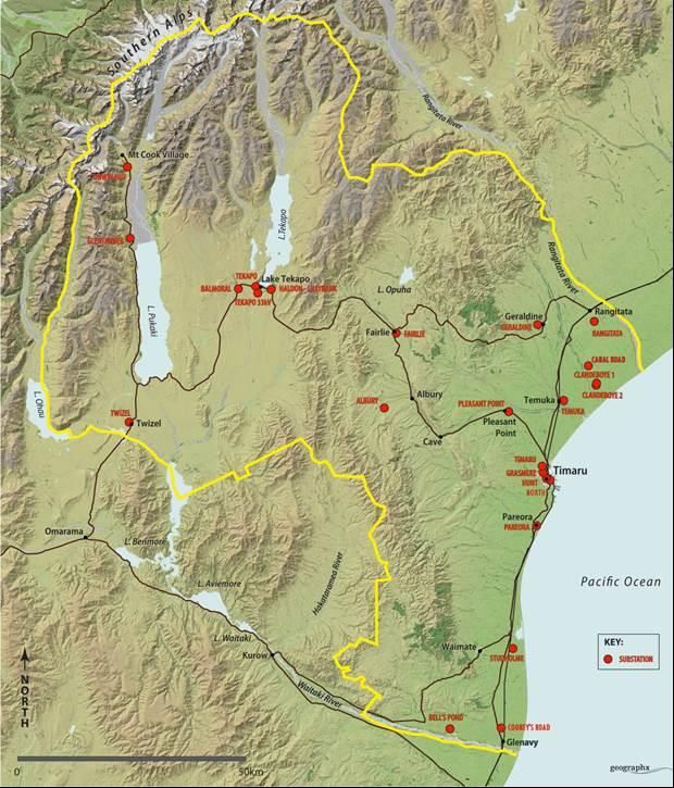
Pricing Methodology effective 1 April 2020

1. About Alpine Energy
We supply electricity to over 33,302 individual connection points throughout South
Canterbury. Our area of supply covers approximately 10,000 km2 and is located on the East
Coast of the South Island, between the Rangitata and Waitaki Rivers, and inland to Mount
Cook on the main divide.
Figure 1 Alpine Energy network, and location of the seven GXPs and 24 substations on our
network

We are 100% owned by the South Canterbury community through our shareholders.
   •   Timaru District Council (47.5%)
   •   Line Trust South Canterbury (40%)
   •   Waimate District Council (7.54%)
   •   Mackenzie District Council (4.96%).

Alpine Energy Limited                                                         Page 3 of 41
Pricing Methodology effective 1 April 2020
Since many of our consumers are also ratepayers to the local councils, they benefit directly
from our revenue, through an annual dividend payment and indirectly, through services
provided by local councils.
We want to help you understand how we set prices
This pricing methodology outlines our approach to setting electricity distribution delivery
charges to apply from 1 April 2020.
Delivery charge describes the total price we charge to transport electricity from the national
grid to consumer’s homes and businesses.
Delivery prices include:
Alpine Energy distribution charges.
Pass through charges such as rates, levies and wash-up charges that we must pay
throughout the year.
Transpower’s transmission charges.
Definitions of these charges are provided in the Glossary.
The purpose of this document is to show how our electricity pricing methodology (or
approach) sets delivery prices to recover the costs of supplying distribution services, from the
appropriate consumers, in the most efficient and fair way possible.
This section describes the role of pricing, and the network, consumer and regulatory
characteristics we consider when developing prices.
Section 2 describes our current pricing approach, and our plans to evolve pricing as
consumer preferences and technology change how our network is used.
Section 3 describes changes we made to our pricing approach and prices for 2020-21.
Section 4 describes how we set standard and non-standard prices, and distributed
generation pricing.
Section 5 describes the consumer groups paying delivery charges.
Section 6 describes how we calculate and allocate costs across consumer groups.
Section 7 describes how we assess the consumer impact of price changes.
Appendix A describes how the pricing approach aligns with the Pricing Principles published
by the Electricity Authority.
Appendix B describes how we comply with clauses 2.2.1 to 2.4.5 of the Electricity
Information Disclosure Determination 2012.
Alpine Energy Limited Page 4 of 41Pricing Methodology effective 1 April 2020
Network characteristics
The main drivers influencing electricity demand in our area relate to weather and economic
activity. Economic activity in our area of operation strongly influences the configuration of
our network.
Electricity is delivered to our network via seven grid exit points (GXPs) with Transpower and
one embedded generator at the Opuha dam. The total energy consumed in 2018/19 was 817
GWh. Energy consumed varies from year to year depending on wet or dry irrigation seasons,
and severe or mild winters. The coincident peak demand (CPD) is presently 140MW. Growth
in CPD has been approximately 2.49% per year over the last 18 years.
More detail on the network characteristics for the seven supply areas is outlined in Table 1.
Table 1 Network characteristics for the seven supply areas (GXPs)
Over the last decade, we have been through a major economic growth phase in South
Canterbury mainly due to dairy conversions, irrigation schemes and dairy processing.
The demand for new connections during 2019 was constant even after the improvement in
milk pay-outs from the dairy companies, and a reduction in irrigation connections. Growth in
demand is generally driven by irrigation, industrial, commercial, and domestic subdivision
connections and extensions. Lately we have had much activity in the area of subdivisions and
industrial development. With the government withdrawing support for the Hunter Downs
irrigation scheme, we have experienced a reduction in the number of on farm irrigation
developments
Table 2 Main load type and forecast capacity adequacy for main supply areas (GXPs) summarises
the main load type and forecast capacity adequacy for each supply area.
Table 2 Main load type and forecast capacity adequacy for main supply areas (GXPs)
Load type and forecast capacity adequacy
Location / GXP
Albury Small townships, sheep & beef farming, some
dairying. Adequate capacity to meet a small growing
demand
Bells Pond Dairy processing and on farm dairying irrigation.
Adequate capacity to meet the growing demand
Studholme Sheep and beef farming, some dairying.
Tekapo Twizel and Tekapo townships experiencing significant
Twizel growth; dairy conversions and irrigation
Alpine Energy Limited Page 5 of 41Pricing Methodology effective 1 April 2020
developments slowing due to land use/discharge
requirements. Major upgrades expected in next 5
years
Temuka Temuka and Geraldine townships, and dairying
irrigation. Adequate capacity to meet a small growing
demand. Major replacements and upgrades will be
required if there is an increase in Fonterra’s dairy
factory demand requirements
Timaru Timaru – residential, commercial and light industrial.
Upgrading supply to Washdyke industrial area.
Adequate capacity to meet growing demand
Source: Alpine Energy Limited, 2019 Asset Management Plan
More detail on our network characteristics is in our Asset Management Plan, available at
https://www.alpineenergy.co.nz/__data/assets/pdf_file/0018/8541/ALPINE-ENERGY-AMP-
2019.pdf.
The network is experiencing congestion in some areas from distributed generation exporting
into the network. In 2017 we surpassed 1 MW in PV solar installations on our network and
even though 2017 saw a reduction in the number of installations, applications picked up in
2018 with a record number of installations and overall capacity. We have also connected our
second bio gas distributed generator on our network and expect this type of installation to
increase due to the large number of dairy farms across our network and the increasing
pressure on farmers to reduce carbon emissions.
The list of export congestion areas is available on our website at:
https://www.alpineenergy.co.nz/customers/generating-electricity/export-congestion-areas.
If export congestion causes operational issues, we may interrupt the connection of any
distributed generation to the distribution network, or curtail either the operation or output
of distributed generation, or both, and may temporarily disconnect the distributed generation
from the distribution network.
Consumer characteristics
With our network covering an area between the Rangitata and Waitaki rivers, from the coast
all the way to Mt Cook, we supply the communities of Timaru, Temuka, Waimate, and
MacKenzie basin and surrounding areas. There are currently 19 retailers operating on our
network. Almost 42% of our consumers are served by one retailer. Except for six large
consumers that we directly invoice for electricity line charges, our line charges are passed to
consumers along with transmission charges and energy supply charges by the electricity
retailers. Table 3 shows the number of consumers (ICPs) in each supply area.
Alpine Energy Limited Page 6 of 41Pricing Methodology effective 1 April 2020
Table 3 ICP count and percentage of total by region at 31 March 2019
Location ICP Count %
Timaru 16,037 48%
Waimate 3,706 11%
Temuka 3,489 10%
Geraldine 3,049 9%
Twizel 1,635 5%
Pleasant Point 1,269 4%
Fairlie 1,183 4%
Lake Tekapo 827 2%
Pareora 473 1%
Orari 302 1%
Glenavy 264 1%
St Andrews 235 1%
Winchester 224 1%
Cave 208 1%
Albury 182 1%
Makikihi 112 0%
Mount Cook 107 0%
Grand Total 33,302 100%
The Timaru GXP constitutes almost half of the Alpine Network connection points and
consumption which is primarily residential, commercial and small industrial customers. Figure
2 shows the load profile for Timaru.
Figure 2 Daily maximum and minimum demand for Timaru April 2018 to March 2019
Winter peak loading occurs mainly at Timaru and Tekapo GXPs, although other areas, like
Fairlie and Geraldine, also have significant demand for load during the winter months. Winter
load demand may rise due to more regulation around air quality and particulate matter,
restricting the use of fires for heating and placing greater demand on the network to service
other forms of heating, such as heat pumps and other conventional electric heating.
The increase in tourism and subdivisions in Tekapo and Twizel is now also a driver we use in
our forecasting models.
Alpine Energy Limited Page 7 of 41Pricing Methodology effective 1 April 2020
The peak demand in the dairy industry occurs in spring and extends into early summer. Load
requirements are for processing, on-farm milking, heating and cooling as well as irrigation.
Reliability of supply is therefore very important in this industry. As a result, most shutdowns
for maintenance or network upgrade activities have to be planned for the dairy ‘off’ season.
At an individual farm level, operations are intensifying due to increasing cooling and holding
standards. There is greater use of irrigation and new technologies. There is an increasing
requirement for higher reliability of supply and better quality of supply than was previously
the case. This growth has consumed most of our spare network capacity, with major new
builds in areas where no infrastructure existed.
There has been significant growth in dairy farming and processing, bringing an increased
demand from irrigation. Irrigation load is the main cause of summer peak loading at all the
GXPs except Timaru, Tekapo, and Twizel although the increase in irrigation is tempered by
local environmental restrictions on water use, land intensification, and nitrogen discharge
limits.
Our large industrial and commercial consumers are mainly located in Timaru and more
specifically around the port, Redruth and Washdyke areas.
Regulatory characteristics
Our pricing approach is influenced by a range of regulatory requirements, including
obligations imposed by the Commerce Commission and Electricity Authority, and through the
Electricity (Low Fixed Charge Tariff for Domestic Consumers) Regulations 2004.
The main implications are:
We are required to set prices to recover no more than the revenue allowed by the
Commerce Commission’s Electricity Distribution Services Default Price-Quality
Determination 2020, [2019] NZCC 21, 27 November 2019 (DPP Determination). Sections
5-7 of this document describe how we set prices to recover no more than the allowed
revenue.
We are required to disclose information about our pricing approach and prices by the
Commerce Commission’s Electricity Distribution Information Disclosure Determination
2012 – (consolidating all amendments as of 3 April 2018), 3 April 2018 (ID Determination).
Appendix B describes how we meet the disclosure requirement.
We are expected to set efficient and cost-reflective prices consistent with the Electricity
Authority’s Distribution Pricing Principles of February 2010. Appendix A describes how our
pricing approach aligns with the Pricing Principles.
We are required to set prices for distributed generator connecting to and using our
network according to Part 6 of the Electricity Industry Participation Code 2010 (the Code),
relating to the pricing of distributed generation. Section 4 describes how we do this.
Alpine Energy Limited Page 8 of 41Pricing Methodology effective 1 April 2020
We are required to offer primary residence consumers a low fixed charge tariff option (of
15 cents/day) by the Electricity (Low Fixed Charge Tariff Option for Domestic Consumers)
Regulations 2004 (the low fixed charge regulations). The Electricity Authority monitors and
enforces the regulations.
2. Current pricing and future pricing plans
We set delivery prices using a retail delivery approach, also referred to as an Installation
Control Point (ICP) pricing methodology. The network service is priced at the consumer’s
metering point based on the electricity consumption at that point.
Our delivery prices are set taking account of the network, consumer and regulatory
characteristics relevant to our network. As such, we recognise the importance of evolving
pricing as circumstances and characteristics change, and plan to evolve our pricing to reflect
evolving consumer expectations, technology choices, and use of the network.
Current pricing
Our delivery prices for the majority of consumers have a three-part structure, with a fixed
daily charge component, and two variable components with a volume-based charge for
daytime usage (7am to 11pm) and a volume-based charge for night-time usage (11pm to
7am).
Delivery prices for connections with time-of-use metering, and capacity greater than 15kVA
have a four-part structure, with an additional fixed kw/day capacity charge component.
An overview of the current price structure and price components for each consumer groups
is provided in Table 4. More detail on each consumer group is provided in section 6.
Table 4 Overview of current price structure and price components for each consumer group
2020/21
Consumer Forecast Description Fixed Fixed Variable Variable
group # ICPs component component component component
$/day $/kW/day $/kwh - day $/kwh -
night
LOWHCA 1863 Households using $0.15 $0.12 $0.08Pricing Methodology effective 1 April 2020
Consumer Forecast Description Fixed Fixed Variable Variable
group # ICPs component component component component
metering, controlled, high
cost area
015LCA 12415 Households and small $1.29 $0.07 $0.03
commercial, 0-15kVA, <
60amp fuse, no TOU
metering, controlled, low
cost area
015UHCA 34 Households and small $1.93 $0.07 $0.03
commercial, 0-15kVA, <
60amp fuse, no TOU
metering, uncontrolled,
high cost area
015ULCA 42 Households and small $1.77 $0.07 $0.03
commercial, 0-15kVA, <
60amp fuse, no TOU
metering, uncontrolled,
low cost area
360HCA 542 Households and $6.07 $0.07 $0.03
Commercial, 3 phase, 60
amp connection, no TOU
metering, controlled, high
cost area
360LCA 768 Households and $4.38 $0.07 $0.03
Commercial, 3 phase, 60
amp connection, no TOU
metering, controlled, low
cost area
360UHCA 15 Households and $6.45 $0.07 $0.03
Commercial, 3 phase, 60
amp connection, no TOU
metering, uncontrolled,
high cost area
360ULCA 16 Households and $4.88 $0.07 $0.03
Commercial, 3 phase, 60
amp connection, no TOU
metering, uncontrolled,
low cost area
ASSHCA 1356 Commercial and Industrial, $1.98 $0.10 $0.07 $0.03
capacity > 15kVA, high cost
area
ASSLCA 417 Commercial and Industrial, $1.35 $0.09 $0.07 $0.03
capacity > 15kVA, low cost
area
TOU400HCA 38 Commercial and Industrial $1.39 $0.42 $0.02 $0.01
connected to LV network,
TOU metering, high cost
area
TOU400LCA 102 Commercial and Industrial $1.10 $0.29 $0.02 $0.01
connected to LV network,
TOU metering, low cost
area
TOU11HCA 6 Commercial and Industrial, $1.15 $0.25 $0.03 $0.01
connected to 11kV
Alpine Energy Limited Page 10 of 41Pricing Methodology effective 1 April 2020
Consumer Forecast Description Fixed Fixed Variable Variable
group # ICPs component component component component
network, TOU metering,
high cost area
TOU11LCA 4 Commercial and Industrial, $ $ $ $
connected to 11kV 1.11 0.33 0.02 0.01
network, TOU metering,
low cost area
The fixed daily charge is set based on costs which are regarded as sunk costs.
The fixed charges are set to recover:
Operating Expenditure
Reliability, safety and environment
Routine and corrective maintenance and inspection
System operations and network support
Business Support
Depreciation
Revaluations
Regulatory Tax
A portion of pass through and recoverable and transmission costs
The variable day/night volume-based charges are set to recover costs of:
Operating Expenditure
Asset relocations
Asset replacement and renewal
Service Interruptions and emergencies
System Growth
Vegetation management.
A portion of pass through and recoverable and transmission costs
Alpine Energy Limited Page 11 of 41Pricing Methodology effective 1 April 2020 Evolving our pricing and prices – our strategy Our delivery prices are set to reflect our circumstances and the cost of delivering a safe, reliable electricity supply. We recognise the importance of evolving our pricing and prices as circumstances change. The overarching factor influencing our thinking of how our pricing could evolve over time is the integral role our network plays in economic development in South Canterbury. In particular, we expect ongoing changes to use of our network from dairying, irrigation, commercial and industrial development around Timaru, and tourism around Twizel and Tekapo. We also expect consumer-led uptake of new technologies, such as photovoltaics, batteries and electric vehicles, to influence use of our network, and our pricing. The number and capacity of photovoltaic distributed generators installed on our network continues to increase although erratic year on year, and in some locations can cause network operation issues due to export congestion. Figure 3 shows the rate of new distributed generators uptake since 2011. Figure 3: Number and capacity of new distributed generators However, we expect our network will continue to be the main source of getting electricity to our consumers, with distributed energy resources and enabling technology for network support rather than network replacement. We are looking to align ourselves with others in the industry doing research, trials and experimentation with new technologies at a network level, to benefit from their resources and capabilities. Finally, regulatory circumstances are influencing our pricing, with an initial 14.6% decrease from 2019/2020 to 2020/2021 and a projected 8.22% increase in allowed revenue over the 5 year period for 2020/21 to 2025/26, resulting from the Commerce Commission’s Default price path Determination in November 2019. Alpine Energy Limited Page 12 of 41
Pricing Methodology effective 1 April 2020
The following factors will also influence our pricing strategy and the direction of our future
pricing:
Outcomes and implementation of the Electricity Price Review1
Review of the Low User Fixed Charge Regulations
Guidance from the Electricity Networks Association working groups
Government policies to reduce emissions.
Pricing changes being considered
We are considering several changes to our pricing approach to reflect changing network and
consumer characteristics of our network. In brief, we are considering:
Options to address efforts to avoid charges through short-term disconnection, e.g.,
irrigators disconnecting during the winter. We think the underlying issue is the fixed
charges which consumers pay when not using irrigation pumps over the winter
months. The Alpine portion of the charge makes up the majority of a consumer’s
power bill when not being used. These charges cover fixed operating and monthly
Transpower charges.
Options to address issues associated with non-residential and other ineligible
consumers being included in the low user load group. The underlying issue is the
incentive created by the Low user regulations to avoid charges.
Options to address issues relating to the Assessed (“ASS”) price code category. The
underlying issue is only a small number of consumers in this load group have half
hourly meters, resulting in assessed demand charges being set once only when the
connection is livened.
We will be looking at these issues, and the options, during 2020. Changes, if any, would be
included in our published 2021 Pricing Methodology after the appropriate consultation with
customers.
Implementation and transition planning
We want to make sure changes to our pricing approach and pricing is implemented
effectively, and without adverse impact for consumers or customers, particularly retailers.
We will develop implementation and transition plans for changes to our pricing as part of
considering pricing issues and options.
Key to our implementation and transition planning is obtaining comprehensive half-hourly
data. We started collecting more comprehensive monthly TOU data from 1 April 2019 when
we changed billing practices. Additionally, we are currently rolling out smart meters across
our network. These meters give real-time information about consumers’ half-hour energy
1
https://www.mbie.govt.nz/assets/electricity-price-review-final-report.pdf
Alpine Energy Limited Page 13 of 41Pricing Methodology effective 1 April 2020
usage. Once the rollout is complete, real-time information on all load groups’ usage will be
available. We will require further industry collaboration in order to obtain detailed ICP
consumption data from retailers to be able to use it for pricing purposes.
Our current delivery prices do not reflect the information that will be available after the roll-
out is complete. We intend to consider how our delivery charges might be structured in a way
that anticipates and enables us to use this information when it becomes available. Changes,
if any, would be included in our published 2021 Pricing Methodology after the appropriate
consultation with customers.
Longer-term pricing direction
We expect use of our network to change as consumer preferences, economic growth and
other factors change how our network is used. We recognised our pricing approach needs to
evolve at the same time to avoid creating perverse outcomes which stop the full value of our
network, and consumer preferences, from being realised.
We will be guided by the Electricity Networks Association pricing work in determining our
longer-term pricing direction. Specific things we will consider for 2022 and the longer-term to
make sure our pricing approach evolves as network and consumer characteristics evolve are:
Introducing a power factor charge. 70 ICP’s in November 2019 had an average Power
Factor below 0.95.
Introducing EV charger charges once there is sufficient uptake of Electric Vehicles in
South Canterbury.
Introducing distributed generation charges once we are able to obtain sufficient smart
meter data for customers making use of, or importing electricity into the Alpine
Network.
Seasonal and Temporary Disconnection Fee - Charges to consumers are allocated on the basis
of a full Price Year and therefore apply for the full Price Year to recover ongoing fixed costs. If
an installation is reconnected within 12 months from the date of any disconnection the
Distributor may, at its discretion, apply a connection fee equivalent to the fixed charges
applicable during the period of disconnection. Currently we are exposed if Irrigators
disconnect for the winter.
3. Pricing changes for 2020/21
We are changing delivery prices in 2020/21 as follows:
We are reducing prices across all consumer price categories
The reasons for the changes, and the average impact on delivery prices are described below.
Our prices reflect the price path under the DPP Determination.
Alpine Energy Limited Page 14 of 41Pricing Methodology effective 1 April 2020
Changes to price levels
Our allowable distribution revenue for 2020/21 is $42.65 Million.
The median delivery price decrease from 1 April 2020 to 1 April 2021 is 16%. The decrease is
attributable to:
i) The maximum allowable revenue for distribution set at $42.65 million
ii) Transmission charges decreased to $12.57 million
iii) Pass through and recoverable costs decreasing to $3.55 million
The change in revenue for each consumer group, and average delivery price change from the
resulting changes to price levels is described in Table 5.
Table 5 Change in forecast revenue and average delivery prices between 2019/20 and 2020/21
Change in revenue Change in revenue Average delivery price
Consumer group
19/20 to 20/21 ($) 19/20 to 20/21 (%) change (%)
LOWHCA -$125,578 -9.75% -$ 130.57
LOWLCA -$806,535 -11.96% -$ 126.88
015HCA -$1,526,466 -19.59% -$ 219.51
015LCA -$3,583,095 -23.10% -$ 214.28
360HCA -$387,308 -17.48% -$ 505.96
360LCA -$684,382 -21.40% -$ 732.44
ASSHCA -$10,124,796 -45.62% -$ 2,935.22
ASSLCA -$2,016,464 -34.25% -$ 4,580.85
TOU400HCA -$628,588 -25.41% -$ 17,531.86
TOU400LCA -$2,048,838 -32.63% -$ 20,354.55
TOU11HCA -$677,938 -35.43% -$ 119,844.22
Alpine Energy Limited Page 15 of 41Pricing Methodology effective 1 April 2020
Change in revenue Change in revenue Average delivery price
Consumer group
19/20 to 20/21 ($) 19/20 to 20/21 (%) change (%)
TOU11LCA -$283,367 -26.88% -$ 69,755.79
The average change in prices is due to:
the DPP3 maximum allowable revenue set by the Commerce Commission.
A reduction in transmission charges due to a combination of a reduction in Transpower’s
recovery set by the Commerce Commission and having recovered unclaimed charges
during 2019-2020 which no longer apply in 2020-2021.
We considered the consumer impact of the delivery prices changes. Our approach to
assessing and managing consumer impact of price changes is described in section 7.
Changes to price structure
We have not changed any price structures for the current year. However, as noted in section
2, we are considering reviewing and possibly discontinuing the Assessed Load Group in future
years given that we are unable to assess the demand charges on an annual basis for non-half
hour customers.
Alpine Energy has applied the reduction in allowable revenue to the variable component of
pricing, thereby reducing the proportion of revenues recovered through variable charges, and
increasing the proportion of revenues recovered through fixed charges. The changes will
improve alignment of our pricing with our costs of supply, which are primarily fixed.
We considered the consumer impact of the delivery price structure changes. Our approach to
assessing and managing consumer impact of price changes is described in section 7.
4. How prices are set
Prices for consumers using our networks to consume electricity are set in two ways.
Standard pricing for residential and most commercial consumers supplied according to the
price categories in the standard price schedule.
Non-standard direct-billed customers.
We also set prices for distributed generators, including payments to distributed generators
providing network support services.
When setting prices, we consider the opportunity to share the value of deferring network
investment. We do this by introducing a discount to variable charges (to signal a benefit of
changing behaviour) or by directly contracting with a party supplying a network support
service.
Alpine Energy Limited Page 16 of 41Pricing Methodology effective 1 April 2020
Standard pricing
We set standard prices using the following process.
We determine consumer groups. Section 5 gives more detail.
Assign consumers (connections) to groups for allocating total costs
We calculate and allocate costs to consumer groups. Section 6 gives more detail.
Confirm the total forecast allowed revenue we can recover for the year. Forecast revenue
is determined by the Commerce Commission to reflect efficient costs of supplying
distribution services
Calculate expected costs for the year. The main component costs are operating costs
(including administration costs), capital costs (including return on investment) and
transmission costs (including ACOT)
Allocate costs to each consumer group to as closely as possible align benefit of access and
use of the distribution service and cost of supplying the distribution service
Determine price structures for each consumer group based on the relevant cost
allocations, and complying with the relevant legal requirements.
We assess consumer impacts of pricing variations. Section 7 gives more detail.
• Check the impact on consumers of pricing variations, and adjust pricing as needed.
Non-standard pricing for direct billed customers
For the period ending 31 March 2020, we had six direct billed customers (12 ICPs) connected
to our network at present. We are not expecting any new direct billed connections before 31
March 2020.
The decision to place a new connection onto a direct billed contract is made on a case by case
basis. When making this decision we take into account the:
cost of the build
number of new assets required
extent of the existing network that will be used by the new connection
capital contribution paid
ongoing costs that will be recovered through delivery prices
required security of supply.
Alpine Energy Limited Page 17 of 41Pricing Methodology effective 1 April 2020
The following methodology is used for calculating prices for directly billed customers2.
Because we enter into long term contracts with direct billed customers we are able to
negotiate outcomes which are consistent with market like arrangements.
Calculation and recovery of the cost of new assets
The capital contribution paid for new assets can reduce the ongoing delivery prices that the
customer will pay.
If a capital contribution equals the total value of the new assets allocated to the customer the
customer may not pay cost of capital or depreciation charges for these new assets. They will,
however, pay for ongoing maintenance charges for these assets through their delivery prices.
If the capital contributions do not cover the full cost of the value of new assets used by the
customer, then the remaining value of the asset (after capital contributions) will be used to
calculate cost of capital and depreciation charges. Depreciation charges are calculated on a
remaining life basis, with the age of the asset taken from the Commerce Commission’s
Optimised Deprival Value Handbook (2004).
When calculating the return on capital charges we apply the Commerce Commission’s
weighted average cost of capital for the industry, and the closing regulatory value of the new
asset (adjusted for inflation) from the previous year, using a midyear cash flow.
Capital contributions based on perceived risk of investment
We calculate the value of the capital contribution on the perceived risk of the investment.
The perceived risk is calculated using a risk algorithm which we fill out then pass to the
customer for comment. The risk algorithm calculates a percentage score which translates to
the percentage of the total investment cost that should be paid as a capital contribution. For
example, if the risk algorithm calculates risk to be 0.75 then we would require a capital
contribution of 75% of the total investment cost.
Maintenance charges payable
Maintenance charges effectively bank the cost of maintaining assets. That is, while new assets
will have little maintenance after the first year of service, the maintenance charge will cover
future replacement costs. However, the maintenance charge will not cover future costs to
upgrade capacity.
Recovering the cost of existing network assets
If the customer also requires the use of existing network assets then cost of capital charges,
depreciation, and maintenance charges apply for these assets.
2
For some direct billed customers, the pricing methodology will differ to the one described above due prior
long term contracts in place.
Alpine Energy Limited Page 18 of 41Pricing Methodology effective 1 April 2020
Allocators for recovering costs
The portion that a customer will pay for the use of existing network assets will depend on the
most relevant cost driver for that asset. For lines and cables, costs are apportioned to the
customer based on the customer’s line/cable length to the total line/cable lengths in the
network.
For sub-stations, transformers, protection, and switchgear, costs are apportioned to the asset
using the total demand or capacity3 of all users of the asset including the direct billed
customer, to the total demand or capacity of the asset type across the network. Costs are
then apportioned to the customer according to the customer’s demand or capacity to the
total demand/capacity relevant to the asset.
Recovering the future costs of grid upgrades in capacity
Please note that our costs are fixed in the short term so that a drop in consumption will have
little or no impact on our short term (annual) costs. However, a decrease in consumption over
the long term can delay or prevent upgrades in network capacity due to under-recovery of
our required revenue.
Recovery of transmission costs
Transmission costs are passed through to the customer according to the customer’s demand
to the total demand of all users of the GXP the consumer is connected to. The exception is
the interconnection charge which is charged out to the consumer at the Transpower rate per
kW of consumer demand during the regional coincident peak demand.
Difference between direct bill and standard agreement security
standards
Customers on a direct billed contract can expect one planned outage each year and an
unplanned outage of two hours every five years, plus a momentary unplanned outage every
two years4. These service standards are not available to consumers on the shared distribution
charges model. For both direct billed customers and consumers on the shared network, we
give a minimum of four working days’ notice before a planned shutdown occurs. We do not
guarantee supply or offer compensation if supply is lost to any connection.
Capital contributions
In addition to the delivery charge revenue that we receive from our consumers we also
receive capital contributions from any consumer that requires to be connected to our
network or needs upgrades to their existing connection. Costs of upgrades to an existing
connection can be shared where there are network benefits to the upgrade.
3
The use of demand or capacity will depend on the type of asset that the cost relates to.
4
Some contracted service standards will differ for older contracts.
Alpine Energy Limited Page 19 of 41Pricing Methodology effective 1 April 2020
Where the upgrade is for the sole benefit of the consumer the consumer must pay in entirety
for that upgrade.
Capital contributions cover the cost of the work carried out less rebates. If 100% of capital
costs are paid by capital contributions, there should be no remaining costs to be recovered
through delivery prices except ongoing operational costs (i.e. Opex). Without a capital
contribution, these extensions or upgrades would be uneconomic under standard delivery
prices.
For larger builds generally over $500,000, we will calculate the risk of the investment and use
this to determine the percentage of capital contributions payable. When calculating risk we
invite the investor to comment on our risk score, and resulting capital contributions.
A copy of our New Connections and Extensions Policy can be found on our website5.
Distributed generation on our network
Our network provides the means for distributed generators of all types and sizes to convey
electricity to end users.
As at 31 March 2019 connected to our network were:
375 small distributed generators installed at residential or commercial premises at a
combined capacity of 1.7 MVA
one embedded generator that generates at 8 MW6.
Fees payable by distributed generators to us are set by the Electricity Authority under the
Electricity Industry Participation Code (the Code)7. We neither ‘pay’, or ‘charge’, distributed
generators for the electricity that they convey down our lines. Payment for distributed
generation is made by retailers, and the rates can be found on the respective retailer
websites.
We encourage generators of solar energy (photovoltaic cells), wind, water (hydroelectric) or
fossil fuels such as diesel or natural gas that have energy surplus to their requirements to sell
into the network. We do this by allowing generators to use our distribution network without
incurring any network charges, although in accordance with the Code, connection, inspection
and livening fees still apply. This is an alternative to paying Avoided Cost of Distribution
benefits.
Avoided Cost of Transmission (ACOT) payments are made by contract on a case by case basis.
Information about connection to our network and our application process for connection and
operation of distributed generation by both small and large distributed generators is available
5
www.alpineenergy.co.nz
6
Opuha hydro installation with maximum generation of 9 MW.
7
Schedule 6.5, Electricity Participation Code 2010, Part 6, Connection of distributed generation.
Alpine Energy Limited Page 20 of 41Pricing Methodology effective 1 April 2020
on our website8.
5. Consumer groups
We assign our ‘standard consumers’ to one of 13 load groups for pricing.
We supply our standard consumers under our use of system agreements we have with
electricity retailers. Our current agreement takes into account the Electricity Authority’s
principles taken from its Model Use of System Agreement, published in 2003.
The majority of the consumers on our network are standard consumers.
Assigning standard consumers into load groups
Table 6 lists the 13 load groups, and their defining characteristics. Consumers are assigned
to a load group based on location, capacity of connection, maximum business day peak
demand and meter configuration.
Table 6: Load groups
Load group Description
Primary residence that consumes less than 9,000 kWh per annum – high-cost
LOWHCA
area
Primary residence that consumes less than 9,000 kWh per annum – low-cost
LOWLCA
area
015HCA 0-15kVA and up to 60 Amp fuse – high-cost area
015LCA 0-15kVA and up to 60 Amp fuse – low-cost area
360HCA 3 x 60 Amp fuses – high-cost area
360LCA 3 x 60 Amp fuses – low-cost area
ASSHCA Assessed demand over 15kVA – high-cost area
ASSLCA Assessed demand over 15kVA – low-cost area
TOU400HCA Time of use 400 volt supply – high-cost area
TOU400LCA Time of use 400 volt supply – low-cost area
TOU11HCA Time of use 11kV supply – high-cost area
TOU11LCA Time of use 11kV supply – low-cost area
8
http://www.alpineenergy.co.nz/our-network/sub-menu-modid-156/40-solar-distributed-generation
Alpine Energy Limited Page 21 of 41Pricing Methodology effective 1 April 2020
Load group Description
IND Individually assessed sites – Directly Billed Customers
Location - High Cost and Low-Cost area allocation
For standard consumers the revenue requirement is allocated to high-cost area and low-cost
area, using our geographic information system (GIS). The cost areas represent the number of
consumers:
i. on each transformer
ii. per kilometre of distribution line length.
As a general rule low-cost area density, in ICPs per transformer, is 13 times greater than high-
cost area density.
Allocation of consumers to load groups within cost areas
Consumers in the high-cost area and the low-cost area are split into the following load groups:
low fixed charge group
mass market installed capacity groups:
o 015— (0-15 kVA single phase 60 A connection)
o 360— (45 kVA three phase 60 A connection)
assessed (ASS) demand groups based on fuse size
TOU groups for LV and 11kV connections with half-hour metering.
Low Fixed Charge load group
We must comply with the Electricity (Low Fixed Charge Tariff Option for Domestic Consumers)
Regulations 2004, which state that we must offer a fixed tariff for ‘domestic’ consumers of no
more than $0.15 per day. A domestic consumer is defined by the regulations as a person who
purchases electricity for their ‘principal place of residence’ (clause 4(1)).
We fulfil Low fixed charge obligations by offering the Low user load groups that pay a daily
fixed price of $0.15. We also ensure that an ‘average’ consumer9 in the Low load groups pays
no more than an ‘average’ consumer in an alternate 015 load group, by adjusting the costs
allocated to the Low user load groups. This means the low user group pay less than the costs
of supply, with these costs met by other consumers.
9
The regulations define ‘average’, on the South Island, as a consumer who consumes 9,000 kWh annually.
Alpine Energy Limited Page 22 of 41Pricing Methodology effective 1 April 2020
015, 360, and Assessed demand load groups
ICPs not in the Low fixed charge load groups and without half hour, time of use (TOU) meters10
installed, fall into one of three load groups:
1. 15 kVA (015 load group)
2. 3 x 60 A (360 load group)
3. Assessed demand (ASS load groups).
ICPs in the 015 load group are single phase and have a maximum capacity of 15 kVA (60 A),
although we may also allow a 3x32 A connection on a case by case basis. ICPs in the 360 load
groups are connected with three phase 60 A connections’. ASS load groups have a maximum
capacity per phase greater than 60 A. This can include two phase connections also. Demand
charges for consumers in the ASS load groups are calculated on the fuse size (installed
capacity) of the connection.
The mass market and assessed demand groups are grouped by installed capacity and fuse
size. The resulting capacity bands broadly reflect costs of supplying the distribution network
by providing a proxy for relative use of the network, including during peak demand periods.
Ideally, we would have actual peak demand data. We are working toward obtaining this data
via our smart meter roll-out and is dependent on obtaining detailed meter data from retailers.
Time of use load groups
ICPs in the TOU load groups have TOU meters installed, which record kWh consumption every
half an hour. From TOU meters we can calculate the after diversity maximum demand
(ADMD), and coincident (network) peak demand (CPD), which are used to allocate costs to
load groups, and calculate demand charges.
Uncontrolled load
Uncontrolled load tariffs are charged to consumers in the LOW, 015, and 360 load groups
whose electrical hot water heating load we are not permitted to control during periods of
high demand. The uncontrolled load tariff is in place to incentivise consumers to offer up
controllable load. Controllable load is critical for us during supply emergencies, and to avoid
further investment in network capacity.
The low user groups pay an additional variable charge of $0.0209 cents per kWh, for both day
and night variable charges, for uncontrollable load. 015 and 360 consumers pay an additional
annual fixed charge of $187.69 for uncontrollable load.
10
Some ICP’s in the assessed load groups may have half hour metering installed but choose to remain in the
assessed group.
Alpine Energy Limited Page 23 of 41Pricing Methodology effective 1 April 2020
6. Allocating costs across consumer groups
We set prices for by calculating and allocating costs across each specific consumer group. The
process involves:
confirming the total forecast revenue allowed by the Commerce Commission for the
pricing year
identifying our major cost components, and whether the costs are fixed or avoidable
allocating costs to specific consumer groups
checking alignment between cost types and price components.
Total forecast revenue
Our total required revenue recovers annual distribution, transmission, and pass through and
recoverable costs, shown in Table below11.
Table 7: Revenue requirement for the year ending 31 March 2020
Network-related costs In $’000
Operating expenditure 20,033
Depreciation 14,358
Return on capital 5,394
Regulatory tax 2,868
Pass-through costs and recoverable costs 3,552
Transmission 12,574
Total revenue requirement 58,778
Major cost components
Our distribution revenue requirement recovers annual regulated network costs for the period
1 April 2020 to 31 March 2021 and includes:
depreciation
operating expenditure
revaluations
return on investment
regulatory tax
transmission
pass-through and recoverable costs.
11
Please note the forecast business costs are in 2018/19 dollar terms when prices are set.
Alpine Energy Limited Page 24 of 41Pricing Methodology effective 1 April 2020
Each cost component is discussed in more detail below.
Depreciation
Depreciation is calculated on a straight-line basis in accordance with ID Determination using
a standard life for the asset12. Depreciation costs for the year ending 31 March 2021 are
forecast using historical depreciation on our regulatory asset base (RAB sourced from
schedule 4 of the 2019 Information Disclosures Schedules13.
Operating expenditure
Operating expenditure (Opex) are costs incurred through our business as usual operations
related to the provision of electricity distribution services. The two main costs components
are:
maintenance on network assets including related non-network overhead
quality of service.
Forecast maintenance costs for the year ending 31 March 2021 are derived from our 10-year
network Opex budget, found in schedule 11b of the 2019 to 2029 Asset Management Plan.
Revaluations of the regulatory asset base
Our regulatory asset base (RAB) is revalued by—
Opening RAB value – depreciation + revaluations + assets commissioned – disposals
+ assets lost/found + adjustment for asset allocation = closing RAB value
The change in our RAB is reflected in our return on investment.
Return on investment
Our return on investment has been calculated using the regulated weighted average cost of
capital (WACC) on a forecast value for network RAB as at 31 March 2021. A vanilla WACC
(67th percentile) of 4.23% has been applied.
Our RAB, as at 31 March 2019 was $201,5 million. This is an increase of approximately $1.9
million when compared to the value of our RAB as at 31 March 2018.
Regulatory tax
We recover regulatory tax through our distribution charges. The forecast regulatory tax value
for the period ending 31 March 2021 is $2.9 million and was sourced from the Commerce
12
Standard lives for each asset group is determined by the Commerce Commission, Handbook of Optimised
Deprival Valuation of System Fixed Assets of electricity Lines Businesses, 30 August 2004, table A.1, page 33
13
The schedules can be found at www.alpineenergy.co.nz/corporate/disclosures
Alpine Energy Limited Page 25 of 41Pricing Methodology effective 1 April 2020
Commission forecasts for DPP314.
Transmission costs
In November each year, we receive a notice of the coming year’s transmission pricing from
Transpower for each GXP on our network. We use this notice to calculate transmission prices
for each load group.
Pass-through and recoverable costs
Pass through and recoverable costs include:
Rates
Levies: Commerce Commission, Electricity Authority, and Utilities Disputes
IRIS Adjustment for the current year
Pass-through balance from the period ended 31 March 2019.
We forecast the rates and levies based on historical averages. The pass-through balance is
sourced from our Annual Compliance Statement for the year ending 31 March 2019.
Allocating costs to specific consumer groups
The revenue allocated to each load group for the year ending 31 March 2021 is shown in Table
8: Target revenues per load group.
We allocate the required revenue to load groups using cost allocators described in Table 9:
Cost allocators used and rationale for selection.
Table 8: Target revenues per load group
Proportion of
Year ending Year ending
Load Group
31 March 2021 31 March 2020 Growth in Target
Load group Target Revenue
Target Revenue Target Revenue Revenue
to Total Target
$’000 $’000
Revenue
1,163 1,289 -126 2%
LOWHCA
5,935 6,741 -806 10%
LOWLCA
13 16 -3 0%
LOWUHCA
20 19 1 0%
LOWULCA
14
Commerce Commission website, https://comcom.govt.nz/regulated-industries/electricity-
lines/projects/2020-2025-default-price-quality-path, Workbook Financial-model-EDB-DPP3-final-
determination-27-November-2019.xlsx
Alpine Energy Limited Page 26 of 41Pricing Methodology effective 1 April 2020
6,266 7,793 -1,527 11%
015HCA
11,930 15,513 -3,583 20%
015LCA
42 48 -6 0%
015UHCA
47 64 -17 0%
015ULCA
1,829 2,216 -387 3%
360HCA
2,514 3,198 -684 4%
360LCA
72 88 -16 0%
360UHCA
49 54 -5 0%
360ULCA
12,068 22,193 -10,125 21%
ASSHCA
3,871 5,888 -2,017 7%
ASSLCA
1,845 2,474 -629 3%
TOU400HCA
4,230 6,279 -2,049 7%
TOU400LCA
1,235 1,913 -678 2%
TOU11HCA
771 1,054 -283 1%
TOU11LCA
4,878 5,310 -432 8%
IND
Total 58,778 82,150 -23,372 100%
Table 9: Cost allocators used and rationale for selection
Cost Component Allocator Rationale
Operating ADMD Opex is related to the consumers use of the network in
expenditure terms of required capacity and utilisation (demand). Opex
is allocated to load groups based on after diversity
maximum demand.
Weighted
Network Opex is allocated to asset sub-categories based on
RAB
the weighted average of each ODV asset category to the
total regulatory assets base.
Recovery of revenue ADMD Impact of any over or under-recovery under the price cap is
forgone from RCP1 allocated to load groups based on after diversity maximum
demand.
Weighted
RAB Total cost is allocated to asset sub-categories based on the
weighted average of each ODV asset category to the total
Alpine Energy Limited Page 27 of 41Pricing Methodology effective 1 April 2020
Cost Component Allocator Rationale
regulatory assets base.
Revaluations and NA Revaluations are recovered through return on investment
sundry income component, which takes into account the revaluation of the
RAB each year.
Depreciation ADMD Depreciation is compensation to our owners for the
reduction in asset values that occur over time. Depreciation
is allocated to load groups based on the load group’s after
Weighted
diversity maximum demand.
Depreciation
Total cost is allocated to asset sub-categories based on the
weighted average of each ODV asset category to the total
depreciation.
Return on investment ADMD Our owners are compensated for investing in Alpine Energy
through a return on the value of the asset base. We recover
this value based on the structure of the RAB, where
network assets are planned and built around providing
future capacity requirements. That is, we recover the
return on investment based on load group after diversity
maximum demand.
Non-network costs Pro rata Non-network costs are generally not driven by consumer
basis demand for power. Therefore these costs are allocated
evenly amongst ICPs, with the exception of individual
customers who pay an allocation of shared costs based on
contractual terms.
Transmission ADMD Transmission charges are allocated to non-standard
RCPD consumers based contribution to the regional coincident
peak demand—new investment and connection charges
and after diversity maximum demand—interconnection
charges
Transmission charges are allocated to standard consumers
based on each groups regional coincident demand—new
investment and connection charges and after diversity
maximum demand—interconnection charges
Pass-through and ICP Allocated to standard load groups based on ICP count
recoverable costs
Allocating distribution costs
Our pricing model allocates distribution costs to load groups in a way that reduces cross-
subsidisation between users of the network, so that those that each load groups pays for the
assets that the load group uses.
We do this by allocating costs based on each load group’s demand we do this as demand is
Alpine Energy Limited Page 28 of 41Pricing Methodology effective 1 April 2020 the main cost driver of distribution costs. We allocate network costs by the load groups after diversity maximum demand. Allocating pass–through and recoverable costs When calculating load group prices to recover annual pass through and recoverable costs, we use forecast rates and levies from local authorities, the Commerce Commission, and the Electricity Authority. We allocate forecast pass through and recoverable costs to load groups, by multiplying the forecast annual pass through and recoverable cost by the number of ICPs in a load group to total ICPs on the network. Allocating transmission costs When calculating load group prices to recover annual transmission costs, we use Transpower’s transmission costs effective from 1 April 2020. From the total, we remove the annual transmission revenue we expect to recover from direct billed customers, before allocating the remainder to load groups. From the remaining transmission costs, we remove the revenue we expect to receive from consumers who pay extra for not giving us control of their hot water cylinder (uncontrolled load). We allocate connection and new investment agreement costs to load groups using a load group’s after diversity maximum demand, and interconnection costs using a load group’s regional coincident peak demand. We have metering data for the direct billed and customers in the ASS and TOU load groups. For all other load groups (i.e., LOW, 015 and 360) we allocate the revenue requirement based on the loads groups potentially controllable load. For load groups without half hour metering, we estimate regional coincident peak demand based on the upper South Island regional coincident peak demand, the network and half hour regional coincident peak demand, as well as load group demand profiles. Alignment between costs and prices In this section, we discuss how we calculate prices for distribution, transmission, and pass through components of our pricing. Calculating distribution prices We use a combination of fixed and variable pricing to recover distribution costs. The reasons for having both fixed and variable charges are explained at Alpine Energy Limited Page 29 of 41
Pricing Methodology effective 1 April 2020

Table .

Table 10: The fixed variable cost recovery ratio

 Advantage of fixed
                    Rationale
 variable ratio

 Signal future cost of A variable charge signals the cost of using the network at peak
 capacity upgrades     times for those consumers without TOU metering. A large fixed
                       charge (without demand charges15) discourages efficient use of the
                       network as it does signal the cost of using the network at peak
                       times Alpine have found that these distribution pricing signals are
                       rarely, if at all passed through by retailers.

 Recognition of cost A large fixed cost aligns with the fact that the majority of network
 structures          costs in the short run are fixed.

 Protecting revenue
                    Recovering revenue through fixed charges reduces the risk that
 from reduction in
                    revenue falls due to a reduction in consumption.
 consumption

For consumers without TOU metering we have adopted a ratio of approximately 50% fixed to
50% variable cost recovery.
Where consumers have time of use metering, we recover approximately 60% of charges
through a demand charge and the remainder through fixed and variable charges.

Day / night variable charges
We recover variable charges with lower night rates than day, to offer incentives for shifting
load into off-peak (night) periods. Where a consumer has a time of use meter or day/night
meters, the actual usage is applied. Where a consumer has standard metering, consumption
is split 70:30 days to night which is consistent with day/night consumption levels metered at
GXPs on the network.

Fixed daily charges
Fixed daily charges are calculated by multiplying the total load group revenue requirement by

15
     We fix demand charges for the pricing year and therefore include demand charges as a fixed annual cost
     when calculating the fixed variable ratio. In this instance however we are discussing fixed charges less
     demand charges.

Alpine Energy Limited                                                                            Page 30 of 41
You can also read