Path Optimization for Multi-Robot Station Minimizing Dresspack Wear
←
→
Page content transcription
If your browser does not render page correctly, please read the page content below
Path Optimization for Multi-Robot Station
Minimizing Dresspack Wear
Master of Science Thesis in Systems, Control and Mechatronics

JONAS KRESSIN

Department of Signals and Systems
Division of Automatic Control, Automation and Mechatronics
Chalmers University of Technology
Göteborg, Sweden 2013
Master’s Thesis EX013/2013
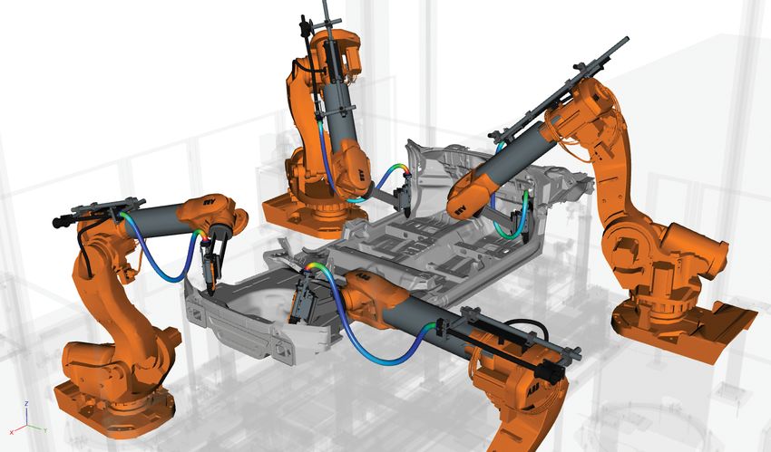
Path Optimization for Multi-Robot Station Minimizing Dresspack Wear
JONAS KRESSIN

c JONAS KRESSIN, 2013

Master’s Thesis EX013/2013
Department of Signals and Systems
Division of Automatic Control, Automation and Mechatronics
Chalmers University of Technology
SE-412 96 Göteborg
Sweden
Telephone +46 (0)31-772 1000

This Master’s Thesis was carried out at Fraunhofer Chalmers Research Centre for In-
dustrial Mathematics in Göteborg, Sweden.

Cover:
IPS simulation of stud welding station with dresspack bending moment analysis.
Abstract

When dealing with off-line programming of industrial robots there are sophisticated soft-
wares available for planning of the robot paths, one being Industrial Path Solutions (IPS)
developed by the Fraunhofer Chalmers Centre. One thing that is not taken into account
when finding the robot paths is potential wearing on the robots’ cable dresspacks. Since
dresspacks wearing out is very expensive both in material cost and cost from downtime,
there is a need for incorporating dresspack wear consideration when making the auto-
matic path planning.

This thesis addresses the problem of finding robot paths that are less damaging for the
dresspack, and the result consists of three different methods for dealing with this prob-
lem. The first method involves computationally efficient restrictions of the robot joint
values in order to avoid damage to the dresspack. The second method deals with the
issue of finding cable configurations that are robust to movements, since only robust
configurations should be used in the final sequences. Finally, the third method involves
a function that measures the cable wear as a cost, to then be minimized when doing the
automatic path planning.

The three methods are tested and evaluated individually on a test case in IPS. The tests
show that with the cable wear consideration, the robot takes different paths with lower
values of the wearing measures than the case without cables. It is concluded that with
some improvements of the methods, they can be combined into a fully implementable
solution.

Keywords: cable wear minimization, robot cable simulation, path planning, joint re-
strictions, robust cable configurations, cable wear cost function.

                            , Signals and Systems, Master’s Thesis EX013/2013            I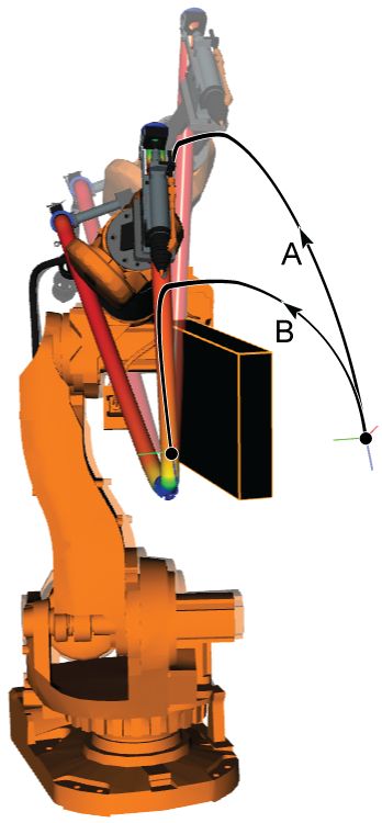
Acknowledgements
First of all I would like to thank my supervisors Daniel Segerdahl, MSc, and Tomas Her-
mansson, MSc, for their most valuable input and support throughout this thesis work. I
would also like to thank Robert Bohlin, Phd, for rewarding discussions on path planning
and optimization, and Johan Carlson, Phd and Director, for his guidance and support
throughout the work. I would also like to express my gratitude to my supervisor and
examiner from Chalmers, professor Bengt Lennartson, for his interest in this thesis.

Further on, I want to thank Mathias Sundbäck, Mikael Andersson and Johan Segeborn
at the Manufacturing Engineering department at Volvo Cars in Göteborg. Your welcom-
ing attitude helped me gain invaluable insight of the challenges with dresspack wear, as
well as rewarding on-site experience of the problems.

Last but not least I want to express my gratitude towards everyone else at FCC that
has helped me. The including atmosphere and willingness to help has really contributed
a lot to my work.

                                                                       Göteborg May 2013
                                                                             Jonas Kressin

II                         , Signals and Systems, Master’s Thesis EX013/2013
Contents
1 Introduction 1
1.1 Background . . . . . . . . . . . . . . . . . . . . . . . . . . . . . . . 1
1.2 Purpose and goal . . . . . . . . . . . . . . . . . . . . . . . . . . . . 2
1.3 Delimitations . . . . . . . . . . . . . . . . . . . . . . . . . . . . . . 2
1.4 Summary . . . . . . . . . . . . . . . . . . . . . . . . . . . . . . . . 3
2 Theory 4
2.1 Robot dresspacks . . . . . . . . . . . . . . . . . . . . . . . . . . . . 4
2.2 Cable modeling . . . . . . . . . . . . . . . . . . . . . . . . . . . . . 4
2.3 Robot kinematics . . . . . . . . . . . . . . . . . . . . . . . . . . . . 5
2.4 Path planning . . . . . . . . . . . . . . . . . . . . . . . . . . . . . . 7
2.5 Optimization . . . . . . . . . . . . . . . . . . . . . . . . . . . . . . 8
2.6 Summary . . . . . . . . . . . . . . . . . . . . . . . . . . . . . . . . 9
3 Methodology 10
3.1 Finding causes for cable wear . . . . . . . . . . . . . . . . . . . . . 10
3.2 Methods for implementing solutions . . . . . . . . . . . . . . . . . . 10
3.2.1 Joint restrictions . . . . . . . . . . . . . . . . . . . . . . . . 11
3.2.2 Robust cable configurations . . . . . . . . . . . . . . . . . . 11
3.2.3 Cable wear cost function . . . . . . . . . . . . . . . . . . . . 11
3.3 Test case evaluation . . . . . . . . . . . . . . . . . . . . . . . . . . . 12
3.4 Summary . . . . . . . . . . . . . . . . . . . . . . . . . . . . . . . . 13
4 Proposed Solution and Results 14
4.1 Joint restrictions . . . . . . . . . . . . . . . . . . . . . . . . . . . . 14
4.2 Robust cable configurations . . . . . . . . . . . . . . . . . . . . . . 17
4.3 Cable wear cost function . . . . . . . . . . . . . . . . . . . . . . . . 21
4.4 Test case evaluation . . . . . . . . . . . . . . . . . . . . . . . . . . . 24
4.5 Summary . . . . . . . . . . . . . . . . . . . . . . . . . . . . . . . . 26
, Signals and Systems, Master’s Thesis EX013/2013 III5 Discussion and Conclusion 27
5.1 Joint restrictions . . . . . . . . . . . . . . . . . . . . . . . . . . . . 27
5.2 Robust cable configurations . . . . . . . . . . . . . . . . . . . . . . 28
5.3 Cable wear cost function . . . . . . . . . . . . . . . . . . . . . . . . 29
5.4 Concluding remarks . . . . . . . . . . . . . . . . . . . . . . . . . . . 30
Bibliography 32
A Cable wear test case plots 33
IV , Signals and Systems, Master’s Thesis EX013/2013Chapter 1
Introduction
This chapter presents the background to this Master’s Thesis, including motivations
from industry. It also states the purpose and goal as well as delimitations.
1.1 Background
In time demanding robotic applications it is of great interest to find an optimized way
to perform a given task. One example is robot welding in car industry, where a given
set of welds are to be done and a set of stations and robots are given to do the welds.
The task is to find which robot should do which welds, and in what order, with a goal
to minimize the total time. Fraunhofer-Chalmers Research Centre for Industrial Math-
ematics (FCC) has developed a path planning software called Industrial Path Solutions
(IPS), which among many other features performs exactly this task. In excess of this,
IPS also supports simulation of flexible components (cables).
One thing that IPS has not been taking into account when doing the automatic path
planning is potential wearing of the robot’s cable dresspack. This wearing can be e.g.
that
• the cable hits some static geometry (e.g. sharp sheet metal on the car).
• the cable is bent in a bad way.
• the cable gets stuck somewhere and then tugged.
Damaged cable dresspacks are very expensive, both due to high costs for buying new
dresspacks and in particular stop in production. According to a study at Volvo Cars,
47% of the robot dresspacks wore out faster than the promised life length of one year
[1]. Out of all dresspack related breakdowns, 61% were considered to be major, i.e.
≥ 30 min [2]. The study also showed an existing potential to improve the situation,
with an estimation of 14% wear out instead of 47% if appropriate actions were to be
taken. Besides this, the robotic cable protection company REIKU claims that ”Almost
, Signals and Systems, Master’s Thesis EX013/2013 11.2. Purpose and goal
85% of Robotics and Automation ”downtime” can be directly attributed to cable or hose
failure” [3]. Also [4] and [5] report that failing cables is the foremost cause of downtime
for industrial robots.
The study at Volvo Cars showed that for some robots the dresspack never wore out
during the study period, whereas for others it wore out up to six times. Based on this
and insights from matter experts, it was established that the root cause likely was that
proper optimization of the robot path had never been performed [1]. Therefore, if the
dresspack wear would be considered at an early stage of planning, that could have a
significant effect on the robot breakdowns.
Modeling of robot dresspacks has been done in previous works, like e.g. in [6]. Here a
cable was modeled on a roller hemming robot and various simulations were performed.
The simulations included analyses of length, curvature, bending, tension and shearing.
Although the simulations did include analyses related to wearing, the focus was on
mounting and dresspack design rather than wearing minimization through path opti-
mization.
1.2 Purpose and goal
The purpose of this Master’s Thesis is to derive methods to minimize cable wear when
doing the automatic off-line programming in IPS. Questions to be answered are:
• Do the methods perform as intended?
• In excess of these methods, what more is needed for a commercially acceptable
solution?
The goal is to evaluate and verify functionality individually for each method, to then
conclude whether the methods can be combined to minimize dresspack wear on a multi-
robot station.
1.3 Delimitations
Since this Master’s Thesis is part of a collaboration between other projects, and since
some simulation features are currently not fully developed, the following is not included
in the goal and proceedings:
• The mathematical modeling of a cable (already implemented in IPS).
• Compilation of the path planning algorithm (already implemented in IPS).
• Simulation of dynamical behavior of a cable (effects due to acceleration, not fully
developed).
2 , Signals and Systems, Master’s Thesis EX013/20131.4. Summary
1.4 Summary
It has now been established that dresspack wear is a profound problem in industry, and
that dresspack wear consideration in the automatic off-line programming could have a
significant effect on robot breakdowns. To deal with the problem of cable wear, this
thesis aims at deriving methods for minimizing cable wear when doing the automatic
off-line programming, with the delimitations as stated in the previous section. Before the
derivation of these methods, Chapter 2, Theory will provide a brief theory foundation
with some general knowledge about robots, path planning and dresspacks.
, Signals and Systems, Master’s Thesis EX013/2013 3Chapter 2 Theory This chapter provides a brief theory foundation for this Master’s Thesis. The purpose is to provide general knowledge on the topics of robot dresspacks, cable modeling, robot kinematics, path planning and optimization. 2.1 Robot dresspacks For an industrial robot to be able to perform a task it needs some kind of tool. A tool can be e.g. a welding gun, a spray painting tool or a gripper. Each type of tool requires one or several types of resources, like e.g. electricity, pneumatics, material feeding or information exchange. To supply the tool with its resources there is a bundle of cables and hoses connecting to the tool, called a dresspack. The conventional way of routing a dresspack is externally along the upper arm, external dressing [7]. This routing is best suited for installations with low performance and low wrist movement complexity [8], but is still common among higher performance applica- tions. The problem with the external dressing is that it occupies space along the robot arm, which increases the possibility of collision with surrounding geometry. Another problem is the swinging motions of the dresspack, which causes wearing [7]. As a com- plement to the external dressing, internal dressing or integrated dresspack has emerged on the market. The internal dressing runs inside the robot upper arm and through the robot wrist, occupying much less space than the external. This makes the offline programming much easier, since the robot movements no longer need to be restricted because of the dresspack [8]. Also, since the swinging movements are avoided the wearing is significantly decreased [8]. 2.2 Cable modeling To simulate the dresspacks as slender, flexible objects, a mahematical model of a cable is needed. A cable or hose can be modeled as a slender one dimensional elastic object with 4 , Signals and Systems, Master’s Thesis EX013/2013
2.3. Robot kinematics

undeformed cross section, for both large and small deformations [9]. The characteristic
deformed shape of a cable is captured in a so called Cosserat rod, which can be seen as
a slender beam. The Cosserat rod is parameterized by arc length s (see Figure 2.1), and
is defined by the frames R(s) = (d1 ,d2 ,d3 ) defining the cross section orientations, and a
center curve ϕ(s) going through the center of the cross sections. The frame vectors d1 ,
d2 and d3 are orthonormal; d1 and d2 span the cross-section plane and d3 is the cross-
section normal. To acquire the deformed shape, each material point in the un-deformed
cable is mapped to the deformed via the deformation mapping

                                    χ : [0,L] × A 7→ R3                                     (2.1)

where

                        χ(s,ξ1 , ξ2 ) = ϕ(s) + ξ1 · d1 (s) + ξ2 · d2 (s)                    (2.2)

Here A is the cross-section and ξ1 ,ξ2 are planar coordinates in A.

                                                                  χ (s, ξ1 , ξ2 )

                                          d1
                                                     d3
                                φ

                                           d2
              Figure 2.1: A cable segment represented as a Cosserat rod [10].

2.3     Robot kinematics
Robot kinematics is about controlling the positions, velocities and accelerations of the
links of a manipulator, which in the case of an industrial robot is a robot arm [11]. The
links are the rigid bodies that the arm is built up by, and each link is manipulated by a
revolute joint. Link zero (the base) is static, link one is attached to joint one, link two
to joint two etc. Figure 2.2 shows a typical joint setup for a six axis industrial robot,
where link n connects joints n and n + 1 for n = 1...5. The last link connects joint six
to a tool attachment location called a tool plate.

To acquire the position and orientation of the tool plate relative to the robot base, a
method of multiplying transformation matrices is used [11]. The relation between link

                            , Signals and Systems, Master’s Thesis EX013/2013                  5
2.3. Robot kinematics
Axis 5 Axis 6
Axis 4
Axis 3
z
Axis 2 y
x
Axis 1
Figure 2.2: Typical joint setup for an industrial robot with six axes (joints).
n and n + 1 is described by the transformation matrix
xx yx zx px
n
xy yy zy py
Tn+1 =
(2.3)
xz yz zz pz
0 0 0 1
which consists of one rotation (x,y,z) and one translation (px ,py ,pz ) part. The transfor-
mation matrix of the tool plate, called the hand frame (H), relative to the base (R) is
then obtained as
R
T H = R T 1 1 T 2 . . . n−2 T n−1 n−1 T H (2.4)
As an example, consider again the robot in Figure 2.2. The transformation matrix for
link two is obtained as
R
T 2 = R T 1 1 T 2 = [T RAN S(x,l1 )ROT (z,j1 )][T RAN S(z,l2 )T RAN S(x,l3 )ROT (y,j2 )]
cos(j1 ) − sin(j1 ) 0 l1 cos(j2 ) 0 sin(j2 ) l3
sin(j1 ) cos(j1 ) 0 0 0 1 0 0
=
0 0 1 0 − sin(j2 ) 0 cos(j2 ) l2
0 0 0 1 0 0 0 1
cos(j1 ) cos(j2 ) − sin(j1 ) cos(j1 ) sin(j2 ) l3 cos(j1 ) + l1
sin(j1 ) cos(j2 ) cos(j1 ) sin(j1 ) sin(j2 ) l3 sin(j1 )
=
(2.5)
− sin(j2 ) 0 cos(j2 ) l2
0 0 0 1
6 , Signals and Systems, Master’s Thesis EX013/20132.4. Path planning
where l1 , l2 , l3 are lengths and j1 , j2 are joint angles. The method described above is
referred to as direct kinematics, i.e. finding the transformation matrix of the hand
frame given the robot joint values. To do the opposite, i.e. to find the joint values
given the hand frame transformation, is called solving the inverse kinematics and is
more complicated. There are several different algorithms available to solve the inverse
kinematics, one heuristic being to put the manipulator transformation matrix R T H equal
to the general transformation matrix in (2.5), and then solving for specific elements.
However there might not be one single solution for a specific transformation, but rather
several solutions. This is called redundancy, and is a common occurrence when solving
the inverse kinematics. There can also be infinitely many solutions; this is referred to as
degeneracy.
2.4 Path planning
With a description of how the kinematics affect the robot position, a framework for plan-
ning of the robot paths can now be derived. To understand what path planning is one
can consider the Piano Mover’s Problem [12]. Consider a 2-or 3-dimensional drawing
or model of a house and a piano. The problem is to move the piano from one room to
another in an efficient way, without colliding with anything. In robotics this problem
translates to moving the robot from one configuration to another without colliding with
any static geometry or with the robot itself.
To reduce complexity and pave the way for further planning theory, the robot configura-
tions are represented in a configuration space (C-space) [12]. A configuration expresses
the position of the robot in terms of its joint angles, and given a sample point in C-space
it is possible to check whether the robot is in collision or not. With the C-space rep-
resentation in order, the problem is now reduced to finding a collision free path from a
start configuration, qinit , to a goal configuration, qgoal , or determine that no such path
exists.
One method for finding a collision free path between qinit and qgoal , is the Probabilistic
Roadmap Method (PRM) [13]. The main idea is to first do a preprocessing step to acquire
a network (roadmap) of randomly distributed collision free configurations, and then to
connect qinit and qgoal via the network nodes (see Figure 2.3). If there is no possible
way of connecting the configurations without colliding with any obstacles, the method
has failed to find a feasible path and a denser sampling is needed. It is shown in [13]
that as time tends to infinity and the number of sample points increases, the probability
of classifying a feasible problem as infeasible tends to zero. This is called probabilistic
completeness and is a key feature for a planning algorithm.
, Signals and Systems, Master’s Thesis EX013/2013 72.5. Optimization
Figure 2.3: Example of a probabilistic roadmap from qinit to qgoal [13].
2.5 Optimization
As described in Section 2.4, the path planning procedure involves random distribution of
points in the configuration space. Since this randomness might lead to strange, ”jerky”
paths for the robot, there is a need for some kind of smoothing of the paths. In [13]
a smoothing procedure is suggested, where new points are added around the acquired
path, upon which a shorter feasible path is searched for locally around the old one. When
also considering e.g. time, and eventually cable wear, this smoothing procedure can be
seen as a multi-objective optimization problem.
The term ”to optimize” is explained in [14] as ”to do something as well as is possible”. In
mathematical terms this translates into altering a set of variables, in order to minimize
or maximize an objective function, without violating certain constraints. When dealing
with minimization, the objective function is often referred to as a cost function. With
this terminology the problem can intuitively be translated into to do something with as
low cost as possible or to do something as cheap as possible. For the smoothing problem,
the cost consists of several sub-costs, like e.g. traveling distance cost and time cost. The
objective is then to minimize the total cost by selecting sample points in the configura-
tion space.
When selecting the sample points, it makes sense to select points that result in a lower
value for the cost function. The direction in the configuration space that gives a lower
cost is called a direction of descent. A sufficient condition for descent, given in [14],
is that for a cost function f : Rn → R ∪ {+∞} in C 1 around a point x, for which
f (x) < +∞, there exists a vector p ∈ Rn such that
∇f (x)T p < 0 (2.6)
holds. p is then a descent direction with respect to f at x. An intuitive and graphical
interpretation of this is to move in the opposite direction of the gradient of the cost
function, or rather in a direction > 90◦ away from the gradient.
8 , Signals and Systems, Master’s Thesis EX013/20132.6. Summary
2.6 Summary
The topic of path optimization for robots considering dresspack wear covers several areas
of expertise, of which a significant part has been briefly presented in this chapter. The
most important parts for further understanding of this thesis are the robot kinematics
and path planning and optimization; in particular the robot joint setup and the un-
derstanding of having C-space configurations as variables for the optimization. With a
theory foundation in order, the problem of finding robot paths with minimized dresspack
wear can now be approached in Chapter 3, Methodology.
, Signals and Systems, Master’s Thesis EX013/2013 9Chapter 3 Methodology This chapter presents the methods and procedures used in this Master’s Thesis. The structure follows a chronological order, starting with finding causes for cable wear, then finding methods for implementing solutions and finally formulating a method- ology for a test case evaluation. 3.1 Finding causes for cable wear In order to detect and avoid cable wear, it was essential to acquire knowledge about the cause of the wearing. To get a broad picture, interviews and discussions were held with simulation experts and robot programmers with hands-on experience from cable wear. Since the framework for this Master’s Thesis was to perform path optimization, the causes needed to be filtered out to only include the ones that could be affected by the robot path. This excluded wearing causes like e.g. poor rigging of the dresspacks and badly chosen dresspack types for a given robot application. These kinds of wearing causes cannot be dealt with through path optimization, but need to be addressed by the dresspack designers. Further on, the studies in [1] and [2] pointed out and confirmed the causes acquired from the interviews. In connection with the interviews, company visits to Volvo Cars were made, at which a deeper knowledge and understanding of the problems was acquired. 3.2 Methods for implementing solutions To achieve the main goal of finding paths with reduced cable wear, the work was divided into different subtasks. The interviews revealed that some problems were best solved with path optimization considering cable wear, but also that some wearing could be avoided with computationally efficient restrictions on the robot joint values. It was also established that some method for determining robustness of configurations was needed. 10 , Signals and Systems, Master’s Thesis EX013/2013
3.2. Methods for implementing solutions

3.2.1   Joint restrictions
From the interviews it was found that some hands-on solutions, or ”rules of thumb”,
that the robot simulators at Volvo were using could be translated into computationally
efficient rules for joint restrictions. This meant that some wearing could be avoided by
restricting the values of the robot joint angles. To translate the ”rules of thumb” into
computer implementable rules, an understanding of how the joint values affect the cable
needed to be found. This understanding lead to geometrical relationships between the
joint values and the cable shape, which in turn could be modeled using mathematical
geometry.

3.2.2   Robust cable configurations
When performing automatic path planning without any cables, the location of the robot
is deterministic, given a certain robot configuration. This is because the robot consists
of rigid bodies and the surrounding geometry is static. However when attaching a cable
to a robot, the shape of the cable is not deterministic, given a robot configuration. The
shape might depend on the previous traveling path of the cable.

In the first step of the automatic path planning, IPS finds the set of all possible robot
configurations for reaching a weld point. Since the path to reaching such a point at this
stage has not been decided yet, it was necessary to only include points where the cable
shape could be determined regardless of previous traveling path. A cable configuration
is specified by the rotation and translation of the cable’s nodes (attachment points), and
it is considered to be robust if the cable shape is roughly the same regardless of previ-
ous traveling path, or approach direction. To be roughly the same means in practice to
achieve cable shapes that may differ up to a certain maximum distance from each other,
regardless of approach direction.

To find a method for determining robustness of cable configurations, the relationship
between the physical design of the robot and the cable configurations was examined. By
knowing how the robot joints affect the cable configurations, an algorithm for mapping
robustness could be developed. To verify the algorithm, a script was written in the
programming language Lua. In IPS, Lua-scripts can be used for importing pre-defined
cables, changing transformations of the cable’s nodes and saving information about the
cable shape. To manipulate the node positions and orientations, the method of multi-
plying transformation matrices from Section 2.3 was used.

3.2.3   Cable wear cost function
The cable wearing that could not be avoided with the computationally efficient joint
restrictions needed to be included and considered in the path planning algorithm. Since
the already existing path optimization in IPS was subject to several objectives, like e.g.
time minimization, smoothness and energy consumption, the introduction of the cable

                            , Signals and Systems, Master’s Thesis EX013/2013          11
3.3. Test case evaluation wear minimization needed to be done without removing these other objectives. There- fore the most suitable implementation was to construct a cost function, giving increasing cost with increasing cable wear. For this implementation the wearing causes needed to be translated to and expressed in measurable quantities. Because of the high complexity of the optimization problem, being both highly non- linear and non-convex, the existing algorithm does not search for a globally optimal solution [12]. Instead the algorithm starts by finding a nominal path, to then be locally optimized. It is in this local optimization that the cable wear was to be considered, together with the other criteria (time, smoothness etc). Since there are typically many different solutions to the path planning problem, of which many have similar cycle time, the algorithm might find a path with less cable wear but without a radical increase in cycle time. 3.3 Test case evaluation In order to evaluate the derived methods, a stud welding robot was chosen as a test case. The chosen robot was from the station that can be seen in the front page picture of this thesis. The stud welding robot is problematic when it comes to cable wear, since the dresspack has no retracting/feeding unit to pull back or feed out the cable when the robot moves. Instead the cable hangs down from the robot, increasing possibility of collision and twisting around the robot arm. To verify the functionality of the derived methods they were evaluated individually. To get the cable to resemble the reality as much as possible, the cable material parameters were acquired through data acquisition from a similar real robot and cable setup at a stud welding station at Volvo Cars. By measuring mass and length of the cable, the length density could be calculated as ρl = m/l. By then moving the robot to four different poses and taking pictures, the pictures could be compared to the simulation and the remaining parameters tuned to get the model to resemble the reality as good as possible. The dimensions and material parameters that were chosen are presented in Table 3.1. 12 , Signals and Systems, Master’s Thesis EX013/2013
3.4. Summary

                            Parameter             Value

                            Length                1740 mm
                            Radius                30 mm
                            Length density        1.25 kg/m
                            Bending stiffness     0.1 N m2
                            Tensile stiffness     1400 N
                            Torsional stiffness   0.1 N m2
                  Table 3.1: Cable dimensions and material parameters.

3.4    Summary
The methodology of this thesis consists of three major parts: finding causes for cable
wear, methods for implementing solutions and finally a test case evaluation. With these
three steps the cable wear will both be identified and dealt with through three different
methods. These methods handle the topics of: joint restrictions, robust cable configu-
rations and cable wear cost function, where the first and the last method handles the
actual cable wear reduction, and the second deals with the issue of finding non-robust
configurations. The three methods together with the test case evaluation represent the
outcome of this thesis, and they are all derived, evaluated and presented in Chapter 4,
Proposed Solution and Results.

                           , Signals and Systems, Master’s Thesis EX013/2013          13
Chapter 4
Proposed Solution and Results
This chapter presents a proposed solution as well as acquired test results of this Master’s
Thesis. First, a presentation of the three sub-results is given. The sub-results include
the topics of joint restrictions, robust cable configurations and cable wear cost
function. After this the three sub-results are tested on a selected test case, upon which
results are presented in test case evaluation.
4.1 Joint restrictions
A computationally efficient way to avoid bad cable behavior is to use joint restrictions.
By restricting the values of the robot joints in a clever way, some bad movements and
poses for the cable can be completely accounted for. The reason why this method is
computationally efficient, in relation to path planning robot and cable, is that a simple
condition check is done, upon which a joint value is allowed if the condition is true and
prohibited if it is false.
One example of bad behavior is if the cable twists too much around the robot arm,
which leads to high stress and possible snapping of the cable. To prevent this the robot
simulators at Volvo Cars use a ”rule of thumb” suggesting that the absolute value of the
angle sum of joints four and six must not exceed 270◦ , i.e.
| j4 + j6 |≤ 270◦ (4.1)
Inequality (4.1) is a simple condition check, where a given pair (j4 , j6 ) is allowed if and
only if (4.1) evaluates to boolean true.
Another bad behavior is when joints five and six are arranged in such a combination,
that the joint six cable support comes too close to the robot arm (see Figure 4.1(a)).
This results in the cable being crushed against the arm. To avoid this it is meaningful
to have a certain clearance from the tip of the cable support down to the robot arm.
This can be done by restricting the allowed space for joint five.
14 , Signals and Systems, Master’s Thesis EX013/20134.1. Joint restrictions
l β γ
α
h
a
m
α
(a) (b)
Figure 4.1: (a) j5 at critical angle, crushing the cable against the arm. (b) Corresponding
geometric figure.
The restriction on joint five is dependent on the angular value of joint six. For some
angles of joint six, joint five can be changed arbitrarily without endangering any crushing
of the cable, whereas for others a restriction is needed. One way to think of it is that it
is only at certain zones of joint six that joint five must be restricted. Assuming joint six
is in one of these zones, the restriction on joint five will depend on a function of joint
six. This is due to the geometry of the robot arm (approximated as a cylinder). Also,
since the cable support can be physically mounted in different initial angles relative to
joint six, the zones will depend on this mounting angle. Figure 4.2 gives an example of
the forbidden zones for joint five, as a function of joint six.
Forbidden zones for j5
150
Zone B
100
50
j5 [deg]
0
−50
−100
Zone A
−150
−300 −200 −100 0 100 200 300
j6 [deg]
Figure 4.2: Forbidden zones for joint five, with the cable support mounted in a −45◦ angle
(measured CW from joint six zero angle).
, Signals and Systems, Master’s Thesis EX013/2013 154.1. Joint restrictions
To determine the restriction function for joint five, the physical design of the robot is
examined. Figure 4.1(b) shows a geometrical sketch of the robot arm in Figure 4.1(a),
with m being the length of link five, l the length of the cable support and a the distance
from the tip of the support down to the centerline of link four. The angle α is directly
related to the value of joint five; α = −j5 when j6 is in zone A and α = j5 when j6 in
zone B. The distance a can be approximated as
a ≈ r cos(j6 + p) + c if j6 in zone A
a ≈ r cos(j6 + p + π) + c if j6 in zone B
where the parameters are described in Table 4.1. With explicit expressions for l, m and
a, α can now be written as
α=β+γ
−1 l a
= cos + cos−1
h h
−1 l −1 a
= cos √ + cos √ (4.2)
m2 + l 2 m2 + l 2
With a in (4.2) being a function of j6 , and with the relation j5 = −α (zone A) and
j5 = α (zone B), joint five can now be restricted with a function of joint six. Zone A
will yield a lower bound on j5 and zone B an upper bound, due to the physical design of
the robot. The restriction on joint five becomes
l r cos(j6 − p) + c
j5 ≥ fA (j6 ) = − cos−1 √ − cos−1 √ if j6 in zone A
m2 + l2 m2 + l2
(4.3)
l r cos(j6 − p + π) + c
j5 ≤ fB (j6 ) = cos−1 √ + cos−1 √ if j6 in zone B
2
m +l 2 m2 + l 2
(4.4)
where the parameters are summarized in Table 4.1.
Parameter Description
r Radius of link four (approximated as a cylinder).
m Length of link five.
l Length of cable support.
c Required clearance to link four.
p Angle for cable support. Measured CW from j6 zero angle [−180◦ , 180◦ ].
Table 4.1: Parameters for joint restriction function.
16 , Signals and Systems, Master’s Thesis EX013/20134.2. Robust cable configurations
Since the robot arm is approximated as a cylinder, the restriction functions in (4.3) and
(4.4) work best for (roughly) cylindrical robot arms. Although the upper arm of the
robot in Figure 4.1(a) is roughly cylindrical, the wrist close to link five is not. This is
why the cylindrical approximation can be replaced by a cuboid approximation. With
the cuboid approximation, the restrictions on joint five become
−1 l −1 r+c
j5 ≥ − cos √ − cos √ = −K if j6 in zone A (4.5)
m2 + l 2 m2 + l2
−1 l −1 r+c
j5 ≤ cos √ + cos √ = K if j6 in zone B (4.6)
m2 + l2 m2 + l2
where K is a (pre-calculated) constant for a given clearance c and r is now half the
height of the cuboid. The cuboid approximation is more accurate than the cylindrical
for shorter cable supports and/or large clearance, and also requires even less calculation
processing. To know which approximation to use, one can examine the tip of the cable
support when j5 is at its critical angle. If the tip is above the cylindrical part of the
robot arm, the cylindrical approximation is to be used, and if above the wrist the cuboid
approximation is chosen.
An easily implemented method for including all the joint restrictions is to combine them
into a single logical expression. In this section only two different types of restrictions have
been dealt with, but the implementation also works for a larger number of restrictions.
Using the cylindrical approximation for the restriction on joint five, the joint restrictions
from (4.1), (4.3) and (4.4) can be combined into the logical expression
[| j4 + j6 |≤ 270◦ ] ∧ [[j6 in zone A] ∧ [j5 ≥ fA (j6 )] ∨ [j6 in zone B] ∧ [j5 ≤ fB (j6 )]]
(4.7)
which can easily be implemented in computer code. The expression must evaluate to
boolean true for any given set of joint angles (j4 , j5 , j6 ), i.e. a given joint configuration
is allowed if and only if (4.7) is true.
4.2 Robust cable configurations
When determining robustness of cable configurations, the most straightforward way
might be to attach a dresspack to a robot and then test robustness for all possible com-
binations of the joint angles (j1 , j2 , j3 , j4 , j5 , j6 ). However this would result in too many
configurations to test (about 1.13 × 10¹⁵ for an angular resolution of 1◦ ). In this section
it is shown that only a subset of these configurations need to be tested, and an algorithm
for testing the configurations is derived. The developed method is also verified by finding
non-robust configurations for two different test cables.
To find out which of the configurations that can be excluded from the testing, one must
first examine how the physical design of the robot affects the movement of the cable.
, Signals and Systems, Master’s Thesis EX013/2013 174.2. Robust cable configurations
An industrial robot is limited to movement in six degrees of freedom. Considering only
the end part of a cable, that goes from link three to link six, the movements of joints
one, two and three will transform all cable nodes in a uniform fashion, i.e. as one rigid
unit. As an example, consider the robot and cable in Figure 4.3. Here the two rightmost
nodes are rigidly connected to link three, and the leftmost node to link six. In this case
joints one, two and three will move all cable nodes as one unit, whereas joints four, five
and six will only affect the leftmost node.
Figure 4.3: Robot with cable attached to links three and six.
Intuitively, a pure translation of the cable in Cartesian (x,y,z) will not affect the cable
shape. Similarly, rotating about the z-axis in Figure 4.3 will also not affect the cable
shape. Assuming the rotation in z is locked to the position in Figure 4.3, the cable will
only be able to rotate about the y-axis (since the robot cannot tilt sideways about the
x-axis). With these limitations, it is only of interest to study configurations as a result
from
• rotation of the entire cable about the y-axis (Ry ).
• movement of leftmost node by manipulating joints four, five and six (j4 ,j5 ,j6 ).
Since the only parameters determining the positions of the cable nodes are the ones just
described, a cable configuration can be defined by the configuration vector
v = (Ry ,j4 ,j5 ,j6 ) (4.8)
The condition is that the cable and robot setup is as above, i.e. that joints one, two
and three move all cable nodes as one unit, and that the robot is either floor- or ceiling
mounted.
With the desired configurations identified, an algorithm for measuring robustness for a
configuration can now be developed. As described in Section 3.2.2, a robust configuration
has roughly the same cable shape regardless of previous traveling path. Therefore, to
determine robustness the cable needs to be moved to a configuration along different
18 , Signals and Systems, Master’s Thesis EX013/20134.2. Robust cable configurations
paths. To keep down computational effort, a total of two paths are selected for the
robustness testing. This resulted in Algorithm 1. The idea is to first move the cable nodes
to the configuration to be tested, and then save the cable shape by saving Ns (x,y,z)-
sample points along the cable segment. By then decreasing the values of the configuration
vector v, followed by increasing back to the current configuration, a negative movement
has been made. Ideally the cable shape should now be exactly the same as before the
movement, and any too large deviations implies non-robustness. By then doing a positive
movement in a similar manner, two cable shapes have been acquired to be compared to
the initial shape. If, for any sample point, the distance to corresponding sample point
in the initial shape is greater than distance threshold dthresh , the configuration is non-
robust.
Algorithm 1 Configuration robustness mapping
1: V←∅ . Init non-robust configurations
2: for i ← 1, N do . For all N configurations
3: moveN odes(v(i)) . Move all nodes to config i
4: S0 = getShapeData() . Store initial shape
5: ◦ ◦ ◦
moveN odes(v(i) − (20 ,100 ,100 ,100 )) ◦ . Do negative movement
6: moveN odes(v(i)) . Move back to config i
7: S1 = getShapeData() . Store shape
8: ◦ ◦ ◦
moveN odes(v(i) + (20 ,100 ,100 ,100 )) ◦ . Do positive movement
9: moveN odes(v(i)) . Move back to config i
10: S2 = getShapeData() . Store shape
11: for j ← 1, Ns do . For all cable segment sample points
12: if d(S0 (j), S1 (j)) ≥ dthresh or d(S0 (j), S2 (j)) ≥ dthresh then
13: V ← V ∪ v(i) . Save non-robust config
14: end if
15: end for
16: end for
To verify that the algorithm produced a reasonable mapping of non-robust configura-
tions, it was tested with two different cables. To resemble a real case scenario, one spot
welding cable and one stud welding cable were used (cable A and B, respectively). Figure
4.4 shows how the two cables were attached to the robot links. The configurations were
achieved by taking all possible permutations of
• Ry from −225◦ to 115◦ increment 20◦
• j4 from −180◦ to 180◦ increment 30◦
• j5 from −110◦ to 110◦ increment 30◦
• j6 from −180◦ to 180◦ increment 30◦
, Signals and Systems, Master’s Thesis EX013/2013 194.2. Robust cable configurations
This yielded 24,336 unique configurations. For each configuration the maximum devia-
tion from the initial shape was calculated using Algorithm 1 and then plotted (see Figure
4.5). With the deviation threshold dthresh = 100 mm, a total of 6% (A) and 5% (B) of all
configurations were found to be non-robust. For cable A some patterns for non-robust
configurations could be seen, e.g. the combination (j4 , j5 , j6 ) = (−150◦ , −110◦ , 0◦ ), which
always yielded non-robust configurations (except for Ry = 55◦ ). Also, Ry = 75◦ yielded
non-robust configurations, regardless of the other joint values. However for cable B no
definite pattern could be established, since the occurrence of non-robust configurations
was more random than for cable A. Although no definite pattern was found, an increase
in the amount of non-robust configurations for Ry close to ±90◦ could be seen. For these
configurations 17% could be considered to be non-robust.
(a) (b)
Figure 4.4: (a) Cable A and (b) cable B, with marked link attachments.
Deviation from init shape per configuration Deviation from init shape per configuration
1600 1000
Ry = 75° 900
1400
800
Maximum deviation [mm]
Maximum deviation [mm]
1200
700
1000
600
800 (-150°,-110°,0°) 500
400
600
300
400
200
200
100
0 0
0 0.5 1 1.5 2 2.5 0 0.5 1 1.5 2 2.5
Config number 4 Config number 4
x 10
x 10
(a) (b)
Figure 4.5: Simulation results for (a) cable A and (b) cable B. The red dashed line indicates
the threshold between robust and non-robust configurations. The green point clusters in (b)
indicate Ry = ±90◦ .
20 , Signals and Systems, Master’s Thesis EX013/20134.3. Cable wear cost function
4.3 Cable wear cost function
Cables wearing out involves several different types of wearing factors, and as described
in Section 3.1 this thesis focuses on the ones that are affectable by the robot path. In-
terviews with simulation experts and on-line robot programmers revealed that the main
factor is contact with static geometry (e.g. the car body). When hitting a sharp metal
edge at high speed this type of damage is amplified, but since this thesis is delimited to
only include static cable simulations, this phenomenon will not be accounted for. How-
ever, this effect can be reduced by increasing the clearance threshold when doing the
automatic path planning.
Another type of wearing that was shown from the interviews and from [1] is bending of
the cable. Excessive bending can lead to insulation cracking and damage to the cable
[15], and one major cause for this is bad robot paths. By avoiding robot paths with
excessive bending this kind of damage can be reduced. A special siuation identified in
[1] is improper mounting of the cable that may be damaging independent of the path.
This could easily be detected by static analysis, and does not require path optimization.
A third problem that was found during one of the study visits at Volvo Cars is when the
cable gets stuck somewhere on the robot arm, and then gets tugged by the robot. This
introduces high stress on the cable and could lead to severe damage at the attachment
points or on the cable itself. This kind of problem might arise when the cable hangs loose,
without any retracting/feeding unit to pull back or feed out cable when the robot moves.
For the three major wearing causes; contact, bending and tugging, to be minimized, they
need to be detectable and measurable in IPS. As for the contact, the shortest distance
to any static geometry can be used as a measure. This being zero is equivalent to being
in contact, and anything else can be directly related to a desired clearance. Since there
will always be some amount of uncertainty in the simulation compared to the reality,
it is desirable to have a certain clearance between the cable and surrounding geometry.
Also, as previously mentioned, clearance is a way to take uncertainties due to dynamical
effects into account.
The deformed shape from bending a cable can be determined completely by the bending
radius R [16]. A very tight bend is undesirable and can be detected by a very small
bending radius. To avoid tight bending but allow smoother bending, the curvature is
a natural bending measure, being the inverse of the radius (κ = 1/R). For a bending
radius going to zero the curvature will go to infinity, which used as a cost will prevent
very tight bends.
To measure or detect tugging, the tension force of the cable can be used. The tension
force is the longitudinal force in the cable and in normal cases, i.e. when the cable suffers
no drastical pulling, it is rather small. However, when the cable gets stuck and tugged
, Signals and Systems, Master’s Thesis EX013/2013 214.3. Cable wear cost function
the tension force grows fast with increased tugging.
With acquired measures of cable wear, it is possible to construct a cost function giving
increasing cost with increased wearing. Since the already existing path optimization in
IPS utilizes minimization of other objectives like e.g. time, it is suitable to include the
cable wear cost function as a term among these other costs. The overall goal of the
optimization is to optimize the path by tuning a set of N abstract configuration vectors
defining the path. These configuration vectors are considered to be the variables of the
optimization, and together they form the path
γ
1
γ
2
Γ= . (4.9)
..
γN
where γi is configuration vector i. Note that γi is not the same configuration vector as
v in Section 4.2, but rather a more general vector with all joint values included.
When constructing the cost function it is not suitable to use the acquired measures
directly, because of reasons as follows. Since the cable is typically not straight under
normal bending circumstances, the curvature must have a lower threshold for the bend-
ing penalty to take effect. Similarly for the shortest distance measure, being further
away than a specified clearance must not result in any penalty. This is why the shortest
distance measure needs an upper threshold, which is equal to the desired clearance.
To ensure that large violations of the cable wear factors result in extra penalization, all
factors are squared. By then multiplying each factor with a cost weight, the optimization
can be tuned to take each factor into more or less consideration. Summing the three
weighted terms together, the cable wear cost function for configuration γi becomes
C(γi ) = wκ · max(0,κ(γi ) − κ0 )2 + wF · F (γi )2 + wd · min(0,d(γi ) − c)2 (4.10)
| {z } | {z } | {z }
Cκ (γi ) CF (γi ) Cd (γi )
where the parameters are presented in Table 4.2 and
• κ(γi ) is the largest curvature of the cable,
• F (γi ) is the largest tension force,
• d(γi ) is the shortest distance to any static geometry.
22 , Signals and Systems, Master’s Thesis EX013/20134.3. Cable wear cost function
Parameter Description
κ0 Smallest curvature for the curvature penalty to take effect.
wκ Cost weight, curvature.
wF Cost weight, tension force.
wd Cost weight, shortest distance.
c Desired clearance to surrounding geometries.
Table 4.2: Parameters for cable wear cost function.
For better understanding of how the three terms Cκ (γi ), CF (γi ) and Cd (γi ) contribute
to the overall cost, they have been plotted individually as functions of their respective
wearing factors (see Figure 4.6). Curvatures that are ≤ κ0 are neglected, and curvatures
going to infinity result in the cost going rapidly to infinity. Tension forces going to
infinity gives cost going rapidly to infinity, and the distance cost is always in the interval
[0, wd · c2 ]. By not having a distance cost going to infinity for distance going to zero,
contact with surrounding geometry is allowed, however still penalized.
2
wd • c
CF(γi)
Cd (γi)
Cκ(γi)
0 0 0
0 κ0 0 0 c
κ(γ ) F(γ ) d(γ )
i i i
(a) (b) (c)
Figure 4.6: The three cost terms in the cable wear cost function (a) Cκ (γi ), (b) CF (γi )
and (c) Cd (γi ).
, Signals and Systems, Master’s Thesis EX013/2013 234.4. Test case evaluation
4.4 Test case evaluation
To verify the functionality of the methods, each method was evaluated individually on a
test case. As described in Section 3.3, the chosen test case is a stud welding robot from
the station on the thesis front picture.
To acquire joint restrictions, the physical design of the robot was examined. In this case
the joint restriction for the cable support is not necessary, since j5 and j6 can be changed
arbitrarily without endangering any crushing of the cable. However the restriction from
Inequality (4.1) can be used with some modification to account for a different initial
mounting position of the dresspack. Since joints four and six are both turned 180◦ for
the home configuration, the joint restriction becomes
j4 + j6 ≥ 90◦ (4.11)
Moving on to the cable configurations, a mapping was done using Algorithm 1 to acquire
the non-robust configurations. The joint angles were achieved by taking all possible
permutations of
• Ry in 20 steps evenly distributed around 0◦ from −180◦ to 180◦
• j4 in 15 steps evenly distributed around 0◦ from −180◦ to 180◦
• j5 in 15 steps evenly distributed around 0◦ from −110◦ to 110◦
• j6 in 15 steps evenly distributed around 0◦ from −180◦ to 180◦
This resulted in 67,500 different configurations. With a non-robustness threshold dthresh =
100 mm, a total of 5,743, or 9%, can be considered as non-robust. Figure 4.7 shows how
the amount of non-robust configurations varies with Ry . As in the case with cable B in
Section 4.2, the amount increases for Ry close to ±90◦ .
Amount of non−robust configurations
18
16
Non-robust configurations [%]
14
12
10
8
6
4
2
−180 −90 0 90 180
Ry [deg]
Figure 4.7: Amount of non-robust configurations for Ry .
24 , Signals and Systems, Master’s Thesis EX013/20134.4. Test case evaluation
To evaluate the cable wear cost function, three different scenarios were constructed for
curvature, tension force and distance costs. For each cost term evaluation, the cost
weights for the two remaining terms were put to zero. Each scenario resulted in a plot,
comparing performance between the two cases; with and without cable wear costs. These
plots are presented in Appendix A.
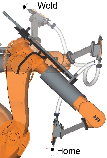
For the curvature evaluation, a scenario where one end of the cable was attached to the
robot tool and the other statically fixed in mid-air, was constructed (see Figure 4.8).
The robot was to move between the two configurations Home and Weld, at which both
yielded rather small curvature for the cable. However in the case without curvature cost,
the cable underwent sharp bending in the middle of the path when the tool passed close
to the static cable node. By introducing the curvature cost from Equation (4.10), with
wκ = 1 and κ0 = 8 [1/m], the path was altered to allow smooth bending but try to avoid
bending where κ ≥ 8 [1/m]. This resulted in a 62% decrease in maximum curvature
during the path.
Figure 4.8: Curvature test case. The robot moves from Home, via Weld and then back to
Home.
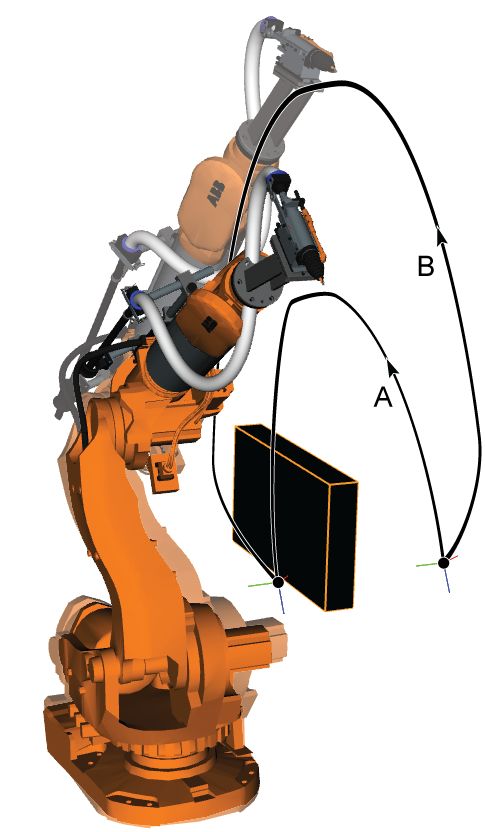
In the second scenario the tension force is evaluated. In this scenario the robot was to
move between two points without colliding with a cuboid obstacle (see Figure 4.9(a)).
By having a cable node firmly attached underneath the cuboid, movement of the robot
above the cuboid introduces high tension force. With a desired robot clearance of 500
mm the path planning algorithm finds a path high above the cuboid, when no force cost
is considered (path (A) in Figure 4.9(a)). However when the force cost is introduced
with wf = 1 × 10⁻⁵ , the path gets closer to the cuboid ((B) in Figure 4.9(a)). This is
because it is less costly to violate the clearance than to have a high tension force. With
the force cost the maximum tension force decreased by 61%.
, Signals and Systems, Master’s Thesis EX013/2013 254.5. Summary
The third scenario is for the distance cost evaluation. Again the robot was to move be-
tween two points, both with and without the distance cost (see Figure 4.9(b)). Without
the cost, the robot moves closer to the obstacle (path (A)) and with the cost, the robot
moves both higher above and further away from the sides of the obstacle (path (B)).
The cost parameters for path (B) were wd = 100 and c = 1 [m].
(a) (b)
Figure 4.9: (a) Tension force test case. Path (A) is without cost and path (B) is with
cost. The cable is subject to a tension force analysis with hot and cold colors for higher and
lower tension force, respectively. (b) Shortest distance test case. Path (A) is without cost
and path (B) is with cost.
4.5 Summary
This chapter has presented the results and outcome of this thesis, consisting of two
methods for cable wear reduction, one method for dealing with non-robust configura-
tions and finally a test case evaluation. The two methods for reducing cable wear involves
one computationally efficient method, joint restrictions, and one computationally more
cumbersome method, cable wear cost function. The mapping of non-robust configura-
tions is a difficult but essential part of the overall solution, and the test case evaluation
shows how the methods perform individually. Now a discussion about the results as well
as conclusions and suggestions for future work will be given in Chapter 5, Discussion
and Conclusion.
26 , Signals and Systems, Master’s Thesis EX013/2013Chapter 5
Discussion and Conclusion
In this chapter a discussion about the result is given. Also, conclusions and suggestions
for future work are presented. The structure is built on the three sub-results from the
result chapter; joint restrictions, robust cable configurations and cable wear cost
function, and then ended with some summarizing concluding remarks.
5.1 Joint restrictions
The main reason for restricting the joint values to avoid cable wear is the computa-
tional efficiency. By avoiding any collision checking and cable simulation, and simply
just checking the joint values, this is a highly efficient method. It is also beneficial con-
sidering implementation, since it is easy to check whether a certain joint value fulfills a
criterion, and to restrict it if it doesn’t. There is however a (small) drawback with this
method, and that is that it is not very general, but valid only for specific robot appli-
cations. For example, the restriction functions for joint five (4.3), (4.4), (4.5) and (4.6)
only work for robots with the specified cable support mounted on the tool plate. For a
robot application with different dresspack mounting, new options for joint restrictions
need to be examined.
Since the computational gains are so great for this method, it is worth spending some
extra time trying to find joint restrictions. When assessing a new dresspack and robot
setup, the first thing to check should be if there are any joint restrictions that can be
implemented to minimize wearing. With restrictions dependent on mounting parameters,
like e.g. the cable support angle, cable wear can be minimized with high computational
efficiency and with some generality and flexibility.
, Signals and Systems, Master’s Thesis EX013/2013 275.2. Robust cable configurations
5.2 Robust cable configurations
The justification for developing the robustness mapping algorithm was the fact that
non-robust cable configurations is a big problem. If one of the tasks, i.e. one of the
robot configurations for a certain weld point, results in a non-robust cable configuration,
the sequencing step in the working procedure will not be feasible. This means that it
will not be possible to change the order of the tasks or to alter the paths leading to
the non-robust configuration. Ignoring the non-robust configuration will make any cable
wear consideration in the path optimization inapplicable. If a non-robust configuration
is found among the robot tasks, one easy fix to this problem is to determine the task
order and perform the path planning for all tasks prior to the configuration, without
cable wear consideration. This will give usable but somewhat inferior results.
Since no previous research was found on cable robustness mapping, the procedure for
developing the algorithm was based on knowledge of the problem alone. Although veri-
fied with two different test cases, the algorithm can not be considered to be completely
validated. This is because some issues still need to be dealt with, like e.g.
• the definition for a non-robust configuration might be too vague.
• the choice of distance threshold dthresh is not trivial.
• it has not been shown that the two paths in the algorithm are enough for deter-
mining non-robustness.
This is why one suggestion for future work is to deal with these issues and refine the algo-
rithm. Since the definition for non-robustness implies having to test all possible traveling
paths to a configuration, a better definition is probably the first thing to investigate. By
proving some kind of completeness of the definition, e.g. having a high probability of
rightly classifying robustness by moving along a small number of ”bad enough” paths,
the robustness mapping should be implementable in a commercial context.
Having pointed out the flaws of the robustness mapping, this does not reject the ac-
quired results from the work in this thesis. Although the developed algorithm could not
determine if a configuration is robust, it could determine non-robustness for certain con-
figurations. With a large enough distance threshold, the algorithm could conclude that
some configurations definitely were non-robust. One example is the robustness mapping
for cable A, where Ry = 75◦ yielded shape deviations of about 1500 mm. For these
configurations non-robustness can be concluded without any doubt.
Another advantage of the algorithm is that the choice of the distance threshold, although
maybe not trivial, can be directly related to a clearance measure. By allowing the choice
to the user of the algorithm, he or she can set the threshold to a desired clearance to
surrounding geometry, allowing for larger or smaller uncertainties in the simulation.
28 , Signals and Systems, Master’s Thesis EX013/2013You can also read