Ensemble hindcasting of wind and wave conditions with WRF and WAVEWATCH III driven by ERA5
←
→
Page content transcription
If your browser does not render page correctly, please read the page content below
Ocean Sci., 16, 355–371, 2020
https://doi.org/10.5194/os-16-355-2020
© Author(s) 2020. This work is distributed under
the Creative Commons Attribution 4.0 License.

Ensemble hindcasting of wind and wave conditions with WRF and
WAVEWATCH III® driven by ERA5
Robert Daniel Osinski and Hagen Radtke
Leibniz Institute for Baltic Sea Research Warnemünde, Physical Oceanography and Instrumentation,
Seestrasse 15, 18119 Rostock, Germany

Correspondence: Robert Daniel Osinski (robert.osinski@io-warnemuende.de)

Received: 21 June 2019 – Discussion started: 26 July 2019
Revised: 16 January 2020 – Accepted: 9 February 2020 – Published: 17 March 2020

Abstract. When hindcasting wave fields of storm events             1   Introduction
with state-of-the-art wave models, the quality of the results
strongly depends on the meteorological forcing dataset. The        The Lorenz attractor (Lorenz, 1963) is often used as an ex-
wave model will inherit the uncertainty of the atmospheric         ample to motivate ensemble forecasts. It explains a chaotic
data, and additional discretization errors will be introduced      system behaviour which is very sensitive to slight differ-
due to a limited spatial and temporal resolution of the forc-      ences in the initial conditions and is described by a system
ing data. In this study, we apply an atmospheric downscal-         of differential equations. In operational weather prediction,
ing to (i) add regional details to the wind field, (ii) in-        ensemble forecasts are a common tool to quantify the fore-
crease the temporal resolution of the wind fields, (iii) pro-      cast uncertainty by producing a set of alternative realizations.
vide a more detailed representation of transient events such       Initial conditions are estimated by data assimilation, combin-
as storms and (iv) generate ensembles with perturbed atmo-         ing observations with a background field, which is normally
spheric conditions, which allows for a flow-dependent and          a previous model run. The sparse spatio-temporal observa-
spatio-temporally variable uncertainty estimation. We test         tional coverage leads to uncertainties in the initial conditions,
different strategies to generate an ensemble hindcast of a rel-    which grow over the integration time. A second type of un-
atively strong storm event in February 2002 in the Baltic          certainty comes from the model parameterizations. These are
Sea. The Weather Research and Forecasting (WRF) model              used to take processes that cannot be resolved by the dy-
used for this purpose is driven by the ECMWF ERA5 re-              namical core of the model into account, e.g. subgrid-scale
analysis, and wind fields are passed to the third-generation       processes like turbulence or convection, or processes which
wave model WAVEWATCH III® . A combination of initial               can be described physically but are computationally too ex-
conditions from the ERA5 ensemble of data assimilations            pensive to explicitly take into account (e.g. utilization of a
and stochastic perturbations during runtime is identified as       1-moment instead of a 2-moment micro-physics scheme).
the most promising strategy. The final aim of the ensemble            In principle, three methods exist to generate an ensem-
approach is to quantify the hindcast error, but this approach      ble forecast, and two of them are tested in this communi-
can also be used to generate alternative representations of        cation to estimate the uncertainty of a hindcast. The first pos-
historical extreme events to sample the recent climate and         sibility is the combination of forecasts from different models
to increase the sample size for statistical studies, such as for   (e.g. Hagedorn et al., 2005) or using the same model with
civil engineering applications for coastal protection studies.     different types of model physics (e.g. Ricchi et al., 2019).
                                                                   This multi-model multi-physics approach has the disadvan-
                                                                   tage that the ensemble size is limited to the number of avail-
                                                                   able models or physics packages. Also, the forecast skill over
                                                                   a specific region and a specific variable might differ between
                                                                   the different models, which has to be taken into account in
                                                                   the interpretation. A second approach is the combination of

Published by Copernicus Publications on behalf of the European Geosciences Union.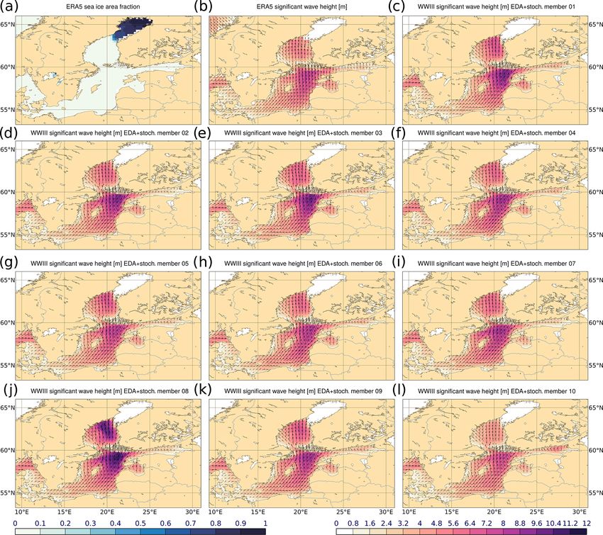
356                                       R. D. Osinski and H. Radtke: Ensemble hindcasting of wind and wave conditions

forecast runs from the same model for the same time in-                Some regional reanalysis (ensemble) datasets are already
stance but started at different initialization times, which is      freely available. Such regional reanalyses are produced, for
called a lagged-average forecast (LAF) ensemble (Hoffman            example, in the framework of the project “Uncertainties in
and Kalnay, 1983). A limitation here is also the number of          Ensembles of Regional ReAnalysis” (UERRA).1 At the mo-
forecasts covering the same time instance and the fact that a       ment, the ensemble datasets in this project are limited in their
newer forecast can be expected to have on average a better          temporal coverage or spatial resolution. It can be advanta-
forecast skill than a forecast at long lead times. The third        geous to be able to produce hindcasts of events whose spatio-
method is the utilization of a single model and applying            temporal resolution is adapted to the requirements defined by
perturbations to the initial conditions and/or to the model         a research objective. It has to be mentioned that the quality
physics.                                                            of a freely running hindcast can be expected to be inferior to
   Such an approach is used operationally at the European           such a (re)analysis product containing state-of-the art data as-
Centre for Medium-Range Weather Forecasts (ECMWF)                   similation techniques. Another database from which ensem-
since 1992. Initial conditions are perturbed by singular vec-       ble forecasts of local area models are available is from the
tors (Buizza, 1998), by a combination of ensemble data as-          Tigge-LAM archive (Swinbank et al., 2016).2 The available
similation (Buizza et al., 2008) with singular vectors or by        forecast models cover also only short periods and they are
breeding vectors (Toth and Kalnay, 1997) like in the case of        operational, meaning that the datasets are not homogeneous,
the National Centers for Environmental Prediction (NCEP).           because the model version can change during time.
Stochastic perturbations like stochastically perturbed param-          The Baltic Sea, which is a marginal sea in the north-east
eterization tendencies (SPPT) (Buizza et al., 1999), stochas-       of Europe, is taken as an example for the application of
tically perturbed parameterizations (SPP) (Ollinaho et al.,         the demonstrated procedure to produce ensemble hindcasts
2017) and stochastic kinetic energy backscatter (SKEB)              of wind and wave conditions by driving the WAVEWATCH
(Shutts, 2005) are used to perturb the model physics (Leut-         III® wave model with wind data produced with the WRF
becher et al., 2016, 2017). SPPT perturbs the model param-          ensemble model. Observed wave heights in this region do
eterizations by applying a multiplicative noise, and SKEB           not exceed 8.2 m (Björkqvist et al., 2017), and waves are
simulates the upscale transfer of kinetic energy from smaller       dominated by the wind sea (Broman et al., 2006; Soomere
to larger scales. Besides the application of SPPT in the global     et al., 2012). More detailed information about the Baltic Sea
ECMWF medium-range ensemble system, stochastic pertur-              wave climate for specific subregions is provided, for exam-
bations are also used in local area models (e.g. Bouttier et al.,   ple, by Björkqvist et al. (2017), Soomere (2005), Soomere
2012) and in ocean models like in NEMO (e.g. Brankart               et al. (2008) and Tuomi et al. (2011, 2014). As ERA5 is a
et al., 2015).                                                      global reanalysis, the demonstrated procedure is also appli-
   In a well-constructed ensemble, the ensemble spread re-          cable in other regions.
flects the average forecast error. Stochastic perturbations            The idea behind this study is to generate an ensemble hind-
need some time until a reasonable spread develops. Ensem-           cast on an event basis in a comparable way to operational
ble data assimilation (EDA) gives different estimations of the      weather forecasts by driving WRF with ERA5 including the
initial state representing its uncertainty. A forecast started      initial conditions from the ERA5 EDA with stochastic pertur-
from the different members develops the desired ensemble            bations (SKEB and SPPT). Other ensemble generation tech-
spread faster.                                                      niques are tested for comparison. The atmospheric data from
   ERA5 (Copernicus Climate Change Service, 2017) is the            a hindcast or forecast are discrete in time and space. This
newest global reanalysis from ECMWF. The resolution is rel-         limits the accuracy and affects the outcome if driving another
atively high with about 31 km resolution for the atmospheric        model like an ocean or wave model. This uncertainty is in-
variables, but, depending on the application, it can be still       vestigated by driving the wave model with different spatio-
too coarse. From ERA5, in contrast to previous reanalyses,          temporal resolutions.
an uncertainty measure based on an ensemble of data assim-
ilation is available.
   The Weather Research and Forecasting (WRF) (Ska-
marock et al., 2019) model is widely used in research as well
as in operational weather forecasting and includes implemen-
tations of the mentioned stochastic perturbation schemes.
The motivation of driving WRF with this new dataset is to
be able to produce hindcasts of atmospheric conditions in
different spatio-temporal resolutions including a measure of
uncertainty based on ensemble techniques. This allows us to
study, for example, the effect of the model resolution on ef-          1 http://www.uerra.eu/ (last access: 10 March 2020)
fects like upwelling and downwelling in coastal regions.               2 https://apps.ecmwf.int/datasets/history/tigge-lam-prod/   (last
                                                                    access: 10 March 2020)

Ocean Sci., 16, 355–371, 2020                                                                     www.ocean-sci.net/16/355/2020/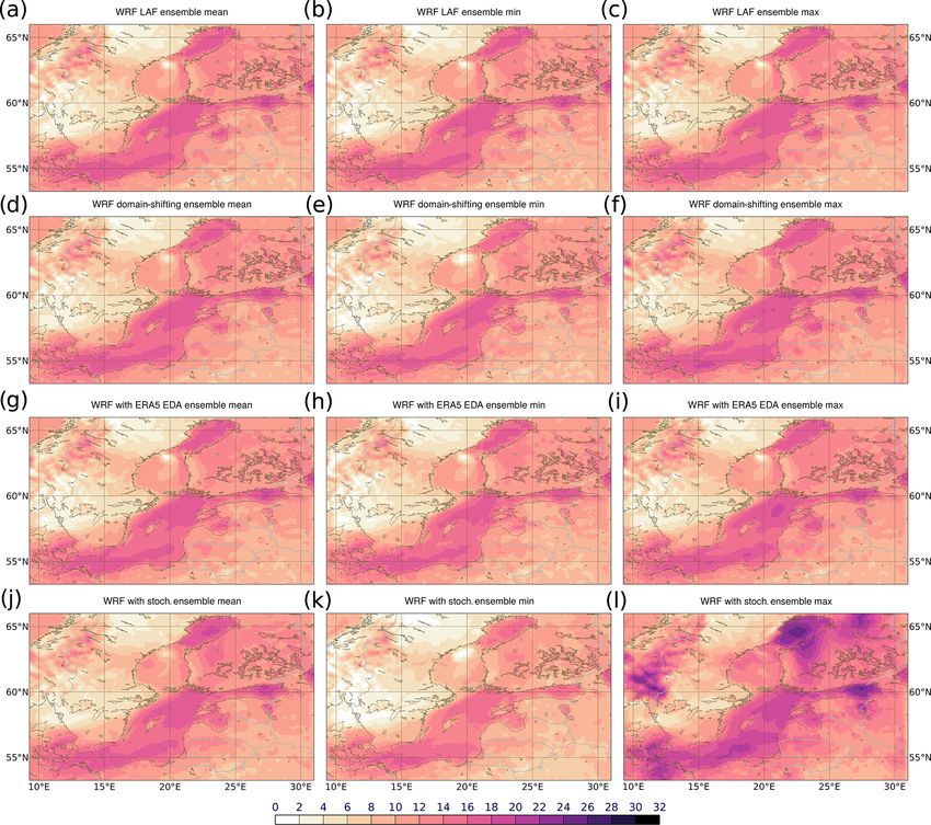
R. D. Osinski and H. Radtke: Ensemble hindcasting of wind and wave conditions                                                           357

2     Data and models                                                       tional observations (synoptic stations, ships, drifting buoys,
                                                                            aircraft observations and radio soundings). Large scales from
2.1     Data                                                                ERA40 and ERA-Interim are introduced into the data assim-
                                                                            ilation by large-scale mixing. The available period extends
2.1.1    ERA5                                                               back until 1961. To create an hourly dataset, the analysis
                                                                            fields were combined with the forecast lead times +1 to +5 h
ERA5 (Copernicus Climate Change Service, 2017)3 is the                      (retrieved from ECMWF).7 Wind data were interpolated bi-
follow-up ECMWF reanalysis of ERA-Interim produced                          linearly onto the regular wave model grid for the Baltic Sea
with the Integrated Forecasting System (IFS) cycle 41R2,4                   and described in the next section. This dataset was mainly
operationally at ECMWF in March 2016. It is provided un-                    used to produce a restart file for the wave model runs and for
der the Copernicus licence,5 allowing also commercial ap-                   calibration and validation of the wave model.
plications. Hourly reanalysis in about 31 km (∼ 0.28◦ )6 hor-
izontal resolution and 137 vertical model levels are avail-                 2.2     Models
able from 1979 (eventually 1950), and the dataset is getting
prolongated into the future with a delay of about 3 months.                 2.2.1    Atmospheric Weather Research and Forecasting
A state-of-the-art data assimilation technique is used (4D-                          model (WRF)
Var). In addition to the reanalysis, on a three-hourly basis, 10
members of an ensemble of data assimilation (EDA) are pro-                  The Weather Research and Forecasting model, WRF v4.0.3,8
vided as an uncertainty measure with half of the resolution                 in the Advanced Research WRF (ARW) version (Skamarock
of the reanalysis. The reanalysis data of surface fields and                et al., 2019) is applied here. It is used in non-hydrostatic
the 137 model levels that were extracted on an hourly basis                 mode in 0.126◦ horizontal resolution, and the model output
were interpolated onto a slightly higher 0.25◦ resolution grid              interval is 15 min. To investigate the dependence of the so-
for the period 21 until 24 February 2002 as recommended by                  lution of the wave model on the spatial and temporal reso-
ECMWF. ERA5 data from the ensemble of data assimilation                     lutions of the wind data, runs in 0.252 and 0.063◦ were pro-
were also interpolated bilinearly onto the same 0.25◦ regular               duced as well as output at a temporal resolution of 5 min. In
longitude–latitude grid.                                                    this way, a factor of about 4.5 between the highest WRF res-
   ERA5 also includes fields from the ECWAM wave model                      olution and the driving ERA5 fields is given, and the same
(ECMWF, 2016) in 0.36 and 1◦ spatial resolutions from the                   factor is between the ERA5 EDA fields and the WRF ensem-
ensemble of data assimilation. ERA5 is used for the initial                 ble runs. The domain is slightly larger than the Baltic Sea for
and lateral boundary conditions for the atmospheric hind-                   all runs. For the model configuration, the CONUS physics
casts with the WRF model. Lateral boundary conditions for                   suite (Wang et al., 2019) is used. This is a combination of
the Baltic Sea WAVEWATCH III® setup originate from a                        model physics adapted for the Continental United States of
setup for the North Sea. This coarser model is driven by                    America. As it is well tested, this physics setup is taken as it
ERA5 winds. ERA5 reanalysis and EDA wind and wave data                      is, and we assume that it should be reasonable for other re-
are used for comparison of the hindcasts produced with WRF                  gions in the mid-latitudes. The 89 vertical eta layers used in
and WAVEWATCH III® .                                                        this WRF setup, a specific vertical coordinate system in at-
                                                                            mospheric models, are adapted to be comparable to layer 2 to
2.1.2    UERRA/HARMONIE-v1                                                  90 of the IFS9 until 50 hPa. As initial conditions come from
                                                                            a different and coarser model, it needs some time until fine
The UERRA/HARMONIE-v1 dataset (Ridal et al., 2017)                          structures develop. Methods for spin-up reduction like digi-
contains analyses at 00:00, 06:00, 12:00 and 18:00 UTC as                   tal filter initialization (Peckham et al., 2016) have not been
well as hourly forecasts for +1 h until +6 h and thereafter                 tested. Instead, the WRF output is only used 12 h after ini-
three-hourly until 30 h. The HARMONIE model is used for                     tialization to drive the wave model. Neither data assimilation
the production of this dataset in about 11 km horizontal reso-              nor observation nudging is used. Hindcasts are produced in
lution, and the 3D-Var data assimilation is used with conven-               this study in a comparable way to a forecast, which is only
                                                                            downscaled from a global forecast model. For this reason,
    3 https://confluence.ecmwf.int/display/CKB/ERA5:+data+                  the results of this study are valid for both hindcasts and such
documentation (last access: 10 March 2020)                                  forecasts. The WRF Preprocessing System (WPS) in version
    4 https://www.ecmwf.int/en/forecasts/
documentation-and-support/changes-ecmwf-model/                                 7 https://apps.ecmwf.int/datasets/data/uerra (last     access:
ifs-documentation (last access: 10 March 2020)                              10 March 2020)
    5 http://apps.ecmwf.int/datasets/licences/copernicus/ (last ac-            8 https://github.com/wrf-model/WRF/releases    (last   access:
cess: 10 March 2020)                                                        10 March 2020)
    6 Grid cells in the Baltic Sea region have quite large aspect ratios;      9 https://www.ecmwf.int/en/forecasts/
the length of their sides in N–S direction can be roughly twice as          documentation-and-support/137-model-levels      (last     access:
long as in the E–W directions.                                              10 March 2020)

www.ocean-sci.net/16/355/2020/                                                                             Ocean Sci., 16, 355–371, 2020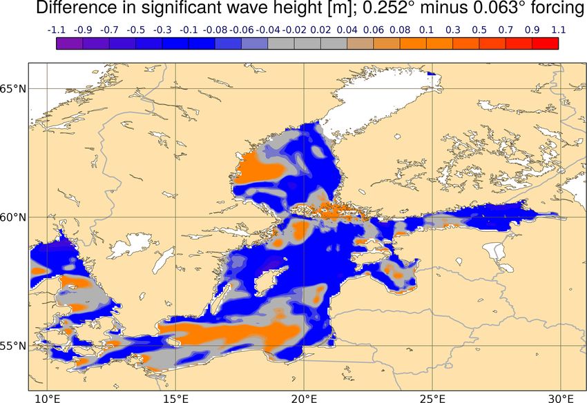
358                                      R. D. Osinski and H. Radtke: Ensemble hindcasting of wind and wave conditions

4.0.3 is used to prepare the input data for the model together    This includes wind input and dissipation after Ardhuin et al.
with the WPS V4 Geographical Static Data.10                       (2010) and the SHOWEX bottom friction scheme (Ardhuin
                                                                  et al., 2003). A sediment map based on the European Ma-
2.2.2   Wave model WAVEWATCH III®                                 rine Observation and Data Network (EMODnet)14 data was
                                                                  used for applying non-homogeneous bottom friction. The
WAVEWATCH III® v6.07 (Tolman, 1991; The WAVE-                     model runs were produced between 22 February 00:00 UTC
WATCH III® Development Group (WW3DG), 2019)11 is                  and 24 February 2002 00:00 UTC. WAVEWATCH III® was
used in this study for the Baltic Sea. It is a state-of-the art   started from initial conditions from a previous run conducted
third-generation wave model which is also used as an oper-        for 21 d and driven with UERRA/HARMONIE-v1. The sea
ational wave forecast model. A one-way nesting approach           ice area fraction is taken from ERA5. In the atmospheric
is applied (see Fig. 1): a setup with 0.1◦ resolution cov-        model, the stochastic perturbations of the model physics con-
ering the North Sea and a small part of the eastern At-           tribute significantly to the ensemble spread. Wave models
lantic Ocean is used to produce boundary conditions for the       include different source terms (e.g. wave generation, dissi-
Baltic Sea setup at the border with the North Sea. This is        pation, bottom-friction and so on), which are partly simpli-
not really necessary for the central and northern regions of      fied to make the model computationally more efficient or
the Baltic Sea, as very little wave energy passes the Dan-        are described empirically (Farina, 2002; Yildirim and Kar-
ish straits. To avoid showing unrealistic values in a part        niadakis, 2015). Nevertheless, the wave model ensemble ap-
of the domain, the nesting procedure was nevertheless ap-         proach here is based solely on the ensemble of the atmo-
plied. The GEBCO_2014 Grid in version 20150318 is used            spheric forcing data and includes no perturbations of the
as bathymetry.12 The Baltic Sea setup has a resolution of         source terms.
1 nmi (nautical mile) with 149.282 sea grid points, and the
bathymetry is based on the work of Seifert et al. (2001).
UERRA/HARMONIE-v1 was used for calibration and vali-              3     Ensemble hindcasts
dation of the setup against 1 month of data from buoys avail-
able from the Copernicus Marine Environment Monitoring            3.1    Wind fields
Service (CMEMS)13 with the previous WAVEWATCH III®
v5.16 version. A calibration and validation with the WRF          Six different approaches to generate an ensemble hindcast
forcing was not possible because of the short period that         are presented in this section (see Table 1). The first approach
has been hindcasted until now. Nevertheless, the wave model       is to generate an LAF ensemble. This is done by initializing
shows a satisfactory performance with the WRF forcing. De-        the WRF model at different times on 21 February 2002 at
tailed information about the calibration and validation pro-      every hour between 08:00 and 16:00 UTC, which results in
cedure of the wave model can be found in the Supplement.          nine runs covering the period from 22 to 24 February 2002.
Twenty-four directions starting at 7.5◦ with a 15◦ direction      The second approach is based on the domain shifting pre-
increment and 30 frequencies starting at 0.03453 Hz geomet-       sented by Pardowitz et al. (2016). The ERA5 reanalysis is for
rically distributed with a step of 1.1 are used for the dis-      this purpose shifted by one grid cell (0.25◦ ) in each direction
cretization of the energy spectrum. This is comparable to the     horizontally producing eight perturbed ensemble members.
settings for the wave model in ERA5. Soomere (2005) pro-          For the third approach, WRF is initialized from the ERA5
poses a finer resolution of the energy spectrum. This finer       fields from the ensemble of data assimilation. These fields
resolution was tested and the result is demonstrated in the       have a coarser resolution, but they are used in this study as
Supplement. A clear impact on the extreme wave heights is         the ERA5 reanalysis in 0.25◦ . This has the disadvantage that
visible, but it prolongs significantly the computing time. For    finer scales are not represented, but this is comparable to a
our specific application, the ERA5 discretization is a good       downscaling from a global ensemble model, except that the
compromise between computational effort and model perfor-         reanalysis is used here as lateral boundary condition (LBC).
mance. The physics packages are defined before compiling          As an alternative to keep the finer scales, it was tested to
the model by a so-called switch file. The switch file Ifre-       add perturbations to the initial fields, calculated by the differ-
mer1, provided with the model code, is applied in this study.     ence between the ERA5 EDA members and the EDA ensem-
  10 http://www2.mmm.ucar.edu/wrf/src/wps_files/geog_high_        ble mean, once with positive and negative sign to the ERA5
                                                                  HRES (high resolution) reanalysis. We did not find an im-
res_mandatory.tar.gz (last access: 10 March 2020)
  11 https://github.com/NOAA-EMC/WW3              (last access:
                                                                  provement against the direct application of the ERA5 EDA
10 March 2020)                                                    fields. SKEB and SPPT are used for the fourth approach and
  12 http://www.gebco.net (last access: 10 March 2020)            the fifth approach combines approaches three and four. For
  13 http://marine.copernicus.eu/services-portfolio/              approach six, the same setup is used as in approach five, but,
access-to-products/?option=com_csw&view=details&product_          as the ERA5 EDA fields are available every 3 h, runs 3 h ear-
id=INSITU_BAL_NRT_OBSERVATIONS_013_032 (last access:
10 March 2020)                                                        14 http://www.emodnet-geology.eu/ (last access: 10 March 2020)

Ocean Sci., 16, 355–371, 2020                                                                   www.ocean-sci.net/16/355/2020/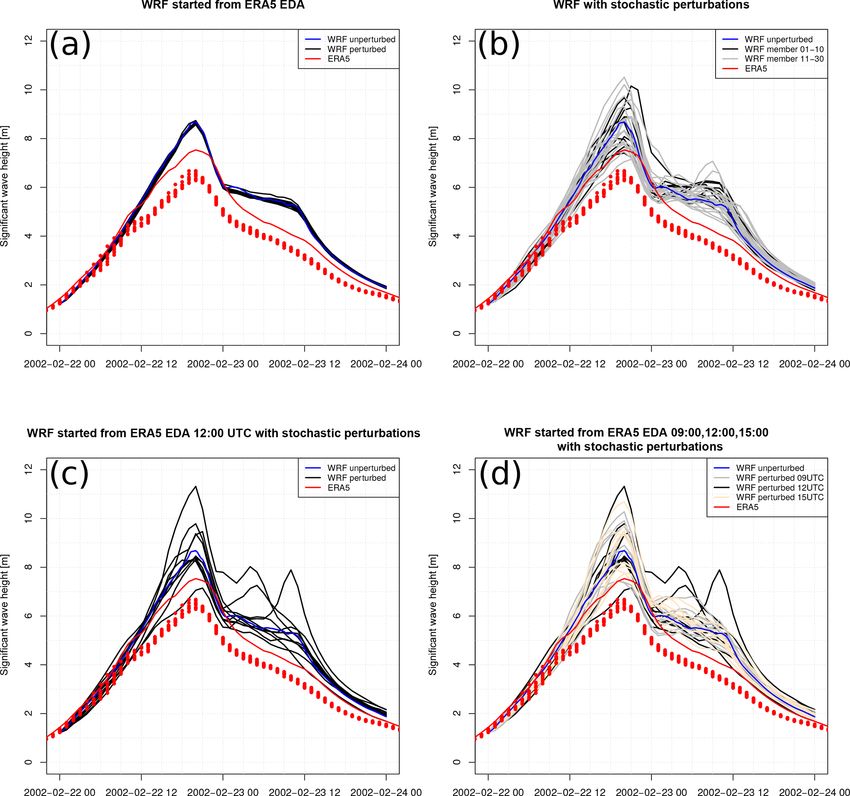
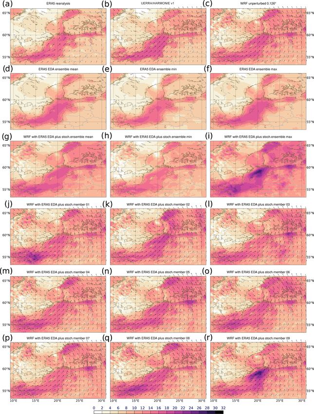
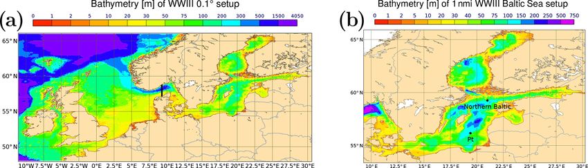
R. D. Osinski and H. Radtke: Ensemble hindcasting of wind and wave conditions                                                          359

Figure 1. Bathymetries (m) and domains of (a) 0.1◦ and (b) 1 nmi (nautical mile) WAVEWATCH III® setups; in black in the left panel,
(a) grid cells for the nesting of the Baltic Sea model are shown. The black point “Pt” in the right panel (b) shows the location of the time
series in Fig. 2, and the black point “Northern Baltic” is the location of the time series in Fig. 6.

lier and later are additionally used as in an LAF approach.             ditional information from the finer scales and resolves the
This leads to a 30-member ensemble.                                     orography, coastlines and islands better.
   In an ensemble system, it is important that the ensemble                 All ensemble techniques lead to deviations from the unper-
spread reflects the uncertainty. If the spread is too narrow,           turbed run. The LAF ensemble shows a very small spread.
the system is “underdispersive”, meaning that the forecast is           In fact, this is good, because it means that irrespective of
overconfident and vice versa for an “overdispersive” or “un-            the starting time of the WRF model being shifted by a few
derconfident” forecast. One tool for quantifying the quality            hours the outcome is comparable. The first three approaches
of the ensemble spread is, for example, the Talagrand (rank)            show a lower ensemble spread than the ensembles which in-
diagram (Hamill, 2001), and there are other quality measures            clude stochastic perturbations. Compared to the ERA5 EDA
like, for example, reliability, resolution, accuracy or sharp-          members, it demonstrates that these ensembles are underdis-
ness, which are important for a good ensemble system (Mur-              persive. The uncertainty is underestimated by applying these
phy and Winkler, 1992). To be able to use the traditional en-           approaches. During the first hours of the ensemble with only
semble verification methods (Jolliffe and Stephenson, 2003),            stochastic perturbations (ensemble approach four), all mem-
long time series are needed, which could not be produced in             bers are identical, as it needs some time until the perturba-
this study. For this reason, an absolute statement on which of          tions introduce spread. Starting from the ERA5 ensemble of
the tested approaches performs best cannot be given based on            data assimilation (ensemble approaches 3, 5 and 6), spread
only one single hindcasted event. The different approaches              is visible from initialization on. Even with the coarser res-
are compared against the ERA5 reanalysis and the ERA5                   olution of these fields, its application seems to be working,
members from the ensemble of data assimilation. As a larger             but additionally stochastic perturbations are necessary to pro-
variability can be expected in the higher-resolution model, it          duce a larger spread. The WRF ensemble started from ERA5
can be assumed that it increases also the uncertainty, which            EDA fields at 09:00, 12:00 and 15:00 UTC and also rep-
should be reflected by a larger spread than found in the much           resents the uncertainty at 21 February 2002 at 21:00 UTC,
coarser data from the ERA5 ensemble of data assimilation.               where the lowest values in the ERA5 EDA members (Fig. 2)
   A good agreement at a specific location between the                  in the shown period can be found. With only stochastic per-
ERA5 reanalysis and the WRF runs is visible during the                  turbations, such low values are also visible, but a few hours
first 20 h in Fig. 2. The wind speed maximum is higher                  too early. For the last simulation day, the spread of the com-
than in ERA5. For comparison, the closest grid cell of the              bined ERA5 EDA and stochastic perturbations approach is
UERRA/HARMONIE-v1 data is plotted and also shows                        very large, but it could not be tested if it is overdispersive.
higher values than ERA5. From ERA5, also the wind speed                     Spatially (Fig. 3), the spread in the WRF ensemble started
from the closest grid cell of the 0.25◦ grid is plotted. The            from ERA5 EDA is very small. A much larger spatial vari-
initial conditions were prepared with the WRF preprocess-               ability appears by applying stochastic perturbations. Espe-
ing system and can have slightly different values from taking           cially strong wind is present in some members over the north-
simply the closest grid cell. The resolution of the WRF runs            ern part of the Baltic Sea. The LAF approach also shows very
is closer to the one from UERRA/HARMONIE-v1, and a                      little spread spatially over the entire domain. Domain shift-
stronger variability and also higher extremes can be expected           ing also did not produce as strong a variability as applying
due to the difference in the ERA5 resolution. WRF adds ad-              stochastic perturbations (Fig. 3). The combination of ERA5

www.ocean-sci.net/16/355/2020/                                                                           Ocean Sci., 16, 355–371, 2020
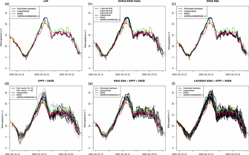
360                                          R. D. Osinski and H. Radtke: Ensemble hindcasting of wind and wave conditions

Table 1. Methods tested for the generation of an ensemble hindcast with WRF.

   Approach     Procedure                                                                                                   No. of members
   1            LAF approach, WRF initialized at different times (21 February 2002 between 08:00 and 16:00 UTC)                            9
   2            Domain-shifting approach, ERA5 shifted horizontally by one grid cell                                                       8
   3            ERA5 EDA fields used for initial conditions                                                                               10
   4            Stochastic perturbations (SKEB and SPPT) together with random perturbations of LBCs                                       10
   5            As approach four but initialized from ERA5 EDA as in approach 3                                                           10
   6            As approach five but additional runs started at 3 h earlier and later                                                     30

Figure 2. Time series demonstrating the simulation results of the different ensemble generation strategies at one specific location: (a) lagged-
average forecast (LAF) ensemble (Hoffman and Kalnay, 1983), (b) domain shifting (Pardowitz et al., 2016), (c) WRF runs started from 10
ERA5 4D-EnVAR members with HRES LBCs, (d) stochastic perturbations (SPPT and SKEB) (Buizza et al., 1999; Shutts, 2005), (e) ERA5
4D-EnVAR as starting conditions plus stochastic perturbations, and (d) LAF started from ERA5 4D-EnVAR at 09:00, 12:00 and 15:00 UTC
plus stochastic perturbations; results shown for 56.17◦ N, 19.39◦ E.

EDA and stochastic perturbations produces members which                   and 30 members. The spread is in this case larger but still
show a strong variability in the central Baltic Sea (Fig. 4).             inferior to the 30-member approach number six with ERA5
   A strong variability in the northern Baltic Sea as well as in          EDA as initial conditions and stochastic perturbations. Also
the central Baltic Sea is present by initializing WRF at 09:00,           the region in the central Baltic Sea gains spread by adding
12:00 and 15:00 UTC from ERA5 EDA fields with stochastic                  additional members, but it contains a lower spread than in ap-
perturbations. Ten members are a small number to sample the               proach six shown in Fig. 5. This demonstrates that 10 mem-
uncertainty.                                                              bers might be still insufficient to sample the entire range of
   Comparing a 10- with a 30-member ensemble is not re-                   uncertainty and that the combined application of model and
ally a fair comparison, as a too small ensemble size leads to             initial perturbations is beneficial to create a larger spread.
an undersampling of the uncertainty. Ensemble approach six
shows in the ensemble maximum high values in the central as
well as in the northern part of the Baltic Sea. Figure 2 shows
also the WRF ensemble with only stochastic perturbations

Ocean Sci., 16, 355–371, 2020                                                                            www.ocean-sci.net/16/355/2020/
R. D. Osinski and H. Radtke: Ensemble hindcasting of wind and wave conditions                                                         361

Figure 3. Ensemble mean (a, d, g, j), minimum (b, e, h, k) and maximum (c, f, i, l) wind speed (m s−1 ) of WRF ensemble based on LAF
approach (a–c), domain shifting (d–f), initial conditions from the ERA5 EDA (g–i) and on stochastic perturbations (j–l). All initialized at
21 February 2002 12:00 UTC. Shown are results for 23 February 2002 09:00 UTC.

3.2   Wave fields                                                       a much higher resolution with 1 nmi compared to the 0.36◦
                                                                        ECWAM model of the ERA5 reanalysis, and the WRF wind
                                                                        forcing is spatially (0.126◦ vs. 0.28◦ ) and temporally (150
The LAF and domain-shifting approaches were not used to                 vs. 600 ) of higher resolution. This can explain locally much
drive the wave model, because they show a relatively small              higher values and a stronger variability. Especially the max-
spread. Figure 6 shows a time series at a location in the cen-          imum of the (wind speed and the) significant wave height
tral Baltic Sea (see Fig. 1). The comparison with the closest           varies strongly between the different ensemble realizations.
grid cell from ERA5 shows a good agreement in the temporal              Differences in the wave fields of the ensemble members can
evolution of growth and a comparable trend in the decay of              be due to a different dynamical evolution of the storm or due
the significant wave height, but the maximum peak is about              to different tracks in the atmospheric model members (com-
1 m lower in ERA5. ERA5 also shows the second peak only                 pare Osinski et al., 2016). Already a slight change in the track
very weakly and some hours later during the middle of the               of the storm can provoke large differences in the maximum if
second simulation day. WAVEWATCH III® in this study has

www.ocean-sci.net/16/355/2020/                                                                          Ocean Sci., 16, 355–371, 2020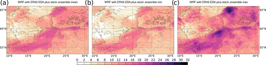
362                                     R. D. Osinski and H. Radtke: Ensemble hindcasting of wind and wave conditions

Figure 4. WRF ensemble approach number five generated by starting the 10 members from 10 ERA5 EDA members at 21 February 2002
12:00 UTC plus stochastic perturbations SPPT and SKEB. Shown are results for 23 February 2002 09:00 UTC. (a) The ERA5 reanalysis;
(d) ERA5 EDA ensemble mean, (e) minimum, and (f) maximum; (c) WRF unperturbed; (g) WRF ensemble mean, (h) minimum, and
(i) maximum; (b) UERRA/HARMONIE-v1; and (j–r) nine perturbed WRF members are shown. Wind speed (m s−1 ) and direction are
shown as arrows.

Ocean Sci., 16, 355–371, 2020                                                                 www.ocean-sci.net/16/355/2020/
R. D. Osinski and H. Radtke: Ensemble hindcasting of wind and wave conditions                                                  363

Figure 5. Ensemble mean (a), minimum (b) and maximum (c) wind speed (m s−1 ) from WRF ensemble approach number six generated by
starting three times 10 members from ERA5 EDA members at 21 February 2002 09:00, 12:00 and 15:00 UTC plus stochastic perturbations
SPPT and SKEB. Shown are results for the 23 February 2002 09:00 UTC.

looking at a specific location in such a high resolution. With     Toini and Rafael, with the highest observed significant wave
0.36◦ resolution in ERA5, a slight change in the track can be      heights discussed by Björkqvist et al. (2017) were addition-
assumed to not lead to such strong differences.                    ally hindcasted and are presented in the Supplement. They
   Figure 7 shows the different wave model members driven          seem to be less sensitive on the perturbations. Based on the
by WRF with ERA5 EDA initial conditions and stochastic             short time series of observations, it is difficult to judge which
perturbations. All members show high values in the cen-            significant wave height is still realistic.
tral Baltic Sea. The time series shown in Fig. 6 represents           A shortcoming of the presented procedure can be that the
the highest significant wave height on 22 February 2002 at         wave model runs were all started from the same initial state.
09:00 UTC. There is also a strong variability between the          This means that a certain time is needed until the different
different ensemble members in this region. Wave heights in         members diverge, especially as the total wave height is a
member 08 are especially higher than in the other members          combination of wind sea and swell. The latter needs some
in the Gulf of Bothnia, but this member shows also much            time to travel, so regions which are predominated by swell
higher wave heights than the other members in the central          can be assumed to need a longer period to produce a reason-
Baltic Sea. In the western Baltic Sea the differences between      able spread with this setting. For the Baltic Sea, events with
the members are not that strong. The overall spatial pattern of    a strong influence of swell are infrequent (e.g. Broman et al.,
the significant wave height looks similar between ERA5 and         2006; Soomere et al., 2012). French Guiana, for example, is
WRF ensemble members. The wave models (Fig. 6) driven              one region which is swell dominated. Osinski et al. (2018)
by the WRF ensemble hindcast started from the ERA5 EDA             estimated the 100-year return level of the significant wave
initial conditions show a very small spread. A difference can      height of northerly swell events at the French Guiana coast.
be especially seen at the second peak. Much stronger differ-       Such events are generated in the North Atlantic and travel
ences are provoked by the WRF ensemble based on stochas-           until the north-eastern coast of South America. For hindcast-
tic perturbations. Combining both ERA5 EDA fields as initial       ing such events with the demonstrated procedure, a large do-
conditions and stochastic perturbations produces a spread of       main would be necessary and long lasting forecast horizons,
a similar size. The simulated significant wave heights of the      so that the waves are already perturbed where generated and
most extreme members with about 11.2 m are clearly above           over their lifetime as well. This can lead to stronger devia-
the highest observations with about 8.2 m (Björkqvist et al.,      tions from the real past state.
2017). One reason could be an overdispersion of the wind
fields of the WRF ensemble. The stochastic perturbations           3.3   Robustness of the ensemble spread depending on
were not calibrated, as a larger number of hindcasted events             the ensemble size
are necessary to be able to optimize the perturbations. An-
other issue is the roughness length of the sea surface, which      Each ensemble member is a random draw of the probability
is defined as a constant value in the applied WRF setup. Un-       density function (PDF) of the forecast/hindcast uncertainty.
der severe storm conditions, the roughness of the sea surface      In the extreme case of having only two members, it is very
should increase, resulting in a reduction of atmospheric ki-       unlikely that the most extreme cases are represented. By in-
netic energy and a corresponding limitation of wave growth.        creasing the ensemble size, the probability is getting higher
An investigation of the impact of the constant roughness of        that the full range of uncertainty is sampled. For local area
the sea surface on the wave height was out of the scope of         models, operational weather forecast centres produce ensem-
this study. This effect could lead to a systematic overestima-     bles with around 10 to 20 members. At first sight, this num-
tion of the wave heights in some storms. The storm events,         ber seems to be comparable to the presented study. If driv-

www.ocean-sci.net/16/355/2020/                                                                    Ocean Sci., 16, 355–371, 2020
364                                       R. D. Osinski and H. Radtke: Ensemble hindcasting of wind and wave conditions

Figure 6. Significant wave height (m) at station Northern Baltic (59.25◦ N, 21.00◦ E; see Fig. 1), driven by the WRF ensemble based on
(a) initializations at 21 February 2002 12:00 UTC from ERA5 EDA, (b) ERA5 reanalysis and stochastic perturbations, (c) ERA5 EDA with
SKEB and SPPT, and (d) ERA5 EDA with SKEB and SPPT initialized additionally on same day at 09:00 and 15:00 UTC; ERA5 significant
wave heights from the ECWAM model in 0.36◦ resolution; Shown are results for 22 February 2002 21:00 UTC.

ing the regional model from a global ensemble with about             model. To get an idea of how many ensemble members are
30 to 50 ensemble members, one can use a clustering tech-            reasonable in this case, 500 members have been generated
nique to identify the most representative members instead of         with stochastic perturbations. From these 500 members, an
randomly selecting a small subsample, which improves the             ensemble with N members is generated, with N starting at
ensemble performance (e.g. Nuissier et al., 2012). If the en-        10 and increasing until 300. Ten million samples of each en-
semble is initialized several times per day, the different runs      semble of size N are selected by randomly choosing N out
can be combined using the LAF approach (e.g. Raynaud and             of the 500 members. The standard deviation is used as a mea-
Bouttier, 2017). To predict the probability of the exceedance        sure for the ensemble spread and is calculated for each of the
of a certain threshold, one can apply also neighbourhood             10 million samples of the ensemble of size N. The number
techniques (e.g. Theis et al., 2005) or post-processing tech-        of possible combinations of selecting N out of 500 members
niques like Bayesian Model Averaging (Raftery et al., 2005).         can be determined by using the binomial coefficient (500  N ).
Neither the initial and lateral boundary conditions that come        This number exceeds 10 million for all tested ensemble sizes
from a large ensemble in this study nor the application of           between 10 and 300. If the ensemble size is reasonable to
neighbourhood or other post-processing techniques helps,             get a robust estimate of the uncertainty, the spread should be
because the ensemble members are used to drive a wave                relatively similar between each of the samples.

Ocean Sci., 16, 355–371, 2020                                                                     www.ocean-sci.net/16/355/2020/
R. D. Osinski and H. Radtke: Ensemble hindcasting of wind and wave conditions                                                  365

Figure 7. (a) ERA5 sea ice area fraction (0–1); (b) ERA5 ECWAM significant wave height (m) with direction in meteorological conven-
tion and (c–l) 10 WAVEWATCH III® members driven by WRF ensemble initialized from 10 ERA5 EDA members at 21 February 2002
12:00 UTC with SPPT and SKEB. Shown are results for 22 February 2002 21:00 UTC.

   Figure 8 shows box-and-whisker plots for the 10 million          larger number of ensemble members is necessary to sam-
samples for ensemble sizes between 10 and 300 members.              ple the entire uncertainty range. With increasing ensemble
The variation of the spread in the 10 million samples 12 h          size, it is getting more probable that the entire uncertainty
after initialization is demonstrated in the left panel (Fig. 8a).   range is sampled. This is why the range of the box-and-
As it needs some time so that the stochastic perturbations          whisker plots is decreasing with increasing ensemble size. At
provoke spread between the ensemble members, there is a             22 February 2019 00:00 UTC, the uncertainty is lower and/or
lead time dependence in the spread. The right panel (Fig. 8b)       the spread as a measure of uncertainty is not yet fully devel-
presents a situation 25 h after initialization. At this time,       oped after 12 h. As the robustness of the ensemble spread
the wind speed is very high (see Fig. 2). In extreme situ-          seems to be dependent on the uncertainty, the range of the
ations, in which we are especially interested, we expect a          box-and-whisker plots is much inferior at 22 February 2019
higher uncertainty. This higher uncertainty is represented by       00:00 UTC than 13 h later. To achieve a general statement
a larger spread. All the ensembles with sizes between 15            about the ensemble size–spread relation, a much larger sam-
and 100 members show a median of the spread around one              ple over a longer period must be investigated, but it can al-
at 22 February 2019 13:00 UTC. The 10-member ensemble               ready be concluded that an ensemble size of only 10 ran-
has a slightly lower median. With a higher uncertainty, a           domly generated members, as demonstrated in this applica-

www.ocean-sci.net/16/355/2020/                                                                    Ocean Sci., 16, 355–371, 2020
366 R. D. Osinski and H. Radtke: Ensemble hindcasting of wind and wave conditions
Figure 8. Box-and-whisker plots of the standard deviation of the 10 m wind speed at 19.39◦ E, 56.17◦ N of 10 million samples of ensembles
of size 10 to 300 randomly sampled from an ensemble with 500 members generated with WRF by applying SKEB and SPPT; shown are
results for (a) 22 February 2002 00:00 and (b) 13:00 UTC (compare with Fig. 2).
tion, can lead to a significant overestimation or underesti- very close. The effect between the 60 min temporal resolu-
mation of the uncertainty. Depending on the application, the tion and a forcing in higher temporal resolution on the signif-
ensemble size needs to be selected as a compromise between icant wave height is relatively low with about 2 cm. System-
the robustness of the uncertainty estimate and the computa- atic differences cannot be found based on the small sample,
tional cost. but this sensitivity test indicates that the choice of the 15 min
resolution is a reasonable compromise between a good rep-
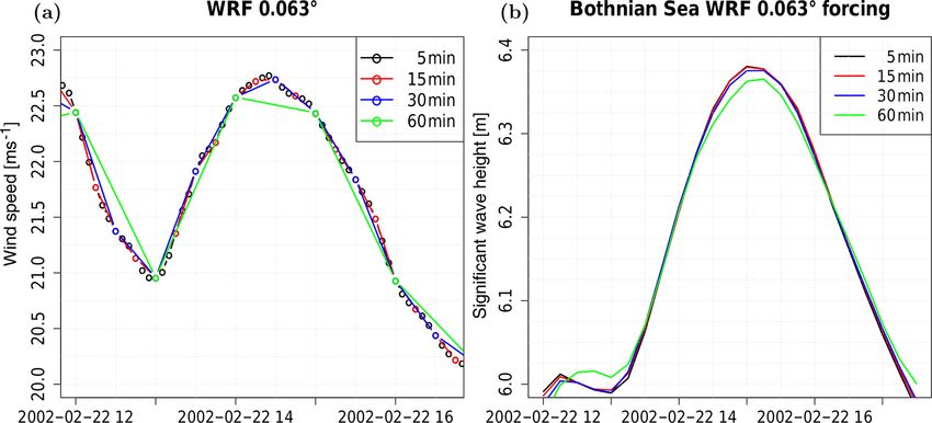
3.4 Impact of the spatio-temporal resolution of the resentation of the extreme values and file size.
atmospheric forcing on the significant wave height A stronger impact can be expected from the spatial resolu-
tion of the driving wind fields, because a coarser resolution
The numerical time step of a wave model is less than a minute of the atmospheric model can be assumed to produce lower
(typical for explicit numerical schemes) or few minutes (typ- extreme wind speeds as a grid cell represents the average
ical for implicit numerical schemes). The wave model there- value over the area it covers. By adapting, for example, the
fore needs updated wind information, e.g. every 30 s. This parameter BETAMAX, which describes the maximum value
is done by interpolation from the wind forcing that is pro- of wind–wave coupling, this difference can be compensated
vided, e.g. every hour or every third hour. A higher temporal for. A better representation of the complex coastline of the
resolution of atmospheric forcing data than 1 h is normally Baltic Sea as well as of the various islands is given by the
not available. If a variable in the ocean or wave model to be higher resolved WRF model. For this reason, a difference
driven has a short response time (e.g. surface current gen- in the spatial pattern of the significant wave height can be
erated by wind compared to sea surface temperature (SST) expected. A test with the coarsest (0.252◦ ) and the highest
whose response is slower), and the variability of the atmo- resolutions (0.063◦ ) produced in this study has been con-
spheric forcing in between the temporal resolution of the ducted. The same parameter sets were used, as a calibration is
forcing fields is high, the result can be an underestimation or not possible based on the short-period hindcasted with WRF.
overestimation and an erroneous time evolution. One imag- Figure 10 shows the difference between these two forcings
inable solution is to use maximum values during the output on one time step in the significant wave height.
time interval of the atmospheric model, but this can lead to One grid cell of the coarser WRF setup contains 16 grid
spatially inconsistent fields, especially if the time interval is cells of the high-resolution setup. Wave height maxima as
very long. To test the impact of different temporal resolutions well as minima were found to be more extreme in the higher
on the significant wave height, wind fields in 5 min resolu- resolution with a higher spatial variability. It would be in-
tion were produced with the 0.063◦ setup. Figure 9 shows teresting to determine the remaining difference in the wave
the wind field in 5, 15, 30 and 60 min resolutions at one spe- parameters provoked by the atmospheric forcings with dif-
cific grid cell and the resulting significant wave height at the ferent resolutions after a calibration of the wave model, done
same location and time. by applying an automatic and objective calibration procedure
It can be seen that the wind speed maximum in the 60 min like, for example, the one proposed by Gorman and Oliver
resolution is about 0.25 m s−1 below the maxima of the (2018). Tuomi et al. (2014) studied the effect of different
higher temporal resolutions. Between the higher temporal spatio-temporal resolutions of the wind forcing on a wave
resolutions of the wind data, the wind speed maxima are
Ocean Sci., 16, 355–371, 2020 www.ocean-sci.net/16/355/2020/R. D. Osinski and H. Radtke: Ensemble hindcasting of wind and wave conditions 367
Figure 9. (a) Wind speed (m s−1 ) in 0.063◦ setup and (b) significant wave height (m) at 61.8◦ N, 20.23◦ E; test case without sea ice.
Figure 10. Difference in the significant wave height (m) in WAVEWATCH III® between simulation driven by WRF with 0.252◦ and by
0.063◦ in 15 min temporal resolution at 22 February 2002 21:00 UTC. The northern part of the Gulf of Bothnia is covered by sea ice.
model with a higher spatial resolution than applied here. A then it was validated with this dataset and also with forc-
wave model with a higher resolution might benefit more from ing data produced with the atmospheric setup used in this
a higher resolution of the wind forcing. study, as demonstrated in the Supplement. A lagged-average
WRF forecast ensemble showed only little spread with initial
and lateral boundary conditions based entirely on the high-
4 Conclusions resolution ERA5 reanalysis fields. The spread of the LAF
ensemble cannot be easily adapted.15
Different approaches for hindcasting a single relatively
strong storm event in the Baltic Sea were tested in this 15 A weighting of the different realizations (in this case of the
study to create an ensemble hindcast of atmospheric (wind) wave model) by giving the runs more weight, which is expected to
and wave conditions based on a state-of-the-art atmospheric have a lower error, is possible. In this case more weight to the runs
mesoscale model and a third-generation wave model. The which have smaller errors in the verification of a large sample of
objective of the ensemble approach is a quantification of hindcasts should be given (e.g. more weight to runs with lower lead
the uncertainty of the hindcast. The wave model was cali- time to the desired event), but this can be expected to not strongly
brated based on a publicly available regional reanalysis, and enlarge the ensemble spread.
www.ocean-sci.net/16/355/2020/ Ocean Sci., 16, 355–371, 2020368 R. D. Osinski and H. Radtke: Ensemble hindcasting of wind and wave conditions
A domain-shifting approach with ERA5, in which the in- The robustness of the spread depending on the ensemble
put fields are shifted into all directions by one grid cell, size was tested by randomly generating ensembles with dif-
shows a more or less similar spread to the LAF ensemble, ferent sizes (10 to 300 members) from an ensemble hind-
with the same advantage of using the high-resolution reanal- cast with 500 members. For small ensembles, the range of
ysis data only. The number of ensemble members and the the ensemble spread can differ largely, depending on which
spread of the ensemble is limited to the number of reason- members were randomly selected. In operational services,
able shifts. Too large shifts can be expected to degrade the this problem is tackled by selecting, for example, already
hindcast.16 representative members from a larger global ensemble. To
Starting WRF from the ERA5 EDA members shows also achieve a comparable robust estimate of the uncertainty, the
a spread of similar size as with the two other approaches. ensemble size for the here-presented approach without pres-
The disadvantage is the coarser resolution of the initial fields. election of ensemble members must be larger than the one of
Fine-scale structures are not present in these fields so that the operational local area model ensembles.
ensemble spread is limited. Stochastic perturbations produce Another source of uncertainty arises from the spatio-
a much larger spread but need some time to develop. The first temporal discretization of the atmospheric model and the re-
12 h is not used in this study, because that period is assumed sulting forcing fields for the wave model. Errors introduced
to be affected by a model spin-up. This is not a shortcoming by a coarse temporal resolution of the driving wind fields in
for a hindcast procedure. the significant wave height are relatively small in this event
A combination of stochastic perturbations and an initial- test case. For a strong event with a significant wave height
ization from the ERA5 EDA fields produces also deviations of about 6.3 m, the difference in wave heights between simu-
from the unperturbed runs which are not present by only us- lations using 5 and 60 min temporally resolved wind forcing
ing the stochastic perturbations. This approach is especially is only of the order of 2 cm. Between 15 and 5 min tempo-
interesting and is close to what is used in meteorological ral resolution, the impact on the wave height is negligible for
weather forecast centres for the operational forecasts. The the demonstrated case. The horizontal resolution has a much
wind fields from this ensemble hindcast produce also a large stronger impact. This can potentially be corrected by cali-
spread in the wave model. A visual comparison with the brating the model to the different wind forcings. It would be
ERA5 wave model ensemble of data assimilations indicates interesting to estimate the remaining difference, but this was
that this spread is more reasonable than the one obtained us- not possible in the framework of this study as a calibration
ing the first three discussed ensemble generation approaches. of the models is not feasible based on a hindcast of only a
The peak of the significant wave height in the Baltic Proper single event.
of the most extreme members is, however, with about 11 m A combination of ERA5 EDA fields as initial conditions
strongly exceeding existing observations in this region. One and the stochastic perturbations showed the ability to pro-
possible reason could be an overdispersion of the ensemble duce a larger spread than with the other demonstrated ap-
system. Another important factor is the roughness of the sea proaches. Stochastic perturbations have not been tuned in this
surface and its impact on the dynamics of the storm. In the study. Producing longer time series, for tuning and validating
presented setup, the roughness length of the sea surface is the model, could lead to a reasonable measure of the hindcast
defined as a constant value. The constant sea surface rough- uncertainty on the regional scale.
ness could lead to systematic overestimations of the wind Operational atmospheric and wave products exist with
speed resulting in too high wave heights. A coupling of the a comparable or even higher resolution than applied here,
atmospheric model with the wave model would allow us to whose quality is superior to what can be reached with the
adapt the roughness length depending on the sea surface con- demonstrated procedure, as they include state-of-the-art data
ditions, and it can lead to a limitation of the wave growth. assimilation techniques. The application of such operational
products is, however, limited by the available periods and
also by the inhomogeneity of the datasets. The demonstrated
16 As the WRF model has a finer resolution, shifts different than approach allows us to adapt the spatio-temporal resolution
multiples of one grid cell by adding or subtracting an offset onto the and the ensemble size to specific research questions for
coordinates of the ERA5 grid would change the interpolation for the event-based hindcasts in a homogeneous manner over the en-
WRF initial and lateral boundary conditions. This was not tested, tire available ERA5 period.
and it was also not investigated systematically if members gener-
ated from smaller shifts are closer to the unperturbed run or if shifts
into a certain direction (e.g. into flow direction or perpendicular to
Code availability. The WRF source code is available from https://
it) lead to different spreads than shifts into other directions, which
github.com/wrf-model/WRF/releases (last access: 10 March 2020),
would mean that there are systematic differences between the mem-
and the WAVEWATCH III® source code is available from https:
bers to be taken into account by the interpretation of the ensemble
//github.com/NOAA-EMC/WW3 (last access: 10 March 2020).
data. A test with shifts of two and three grid cells into north, west,
south and east directions was performed, and it indicates that there
are systematic differences.
Ocean Sci., 16, 355–371, 2020 www.ocean-sci.net/16/355/2020/R. D. Osinski and H. Radtke: Ensemble hindcasting of wind and wave conditions 369
Data availability. ERA5 and the UERRA/HARMONIE- References
v1 reanalysis can be retrieved from the Climate Data
Store at https://cds.climate.copernicus.eu/cdsapp#!/dataset/ Ardhuin, F., H C Herbers, T., O’Reilly, W., and Jessen,
reanalysis-era5-single-levels?tab=overview (Copernicus Climate P.: Swell Transformation across the Continental Shelf.
Change Service, 2017) and https://cds.climate.copernicus.eu/ Part I: Attenuation and Directional Broadening, J.
cdsapp#!/dataset/reanalysis-uerra-europe-complete?tab=overview Phys. Oceanogr., 33, 1921, https://doi.org/10.1175/1520-
(Copernicus Climate Data Store, 2019). 0485(2003)0332.0.CO;2, 2003.
Ardhuin, F., Rogers, E., Babanin, A. V., Filipot, J.-F., Magne, R.,
Roland, A., van der Westhuysen, A., Queffeulou, P., Lefevre,
Sample availability. Ensemble hindcasts of wind and wave fields J.-M., Aouf, L., and Collard, F.: Semiempirical Dissipation
presented in this study can be requested by contacting the corre- Source Functions for Ocean Waves. Part I: Definition, Cal-
sponding author. ibration, and Validation, J. Phys. Oceanogr., 40, 1917–1941,
https://doi.org/10.1175/2010JPO4324.1, 2010.
Björkqvist, J.-V., Tuomi, L., Tollman, N., Kangas, A., Pettersson,
H., Marjamaa, R., Jokinen, H., and Fortelius, C.: Brief commu-
Supplement. The supplement related to this article is available on-
nication: Characteristic properties of extreme wave events ob-
line at: https://doi.org/10.5194/os-16-355-2020-supplement.
served in the northern Baltic Proper, Baltic Sea, Nat. Hazards
Earth Syst. Sci., 17, 1653–1658, https://doi.org/10.5194/nhess-
17-1653-2017, 2017.
Author contributions. RDO is responsible for the concept of this Bouttier, F., Vié, B., Nuissier, O., and Raynaud, L.: Impact of
study, prepared the configurations of WRF and WAVEWATCH Stochastic Physics in a Convection-Permitting Ensemble, Mon.
III® , conducted the simulations, and prepared the presentation of Weather Rev., 140, 3706–3721, https://doi.org/10.1175/MWR-
the results. HR was involved in the discussion of the results and in D-12-00031.1, 2012.
the preparation of the article. Brankart, J.-M., Candille, G., Garnier, F., Calone, C., Melet, A.,
Bouttier, P.-A., Brasseur, P., and Verron, J.: A generic approach
to explicit simulation of uncertainty in the NEMO ocean model,
Competing interests. The authors declare that they have no conflict Geosci. Model Dev., 8, 1285–1297, https://doi.org/10.5194/gmd-
of interest. 8-1285-2015, 2015.
Broman, B., Hammarklint, T., Kalev, R., Soomere, T., and Vald-
mann, A.: Trends and extremes of wave fields in the north-eastern
Acknowledgements. This study was financed by the BONUS MI- part of the Baltic Proper, Oceanologia, 48, 165–184, 2006.
CROPOLL project, which has received funding from BONUS (Art Buizza, R.: Impact of Horizontal Diffusion on
185), funded jointly by the EU and Baltic Sea national funding insti- T21, T42, and T63 Singular Vectors, J. Atmos.
tutions. For the calibration and validation of the Baltic Sea WAVE- Sci., 55, 1069–1083, https://doi.org/10.1175/1520-
WATCH III® setup, computing resources at the North German Su- 0469(1998)0552.0.CO;2, 1998.
percomputing Alliance (HLRN) were consumed and E.U. Coper- Buizza, R., Milleer, M., and Palmer, T. N.: Stochastic represen-
nicus Marine Service Information were used. The simulations in tation of model uncertainties in the ECMWF ensemble pre-
this study were generated using Copernicus Climate Change Ser- diction system, Q. J. Roy. Meteor. Soc., 125, 2887–2908,
vice information (2018/2019). The research and work leading to the https://doi.org/10.1002/qj.49712556006, 1999.
UERRA dataset used in this study has received funding from the Buizza, R., Leutbecher, M., and Isaksen, L.: Potential use of
European Union Seventh Framework Programme (FP7/2007-2013) an ensemble of analyses in the ECMWF Ensemble Pre-
under grant agreement no. 607193. We would like to thank the WRF diction System, Q. J. Roy. Meteor. Soc., 134, 2051–2066,
and WAVEWATCH III® developers for providing their models on https://doi.org/10.1002/qj.346, 2008.
GitHub. We also would like to thank the two anonymous review- Copernicus Climate Change Service (C3S): ERA5: Fifth gener-
ers and the editor Judith Wolf for their comments which helped to ation of ECMWF atmospheric reanalyses of the global cli-
improve the article. mate. Copernicus Climate Change Service Climate Data Store
(CDS), available at: https://cds.climate.copernicus.eu/cdsapp#!/
dataset/reanalysis-era5-single-levels?tab=overview (last access:
Financial support. The publication of this article was funded by the 26 March 2019), 2017.
Open Access Fund of the Leibniz Association. Copernicus Climate Data Store: Complete UERRA re-
gional reanalysis for Europe from 1961 to 2019, avail-
able at: https://cds.climate.copernicus.eu/cdsapp#!/dataset/
Review statement. This paper was edited by Judith Wolf and re- reanalysis-uerra-europe-complete?tab=overview (last access:
viewed by two anonymous referees. 10 March 2020), 2019.
ECMWF: Part VII: ECMWF Wave Model, no. 7 in IFS Documenta-
tion, ECMWF, available at: https://www.ecmwf.int/node/16651
(last access: 10 March 2020), 2016.
Farina, L.: On ensemble prediction of ocean waves, Tellus A,
54, 148–158, https://doi.org/10.1034/j.1600-0870.2002.01301.x,
2002.
www.ocean-sci.net/16/355/2020/ Ocean Sci., 16, 355–371, 2020You can also read