Future impact of anthropogenic sulfate aerosol on North Atlantic climate
←
→
Page content transcription
If your browser does not render page correctly, please read the page content below
Clim Dyn
DOI 10.1007/s00382-008-0458-7

Future impact of anthropogenic sulfate aerosol
on North Atlantic climate
Irene Fischer-Bruns Æ Dorothea F. Banse Æ
Johann Feichter

Received: 28 September 2007 / Accepted: 14 August 2008
 The Author(s) 2008. This article is published with open access at Springerlink.com

Abstract We examine the simulated future change of the                 over the North Atlantic region is overestimated, and cor-
North Atlantic winter climate influenced by anthropogenic              relation patterns differ from those based on the future
greenhouses gases and sulfate aerosol. Two simulations                 simulation including aerosols.
performed with the climate model ECHAM4/OPYC3 are
investigated: a simulation forced by greenhouse gases and              Keywords Sulfate aerosol  Direct aerosol effect
a simulation forced by greenhouse gases and sulfate aero-              Climate change  North Atlantic cyclones  NAO
sol. Only the direct aerosol effect on the clear-sky radiative
fluxes is considered. The sulfate aerosol has a significant
impact on temperature, radiative quantities, precipitation             1 Introduction
and atmospheric dynamics. Generally, we find a similar,
but weaker future climate response if sulfate aerosol is               The increase of anthropogenic greenhouse gases in the
considered additionally. Due to the induced negative top-              earth’s atmosphere is the main forcing responsible for the
of-the-atmosphere radiative forcing, the future warming is             global warming expected for the next decades. On the other
attenuated. We find no significant future trends in North              hand, aerosols as forcing agents of climate change are
Atlantic Oscillation (NAO) index in both simulations.                  known to be important, as shown by analyses of satellite-
However, the aerosol seems to have a balancing effect on               based measurements, e.g. regarding the clear-sky direct
the occurence of extreme NAO events. The simulated                     radiative forcing (e.g. Bellouin et al. 2005). Since aerosols
correlation patterns of the NAO index with temperature                 experience a large temporal and spatial variability, they are
and precipitation, respectively, agree well with observa-              considered as one of the largest sources of uncertainty in
tions up to the present. The extent of the regions influenced          climate projections. Their typical lifetime in the atmo-
by the NAO tends to be reduced under strong greenhouse                 sphere is on the order of several days and depends strongly
gas forcing. If sulfate is included and the warming is                 on their physical and chemical characteristics as well as the
smaller, this tendency is reversed. Also, the future decrease          frequency of precipitation events. One key aerosol is sul-
in baroclinicity is smaller due to the aerosols’ cooling               fate of anthropogenic origin, the only one considered in
effect and the poleward shift in track density is partly               this model study. Sulfate (SO4) is an oxidation product of
offset. Our findings imply that in simulations where aerosol           sulfur dioxide (SO2) and a good indicator of industrial
cooling is neglected, the magnitude of the future warming              pollution. Sulfur dioxide is emitted mainly by fossil fuel
                                                                       burning, which accounts for about 72% of the total emis-
                                                                       sions (anthropogenic and natural), whereas biomass
I. Fischer-Bruns (&)  D. F. Banse  J. Feichter
Max Planck Institute for Meteorology, Bundesstrasse 53,                burning contributes only about 2% (Forster et al. 2007). It
20146 Hamburg, Germany                                                 is oxidized to sulfuric acid gas, which condenses quickly
e-mail: irene.fischer-bruns@zmaw.de                                    on existing particles or forms new sulfate particles. The
                                                                       radiative forcing due to the sulfate aerosol’s backscattering
D. F. Banse
International Max Planck Research School on Earth System               of sunlight is known to modify the anthropogenic green-
Modelling, Bundesstrasse 53, 20146 Hamburg, Germany                    house effect significantly, namely to oppose global

                                                                                                                         123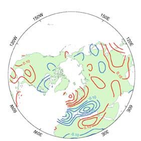
I. Fischer-Bruns et al.: Future impact of anthropogenic sulfate aerosol on North Atlantic climate

warming. This fact has been demonstrated by introducing              Planck Institute for Meteorology (MPI-M, Roeckner et al.
sulfate aerosol into climate models (e.g. Mitchell and Johns         1999). It consists of the atmospheric component ECHAM4,
1997; Reader and Boer 1998; Carnell and Senior 1998;                 a spectral transform model at T42 resolution employing 19
Roeckner et al. 1999). As SO2 emissions have harmful                 vertical levels, and the oceanic component OPYC3 (an
impacts on human health and natural environment, as they             updated version of the OPYC model developed by
cause for instance acid rain, many developed countries               Oberhuber 1993), which uses isopycnal coordinates at 11
have been reducing these emissions from power stations.              vertical levels. Both model components are coupled quasi-
Thus it can be anticipated that this compensating effect will        synchronously, exchanging daily averaged quantities once
be weaker in the future.                                             a day. The mixed layer temperature and the sea-ice vari-
   The effects of sulfate aerosol may be separated into the          ables are received by the atmospheric component without
‘direct effect’ in regions without clouds and ‘indirect              any adjustment. For the oceanic component solar radiation,
effects’ in cloudy regions. The direct aerosol effect on             river discharge, wind stress, and friction velocity are pas-
climate is due to scattering and absorption of sunlight. In          sed without adjustments as well. Restricted to heat and
case of scattering particles, the amount of sunlight that            freshwater only, non-seasonal constant flux adjustments
reaches the earth’s surface is reduced due to the presence of        were employed to prevent the model from drifting to an
the aerosol. Indirect effects are, for instance, the influence       unrealistic climate state. The adjustments were estimated
of the aerosol particles on cloud microphysical properties,          from a 100-year coupled model spin up. Details on the
such as reflectivity, lifetime and precipitation rates. An           coupling technique can be found in Bacher et al. (1998).
evaluation of the indirect effects and their consequences is            ECHAM4/OPYC3 is an AOGCM that has been used in
beyond the scope of this paper. In this study, we concen-            climate modeling studies by several research groups
trate on the possible future climatic changes in the North           worldwide. Work published earlier evaluated the perfor-
Atlantic region with special emphasis on the direct radia-           mance of the atmospheric model and the coupled model
tive impact of sulfate aerosol from anthropogenic origin.            (e.g. Roeckner et al. 1996a, b; Bacher et al. 1998; Roeckner
The direct aerosol forcing represents only a part of the             et al. 1999). Despite the restriction of the flux correction to
overall aerosol effect; therefore our work represents also           heat and freshwater only, the annual and seasonal climate
only a part of the entire picture of the aerosol’s role in our       of the coupled model agrees well with that produced by the
climate. We investigate a simulation forced by greenhouse            atmospheric model component alone, when it is forced
gases and a simulation forced by both greenhouse gases               with observed sea surface temperatures (SSTs). The cou-
and sulfate aerosol. Ulbrich and Christoph (1999) and                pled model captures many features of the observed
Knippertz et al. (2000) also analyzed the same simulation            interannual SST variability in the tropical Pacific, mainly
forced by greenhouse gases used in this study with respect           related to El Niño events. The results of the AOGCM show
to NAO and cyclone tracks. However, these studies do not             also adequate agreement with observations regarding the
take into account the additional effects of sulfate aerosol.         weakening of the westerlies across the North Atlantic in El
To our knowledge, such an isolation of the aerosol forcing           Niño/Southern Oscillation (ENSO) winters, as well as
effects on the climate change in a specific region has not           regarding the weak tendency for colder than normal win-
been attempted previously.                                           ters in Europe. Stephenson and Pavan (2003) compared the
   Details about the model and a description of the                  NAO simulated by the coupled model to observed data
experimental design are given in Sect. 2. In Sect. 3, we             together with the results of 16 other AOGCMs (see Sect.
describe the method to calculate the aerosol effect, our             4.5). Comparisons of modeled data with reanalysis data
significance test and the cyclone tracking method. Sec-              and observations that are made for this study will be shown
tion 4 presents the results for the direct aerosol effect upon       in Sects. 4.5–4.7.
temperature, radiative quantities, precipitation, NAO,
baroclinicity and cyclone track density. The paper is                2.2 Simulations
summarized and concluded in Sect. 5.
                                                                     We investigate two transient climate simulations
                                                                     (Roeckner et al. 1999). One of the simulations is forced
2 Model description and simulations                                  with time-dependent anthropogenic greenhouse gases alone
                                                                     (referred to as simulation GHG in the following). The
2.1 The climate model                                                second simulation additionally includes the backscattering
                                                                     of solar radiation due to the presence of sulfate aerosol
We analyze data of two transient model simulations per-              originating from anthropogenic sulfur emissions (GSD).
formed with the ECHAM4/OPYC3 coupled atmosphere–                     Natural biogenic and volcanic sulfur emissions are
ocean general circulation model (AOGCM) of the Max                   neglected. The GHG simulation has been performed for the

123
I. Fischer-Bruns et al.: Future impact of anthropogenic sulfate aerosol on North Atlantic climate
period (1860–2100), the GSD simulation for (1860–2050). 3 Methods
Since GSD is available only until 2050, we do not consider
the last 50 years of GHG. The simulations allow for a 3.1 Separating the aerosol effect
separation of the aerosol effect from the anthropogenic
greenhouse effect by building differences between the In order to separate the aerosol effect on different vari-
variables of both data sets (see Sect. 3.1). A third simula- ables, we calculate differences between the GSD and the
tion (GSDIO), which has also been published by Roeckner GHG simulation of 30-year averages of these variables.
et al. (1999), accounts for the influences of greenhouse Our analysis is restricted to a domain, which is limited to
gases, and additionally, ozone and considers both the direct the North Atlantic Ocean and surrounding land regions
and the indirect sulfate aerosol effects. The reason why the (90W–60E, 20–80N). Regions in this domain that show
GSDIO simulation is not evaluated here is that a separation significant differences are rather small for ‘present periods’
of the anthropogenic greenhouse gas effect and the aerosol like (1961–1990) and the influence of the aerosol turns out
effect would be impeded by the consideration of ozone. to be largest in a warmer climate. Thus we focus only on
In the simulations GHG and GSD, changes in con- the future climate and discuss mainly results for (2021–
centrations of the major greenhouse gases (CO2, CH4, 2050). Although photochemistry is more vivid in summer
N2O and certain halocarbons) are prescribed from 1860 to and hence the oxidation of sulfur dioxide yields a larger
1990 as observed. From 1991 to 2050 these concentra- amount of sulfate in summer than in winter, we only
tions are assumed as projected into the future according to consider boreal winter. The reason is that we are interested
the IPCC IS92a forcing scenario (Houghton et al. 1992). particularly in the NAO and the related North Atlantic
In simulation GSD the tropospheric sulfur cycle is fully storm tracks, and, in general, the winter exhibits most
coupled with the meteorology of the atmospheric com- intense extra-tropical storms. During the winter season, the
ponent ECHAM4 (Feichter et al. 1996, 1997). The sulfate NAO accounts for more than one-third of the total variance
mass mixing ratio computed by the model is transformed in sea level pressure (SLP) over the North Atlantic region
into particle number concentrations under the assumption (Hurrell et al. 2003). In the following, the year corresponds
of a log-normal size distribution. The wavelength to January for each winter season.
dependent optical properties are determined according to
Mie Theory. Transport and deposition processes are cal- 3.2 Significance testing
culated interactively. The simulated trend in sulfate
deposition in GSD since the end of the nineteenth century A widely used test for the comparison of two means is the
is broadly consistent with ice core measurements (Roe- Student’s t test. Apart from the distributional assumptions,
ckner et al. 1999). The assumed future emission of sulfur this test requires that the data samples are statistically
dioxide, also based on scenario IS92a, is higher than those independent. This assumption is mostly violated in clima-
for the six SRES emission scenarios (Nakicenovic and tological applications since the data are serially correlated
Swart 2000). The reason is that due to local air quality (Zwiers and von Storch 1995). In the following we do not
concerns in the industrialized countries, scenarios pub- address the problem of serial correlation. However, the
lished since 1995 assume sulfur controls of different Student’s t test should only be applied to data, which can be
degrees for the future. This fact had not been considered assumed as normally distributed and exhibiting comparable
at that time when the IS92a scenario was designed. The variances. In order to avoid these assumptions, we introduce
projected future increase in SO2 emissions by the devel- a non-parametric significance test. Taking the future tem-
oping countries is clearly visible in our simulations in a perature difference as an example, our null hypothesis is: the
shift in sulfate burden towards the equator, as will be difference (GSD–GHG) of the temperature averaged over
shown in Sect. 4.1. (2021–2050) lies within the range of the variations of dif-
The control simulation (CTL) is integrated over ferences of temperature averages over 30-year periods,
300 years and is driven with constant ‘present-day’ which are randomly chosen from the undisturbed CTL
greenhouse gas concentrations fixed at the observed 1990 simulation. This hypothesis is tested against the alternative
values (IPCC 1990). Industrial gases (like halocarbons and hypothesis that (GSD–GHG) exceeds this range: First we
others) are not considered. The prescribed concentrations determine m 30 year-averages from the CTL simulation
of aerosols and ozone are based on climatologies. There is (here m = 10) and subtract all these averages from each
no sulfur cycle in this simulation. The CTL simulation is other. The frequency distribution of the [m(m - 1)/2] = 45
used for comparisons with reanalysis data and for a non- differences is believed to represent an unbiased and robust
parametric significance test, which is described in Sect. 3.2. estimation of the true distribution. Finally, we have to
For more details on the model and the simulations we refer determine whether the difference (GSD–GHG) for (2021–
to Roeckner et al. (1999). 2050) is located ‘sufficiently far away’ in the tail of this
123I. Fischer-Bruns et al.: Future impact of anthropogenic sulfate aerosol on North Atlantic climate
distribution. If it is larger than e.g. the 95% percentile, we calculated in the GSD simulation according to the emis-
can be 95% certain that the difference is statistically sig- sions of sulfur dioxide projected in the IS92a scenario.
nificant. In other words, the null hypothesis can be rejected There is a strong increase in sulfate burden from ‘present-
with a risk of less than 5%. We have tested the significance day’ values (1961–1990) to the future period (2021–2050)
of all calculated differences (GSD–GHG) of variables (Fig. 1a, b). Due to the non-uniform distribution of sources,
averaged over (2021–2050) in this study with this method. the spatial distribution of the aerosol burden is also rather
The test has been performed at every grid point within our inhomogeneous. The source regions are clearly identified
model domain. The colored areas of Figs. 2, 3 and 10 show by the darker colored areas. The mean burden is highest in
regions with statistically significant differences at the 95% source regions and downstream of them. The difference in
level. Regions with no significant differences are masked burden between the averages over both periods (Fig. 1c)
out and white-colored. indicates a clear shift to the south. This shift is even more
obvious on the global scale (not shown). It is due to the
3.3 Cyclone tracking projected future decrease of SO2 emissions in the industrial
countries and the future increase in the developing
In this study, we use the feature tracking algorithm proposed countries.
by Hodges (1999). Before identifying the mean sea level
pressure (MSLP) minima in a data set with this method, it is 4.2 Temperature, surface albedo and short wave
recommended to remove wave numbers B5 from the MSLP radiation
field. The reason is that there is uncertainty whether a low
pressure system like the Icelandic low is formed by the The sulfate aerosol effect on the near surface winter tem-
successive movement of cyclones into the region or whether perature for (2021–2050) is displayed in Fig. 2a, showing
it is a feature of the planetary-scale background wave pat- the difference (GSD–GHG) between both simulations.
tern. The removal of the planetary-scale background Since the aerosol backscatters sunlight, this leads to a
accommodates both views (Hoskins and Hodges 2002). The cooling of the surface. Thus, the future temperature
algorithm tracks the MSLP minima in time by minimizing a increase due to the increase in anthropogenic greenhouse
cost function which poses constraints on the upper dis- gases is smaller in simulation GSD relative to GHG.
placement distance and the track smoothness to obtain the Averaged over the whole region, the ‘cooling’, which
minimal set of smoothest tracks. In order to be detected, a is actually an attenuation of the warming, amounts to
cyclone has to exist at least for 2 days and has to travel a -1.2K. There is no significant impact on temperature over
distance of at least 1,000 km. The track density is defined as the Labrador Sea and over Greenland, where the aerosol
the number of tracks passing through a unit area defined as a burden is lowest. Due to the slower decrease in sea ice and
circle of 5 radius (*106 km2) per winter. snow cover in the GSD simulation compared to GHG
(Roeckner et al. 1999), the decrease in the future mean
surface albedo is attenuated (Fig. 2b), which is indicated
4 Direct aerosol effect upon North Atlantic winter by positive values for (GSD–GHG). This happens over the
climate Arctic Ocean, where the albedo difference is largest (up to
30%), over some regions in northeastern Canada and
4.1 Sulfate aerosol burden northeastern Europe. As for temperature, no significant
impact on the mean surface albedo of Greenland is found.
Figure 1 shows a picture of the future growth and shift in Both the albedo effect and the aerosol backscattering effect
sulfate aerosol burden in extended boreal winter (DJFM) imply a smaller increase in net short wave (SW) clear-sky
(a) (b) (c)
Fig. 1 Geographic distribution of the calculated winter-mean (DJFM) anthropogenic sulfate aerosol burden in simulation GSD [mg SO4 m-2].
a Average over period (1961–1990), b average over period (2021–2050) and c difference between both multi-decadal averages
123I. Fischer-Bruns et al.: Future impact of anthropogenic sulfate aerosol on North Atlantic climate
(a) (b) (c)
Fig. 2 Difference (GSD–GHG) of averages over (2021–2050) net shortwave clear-sky radiation [Wm-2]. Areas where the differ-
between both simulations of the winter-mean (DJFM) a near surface ence is not statistically significant at the 95% level are masked white
temperature [K], b surface albedo [dimensionless units] and c TOA
radiation in the GSD simulation over most regions, again both simulations, we conclude that the aerosol impact on
with the exception of Greenland. This holds for the top-of- the greenhouse effect between both simulations is mainly
the-atmosphere (TOA, Fig. 2c) as well as for the surface due to the weakened increase in atmospheric temperature
(SFC, not shown). The patterns for TOA and SFC net SW and water vapor concentration. As the air in the GHG
radiation compare well with each other, since—unlike the simulation is warmer than in GSD, it can sustain higher
radiative impact of the greenhouse gases—the radiative concentrations of water vapor without becoming saturated.
forcing of the aerosol is changing the heat budget mainly at Consequently, more evaporation takes place and the con-
the earth’s surface and not that of the atmosphere (Roe- centration of water vapor may increase further. This in turn
ckner et al. 1999). Regions with the largest negative enhances the greenhouse effect and gives rise to further
differences (GSD–GHG) in TOA net SW radiation coin- warming. The aerosol impact on the greenhouse effect for
cide approximately with regions with the largest positive (2021–2050), shown in terms of LW radiation absorbed in
differences in surface albedo. the atmosphere, results in a weakening of this effect over
large regions (Fig. 3b). However, the highly non-linear
4.3 Long wave radiation surface emission effect is clearly larger than the water
vapor feedback (Roeckner et al. 1999), and the greenhouse
We also diagnose a weakened increase in the amount of effect is approximately proportional to the near surface
outgoing long wave radiation (OLR) emitted to space in the temperature. This becomes evident by a comparison of
GSD simulation compared to GHG for (2021–2050) Fig. 3b with the temperature difference pattern (Fig. 2a).
(Fig. 3a). This variable depends strongly on the SFC net
long wave (LW) radiation (not shown), which is balanced 4.4 Precipitation
by two radiative fluxes with opposite sign: the upward
infrared flux due to the LW earth’s surface emission and If we consider only the increasing anthropogenic green-
the downward infrared flux emitted by the atmosphere due house gases (as in GHG) we find a poleward displacement
to the greenhouse effect. According to Raval and Rama- of the mean winter precipitation pattern for (2021–2050)
nathan (1989) the latter is defined by the difference compared to the present (not shown). The associated pre-
between the OLR and the surface LW emission. Since the cipitation increase at higher latitudes is related to an
anthropogenic greenhouse gas concentrations are equal in increase in water vapor in the atmosphere arising from the
(a) (b) (c)
Fig. 3 As in Fig. 2, but for the difference in a clear-sky OLR [Wm-2], b LW radiation absorbed in the atmosphere [Wm-2] and c total
precipitation [mm day-1]
123I. Fischer-Bruns et al.: Future impact of anthropogenic sulfate aerosol on North Atlantic climate
warming of the oceans. The colder atmosphere in the GSD anomalies at every grid point in the model domain. The
simulation, however, has less capacity to hold moisture. NAO index is then represented by the PC time series
This reduces the mean water vapor column compared to corresponding to the leading EOF. Following this method,
GHG over the Northern parts of the North Atlantic Ocean Stephenson and Pavan (2003) validated the NAO in the
(not shown). The (GSD–GHG) precipitation patterns for CTL simulation investigated here together with 16 other
(2021–2050) show significant negative values in these AOGCMs in comparison to observations. They defined as
regions as well (Fig. 3c). Here the cooling effect is larg- NAO index the leading PC of the surface temperature
est. The negative values denote a significantly smaller anomalies, taking advantage of the more robust signature in
precipitation increase in a warmer climate when anthro- surface temperature to define this phenomenon. They
pogenic sulfate aerosol is considered additionally. demonstrated that ECHAM4-OPYC—as 12 other
AOGCMs—is able to capture the NAO pattern based on
4.5 North Atlantic Oscillation observations. However, they showed also that ECHAM4/
OPYC, as some other models, overestimates the observed
The North Atlantic Oscillation (NAO) is one of the most weak anti-correlation between the NAO temperature index
dominant modes of natural climate variability. It has strong and ENSO.
effects on weather and climate in the North Atlantic region. By applying the EOF technique to MSLP data, we
The term ‘NAO pattern’ has been given to the observed determine the NAO patterns from ECMWF reanalysis data
recurring pressure anomaly pattern due to a large-scale ERA-40 (for the years 1959–2001; Uppala et al. 2005) in
seesaw in atmospheric mass between the Azores high and comparison to the CTL simulation (1990 conditions) as
the Icelandic low. The NAO index describes the large-scale shown in Fig. 4a, d. The same technique is applied also to
atmospheric pressure difference between these regions and the GHG and GSD simulations for the periods (1861–1990)
is commonly used as an indicator for the strength of the and (2021–2050) (Fig. 4b, c, e, f). All panels in Fig. 4
westerlies over the eastern North Atlantic. In its positive show the same characteristic features of the typical NAO
phase it is associated with a deeper than normal Icelandic pattern: the two distinct centers of action located near
low and a stronger than normal Azores high. As a conse- Iceland and between the Azores and the Bay of Biscay. The
quence for Europe, enhanced westerlies bring more warm NAO pattern for CTL has a somewhat larger amplitude
moist air over the continent, resulting in warmer and wetter than ERA-40 near Iceland. Generally, the NAO in the CTL
than average winter conditions in northwestern Europe. simulation shows a greater influence over North Europe
Southern Europe tends then to be colder and drier. In its than is reflected by the reanalysis data. The ERA-40 pattern
negative phase weaker mean westerlies with corresponding explains the largest amount of total variance (52%), com-
colder and drier northwestern European winters occur, and pared with the modeled patterns. If we consider the panels
warm and wet conditions are dominating in the South. It is for the period (1861–1990) (Fig. 4b, c), it can be seen that
apparent that the NAO is controlling the position of the the GSD NAO pattern exhibits a greater extension to the
cyclone tracks and meteorological variables such as tem- East and suggests a different position of the jet stream than
perature, precipitation and surface wind speed. Over the the GHG pattern for this period. It matches better the ERA-
past years numerous scientific NAO-related articles have 40 pattern than GHG, since GHG shows a somewhat too
been published. For more information about this mode of weak amplitude of the Azores high. If we compare the
variability we refer to the basic publications (e.g. Hurrell GHG and GSD patterns projected into the future period
et al. 2003; Dickson et al. 2000) and the references cited (2021–2050) (Fig. 4e, f), it becomes apparent that in GHG
therein. There is public concern if there will be a change in this amplitude is even more weakened (Fig. 4e), whereas
the occurrence of cyclones with global warming associated the subtropical high pressure region is most pronounced
with extreme NAO or heavy storm events. In this study we and elongated for the GSD simulation in the future period
are interested in whether the direct aerosol effect has the (Fig. 4f).
potential to influence the structure and temporal evolution The associated PC time series, which represent the NAO
of the NAO and the mean position and density of the indices, are shown in Fig. 5 for ERA-40 (1959–2001), the
cyclone tracks. CTL simulation (300 years), and the GHG as well as GSD
The temporal evolution of the NAO pattern can be simulation for the entire period (1861–2050). Each NAO
characterized by different kinds of NAO indices. One time series is standardized by subtraction of its mean and
method to determine NAO pattern and index is the widely division by its standard deviation r. The modeled NAO
used empirical orthogonal function (EOF) analysis—or indices generally show a strong year-to-year variability.
principal component (PC)—technique. Here the NAO The known upward trend in the observed NAO index can
pattern is identified from the eigenvectors of the cross- be seen in the ERA-40 data. Since 1980, the NAO has
correlation matrix, computed e.g. from the MSLP remained mostly in a positive phase. If we consider the
123I. Fischer-Bruns et al.: Future impact of anthropogenic sulfate aerosol on North Atlantic climate
(a) (b) (c)
(d) (e) (f)
Fig. 4 Leading EOFs of North Atlantic sea level pressure anomalies (2021–2050), f GSD simulation (2021–2050). Contour interval is
based on winter (DJFM) means of a ERA-40 (1959–2001) reanalysis, 0.5 [hPa], positive values are shaded. The percentage of the total
b GHG simulation (1861–1990), c GSD simulation (1861–1990), d variance accounted by these modes is indicated in the headlines
CTL simulation (1990 conditions, 300 years), e GHG simulation
(a) (b) (c) (d)
Fig. 5 NAO indices associated to the patterns in Fig. 4 for a ERA-40 dimensionless time series are standardized to have unit variance. The
(1959–2001) reanalysis, b CTL simulation (300 years), c GHG horizontal lines indicate ±1r
simulation (1861–2050), and d GSD simulation (1861–2050). The
simulations over the whole period (1861–2050), no sig- NAO- is well balanced (16 NAO?, 17 NAO-). CTL
nificant linear trend can be identified in either NAO index exhibits more NAO?events, but less NAO- events than in
for GHG and GSD. This can be seen easily already by GHG for (1861–1990) (14 NAO?, 21 NAO-), respectively
visual inspection. The trend lines are nearly in accordance than in GSD for (1861–1990) (12 NAO?, 19 NAO-).
with the zero lines (not shown). Also the non-linear trends, Projecting into the future period (2021–2050), the number
obtained according to Ulbrich and Christoph (1999) from of NAO? increases strongly in GHG, whereas the number
quadratic curve fitting, are not significant in that sense that for NAO- decreases (23 NAO?, 10 NAO-). By addi-
they do not exceed the level defined by 1r, at least until tionally considering the counteracting cooling of the sulfate
year 2050. Comparing the unstandardized time series (not aerosol, this strong increase, respectively decrease, is
shown) with each other, we find that both variabilities are dampened (20 NAO?, 17 NAO-), working towards a
quite similar (rGHG = 1.70, rGSD = 1.74). However, both balance between both cases as we have found in the
simulations differ concerning the number of extreme NAO undisturbed CTL simulation.
events, which we define as winters with NAO indices
above (NAO?) and below 1r (NAO-). The numbers of 4.6 NAO correlation patterns
‘extreme’ NAO events occurring per century are shown in
Fig. 6 for the different simulations and periods. In the In the previous section we have defined the NAO in terms
undisturbed CTL simulation, the occurrence of NAO?and of pressure. However, as mentioned before, the NAO is
123I. Fischer-Bruns et al.: Future impact of anthropogenic sulfate aerosol on North Atlantic climate
temperature, respectively local precipitation. The patterns
show the northern hemispheric ‘spatial signature’ of the
NAO. Generally, in the case of a positive NAO index,
positive correlations indicate that the area is wetter or
warmer than normal; negative correlations represent an
area drier or colder than normal. Conditions are reversed in
the case of a negative NAO index. No correlation means
the area is unaffected by the NAO. In positive NAO pha-
ses, more and strong winter storms are crossing the Atlantic
Ocean on a track shifted to the north. Hence, mean warm
and wet winter climate in central and northern Europe is
observed, whereas cold and dry climate conditions prevail
in the Mediterranean, northern Africa and over the Arabian
Peninsula. On the other hand, a positive NAO index is also
associated with more frequent, cold dry air outbreaks from
Labrador. Thus, the climate is cold and dry over northern
Canada and Greenland, but warm and wet for the eastern
Fig. 6 Number of extreme NAO events per century for the different American continent. (Figs. 7a, 8a) For low NAO phases,
simulations and different time periods. NAO? (NAO-) denotes NAO
index above (below) 1r
these climate conditions are reversed. It is obvious that
especially the NAO-temperature correlation pattern is
dominated by a large-scale quadrupole pattern with centers
also strongly related to the mid-latitude variations in the over Northwest Europe and the northwest Atlantic char-
seasonal means of different meteorological variables such acterizing the northern seesaw. The centers over the United
as near surface temperature, SLP, and hydrological quan- States and the Middle East are reflecting the southern
tities. It accounts for much of their variability on seesaw. The relationship between NAO and temperature is
interannual and longer time scales over the Euro–Atlantic strongest over Southern Scandinavia and Finland. The
region. This leads us to investigate the correlation between correlations based on the model simulations (Figs. 7 and
the pressure based NAO index and the near surface tem- 8b–f, respectively) are computed at each grid point of the
perature, as well as between NAO and precipitation, for the Northern Hemisphere (20–80N). The model results are
different time periods. We are interested in how the mod- statistically significant at the 95% level according to a
eled correlation patterns look like in the present climate Student’s t test. Areas with no significant correlations are
and in a warmer climate with and without the influence of masked out after having computed the isolines.
the sulfate aerosol. For an evaluation of the model’s skill in At first we analyze the spatial signature of the NAO
generating the present correlation patterns, we first com- with respect to temperature in Fig. 7. In accordance with
pare model results with correlation maps based on Stephenson and Pavan (2003) both seesaws are described
observed datasets (from Osborn et al. 1999). Here the quite realistic by the CTL simulation (Fig. 7d). The
observational temperature data, a composition of SST observed seesaws are captured as well in the simulations
anomalies and 1.5 m air temperature anomalies over land, GHG and GSD (Fig. 7b, c) for data covering the time
were derived from instrumental measurements on a period (1861–1990). No striking difference concerning the
53 9 53 grid box basis. They cover the period 1873–1995. structure between the CTL and GHG nor the GSD pattern
The observational precipitation data set, also on a 53 9 53 is found. There are, however, differences in magnitude. For
grid box basis, contains data from 1900 to 1995 for land the GSD simulation (1861–1990) we get higher positive
areas only, derived from rain-gauge measurements. For the correlations compared to GHG (1861–1990) especially
determination of the observed NAO index (DJFM) Osborn over eastern North America and Russia. Thus they are in
et al. (1999) used two time series of station pressure. The better accordance with the magnitudes in the CTL pattern
index had been calculated by the absolute pressure differ- than GHG. The corresponding patterns in a warmer climate
ence between Gibraltar and southwest Iceland. For more (Fig. 7e, f) illustrate that the relationship NAO-temperature
details we refer to their above-mentioned publication. varies significantly depending on the time period. The
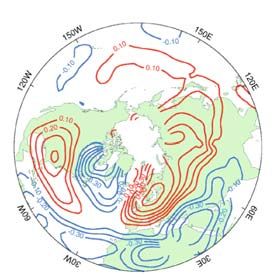
Figures 7 and 8 show the spatial correlation patterns comparison of Fig. 7b with and Fig. 7e shows that with
based on observations and the simulations for the different increase of anthropogenic greenhouse gas concentrations
time periods. Figures 7a and 8a (which are adopted from correlations increase slightly in the main centers of NAO
Osborn et al. 1999) show correlations as observed between influence over the North Atlantic Ocean, Europe and North
the normalized NAO index and local near surface Africa. On the other hand, large areas of significant NAO-
123I. Fischer-Bruns et al.: Future impact of anthropogenic sulfate aerosol on North Atlantic climate
(a) (b) (c)
(d) (e) (f)
Fig. 7 Correlation map of winter (DJFM) mean near surface simulation (2021–2050). Positive isolines are depicted in red,
temperature with the normalised NAO SLP index. a As observed negative isolines in blue. Isoline values are ±(0.1, 0.2, 0.3,…, 1).
(1873–1995, from Osborn et al. 1999), b in GHG simulation (1861– In b–f areas where the difference is not statistically significant at the
1990), c in GSD simulation (1861–1990), d in CTL simulation (1990 95% level are masked white
conditions, 300 years), e in GHG simulation (2021–2050), f in GSD
temperature correlation as observed in the current climate for the future period with those for (1861–1990) for both
have disappeared (over eastern America and the central GHG and GSD also reveals (as in case for temperature)
North Atlantic as part of the southern seesaw, and over that the additional consideration of sulfate induces a ten-
parts of the Middle East as well, Fig. 7e). For GSD (2021– dency to higher correlations, respectively anti-correlations,
2050), however, the NAO influence over Eastern North over large areas in the future period, especially over the
America remains, although there is a reduction in extent central North Atlantic Ocean.
and strength compared with GSD (1861–1990) (Fig. 7c, f).
Generally, the centers of NAO influence show a larger 4.7 Baroclinicity and cyclone tracks
extent and strength for GSD (2021–2050), where the future
warming is attenuated due to the influence of the sulfate Extratropical synoptic weather systems determine the local
aerosol, compared with GHG (2021–2050), where future day-to-day weather and play an important role in regulating
warming is larger due to the lack of the aerosol. This is in the transport of water, heat and momentum. Thus, we
accordance with the difference in spatial structure of the would like to know if the aerosol has an impact on the
southern center in the corresponding NAO patterns shown North Atlantic cyclone tracks. A primary mechanism for
in Fig. 5e, f for GHG (2021–2050) and GSD (2021–2050). the development of extratropical cyclones is the baroclinic
The comparison of the modeled NAO-precipitation instability, the atmospheric potential for forming cyclones.
correlation patterns with observations is restricted, since The baroclinicity during the first stages of the cyclogenesis
the latter cover land areas only. The observations show that can be quantified in terms of the maximum linear growth
north of 50N positive NAO values are associated with a rate rBI of the baroclinic instability (Eady 1949). The so-
precipitation increase, whereas over the Mediterranean called Eady growth rate is defined by the ratio of thermal
region correlations are negative. This is reflected also in the wind to static stability: rBI = 0.31(f/N)|qu/qz|. Here, f is
modeled patterns for GHG (1861–1990), GSD (1861– the Coriolis parameter, qu/qz the vertical wind shear and N
1990) and CTL (Fig. 8b–d). A comparison of the patterns the Brunt–Väisälä frequency (Lindzen and Farrell 1980;
123I. Fischer-Bruns et al.: Future impact of anthropogenic sulfate aerosol on North Atlantic climate
(a) (b) (c)
(d) (e) (f)
Fig. 8 Correlation maps of winter (DJFM) precipitation with the normalised NAO SLP index. a As observed (1900–1995, but land-only, from
Osborn et al. 1999), b–f as in Fig. 7 but for precipitation
Hoskins and Valdes 1990). The Eady growth rate is often The lower panels in Fig. 9 display the track density
referred to as the simplest measure for the baroclinicity of determined by the method described in Sect. 3.3. As for
the basic flow in the literature. We use the lower tropo- baroclinicity, the result for GHG (1961–1990) differs only
spheric maximum Eady growth rate at 775 hPa (i.e. for the slightly from CTL and thus we show only results for the
layer 700–850 hPa) as a measure for the atmosphere’s reanalysis and CTL, which we compare with the upper
potential to produce cyclones. A high growth rate favours a panels in Fig. 9. The North Atlantic Ocean is a region where
frequent development of cyclones and indicates the region new storms intensify or older storms redevelop. Since the
where the jet stream is located. cyclones propagate as they develop, they reach maturity
To evaluate the performance of the model we first further downstream along the cyclone track. Accordingly,
compare the baroclinicity as calculated from the reanalysis regions of maximum track density are not coincident with
data with the baroclinicity as simulated for 1990 condi- regions of maximum baroclinicity. The baroclinicity is
tions. Figure 9a shows the climatological maximum Eady largest at the beginning of the North Atlantic storm track, off
growth rate (referred to henceforth as simply ‘baroclinici- the East coast of North America, where the atmosphere is
ty’) for winter from ERA-40 reanalysis data averaged over most unstable due to the strong diabatic heating. The regions
(1961–1990). Regions of enhanced baroclinicity, i.e. with largest track density as found in ERA-40 (Fig. 9c) are
regions of cyclogenesis, can be found south of Nova Scotia depicted in comparison to the enhanced cyclonic activity in
extending northeastward to western Europe. Increased CTL (Fig. 9d). The reanalysis shows a band expanding from
baroclinicity is also apparent over North Africa and the the east coast of North America via Greenland and Iceland
Arabian Peninsula. The regions of high baroclinicity are into the Norwegian Sea and Barents Sea, as well as a less
generally in good agreement with the results for the CTL pronounced local maximum in the Mediterranean. The
simulation (Fig. 9b), especially over the East coast of comparison reveals fewer cyclones in the CTL simulation as
North America and the Atlantic Ocean. Some discrepancies observed in the region of the Great Lakes, near the Denmark
can be found over Greenland, the Barents Sea as well as Strait, to the west and north of Scandinavia and in the
North Africa. The correspondent figure for GHG (1961– Mediterranean. Maximum track densities occur near Nova
1990) is not shown since it agrees very well with CTL. Scotia and Newfoundland, in the Davis Strait and in the
123I. Fischer-Bruns et al.: Future impact of anthropogenic sulfate aerosol on North Atlantic climate
Fig. 9 Upper panels 850– (a) (b)
700 hPa maximum Eady growth
rate (DJF) [day-1] a from ERA-
40 reanalysis data averaged over
1961–1990, and b for the CTL
simulation. Lower panels c and
d as upper panels but for track
density [number densities per
month per 106 km2]. Track
density suppression threshold is
0.2
(c) (d)
Denmark Strait. On the other hand, more cyclones than in increase to the east of Greenland and north of 65N. The
ERA-40 occur around the Caspian Sea and especially over distinct regions with significant negative and positive dif-
the European part of Russia and near the Black Sea. How- ferences give the overall picture of a poleward transition of
ever, the overall agreement between CTL and ERA-40, the cyclone tracks. However, we obtain large regions in
especially over the North Atlantic Ocean and Western Fig. 10a with insignificant changes, masked in white,
Europe, gives confidence in the performance of the model instead of a significant increase in baroclinicity related to
and the tracking algorithm (Banse 2008). the regions of increased track density with future warming
Figure 10a, c shows the projected future change in over the northern North Atlantic, as could be expected.
baroclinicity and track density without consideration of the To find out if the direct aerosol effect has an impact on
cooling sulfate aerosol. The panels depict the differences in the simulated cyclone tracks in (2021–2050), we calculate
both quantities between (2021–2050) and (1961–1990) in the difference (GSD–GHG) for baroclinicity and track
the GHG simulation. Areas of decreased baroclinicity density over this period (Fig. 10b and d). Positive differ-
dominate the pattern in Fig. 10a, concentrating in one band ences in Fig. 10b denote a smaller future decrease in
from the East coast of North America over the Atlantic baroclinicity in GSD compared to GHG. Regions with
Ocean to Southern Europe/North Africa and further to the significant differences are found over the Labrador Sea
Northeast to the Caspian Sea. Decreased atmospheric along the East coast of Greenland, north of 65N, reaching
potential to form cyclones can also be found over the Finland and Russia. Large differences can be seen also over
Labrador Sea and Greenland Sea and further to the East. the Gulf of Mexico extending to the East and over West-
The decrease in baroclinicity can be associated with a Africa. The sulfate effect on change in track density is
decrease in the meridional SST gradient under enhanced shown in Fig. 10d. Here, negative values denote a smaller
greenhouse gas concentrations (not shown), since the high future increase and positive values a smaller future decrease
latitudes warm more than the lower ones. This can be in track density. Though, after application of the signifi-
related to the reduction in track density in Fig. 10c for GHG cance test, a smaller increase in track density is found only
in a region extending from the British Isles over the over some isolated regions over the northern North Atlantic
Southeast of Europe to eastern Russia—regions located Ocean (Fig. 10d). Areas with significant smaller decreases
downstream of the regions with largest decreases in baro- (positive values) are only found over Baffin Island and over
clinicity. A significant decrease in track density is also a small region in Russia. Larger areas with significant
apparent along the American coast north of 35N and over changes, as we expected to find over Europe or adjacent
Baffin Island. On the other hand, there is a strong significant regions in the South, however, cannot be diagnosed.
123I. Fischer-Bruns et al.: Future impact of anthropogenic sulfate aerosol on North Atlantic climate
Fig. 10 Upper panels (a) (b)
Difference in 850–700 hPa
maximum Eady growth rate
(DJF) [10-3 day-1] between a
(2021–2050) and (1961–1990)
in simulation GHG, and b
difference (GSD–GHG)
between both simulations over
period (2021–2050). Lower
panels c and d as upper panels
but for track density [number
densities per month per
106 km2]. Track density
suppression threshold is 0.2.
Areas where the difference is
(c) (d)
not statistically significant at the
95% level are masked white in
all panels
5 Summary and conclusions They focus on the period (2030–2050), where the pro-
jected aerosol forcing was maximum, with sulfur dioxide
We know that even though aerosols represent but a emissions based on the same scenario as here. However,
marginal fraction of the atmospheric mass, they play an the authors make a simplified approach in representing the
important role in our climate, because they interfere with backscattering of solar radiation by merely increasing the
the radiative transfer through the atmosphere. This surface albedo. Consistent to our results, they find a
implies that the influence of aerosols should not be pronounced cooling in boreal winter over the northern
neglected in climate studies. In this model study we midlatitude continents due to sulfate aerosol. It is obvious
investigate the possible future climate changes due to the that the main effect of scattering aerosols is a reduction of
impact of the direct clear-sky radiative forcing associated the anthropogenic warming due to the significant changes
with anthropogenic sulfate aerosol using ECHAM4/ in radiation, although the influence of the long-lived
OPYC3. We concentrate on the North Atlantic region and greenhouse gases on the mean temperature overwhelms
the winter season. Two different transient climate simu- the partially compensating influence of the short-lived
lations including the anthropogenic greenhouse effect are aerosols. We suppose that the differences in temperature
examined. One simulation considers additionally future and precipitation (as shown in Fig. 2a and 3c) are due
concentrations of sulfate aerosol. We are linking results initially to the radiation changes and as a consequence,
concerning temperature, radiative quantities, precipitation, the NAO pattern may change. The poleward extension of
and the NAO with the response in baroclinicity and the aerosol induced cooling is caused by the difference in
cyclone track density. In order to evaluate whether our snow and sea-ice cover and associated feedbacks in the
results are statistically significant, we introduce a non- higher latitudes. If aerosols are neglected, as in simulation
parametric significance test. In doing so, we can avoid the GHG, we find that the magnitude of the anthropogenic
assumptions of normality and comparable variances as warming is overestimated. As a consequence a poleward
required in a Student’s t test. Our test is recommended for shift of the patterns of NAO related quantities emerge,
comparisons of model data when a long control run is and a shift in NAO intensity towards a high index. For
available. Generally, we get a similar but weaker future the investigations of the NAO, we use pressure based
climate response due to the presence of the sulfate. This EOF analyses. Ulbrich and Christoph (1999) who also
attenuation is consistent with the findings of Mitchell and investigated the CTL and the GHG simulation, found a
Johns (1997), who compared the global response patterns northeastward shift of the NAO centers with enhanced
of two AOGCM simulations as well, one forced by greenhouse gas concentrations in the GHG simulation.
greenhouse gas alone, and one including sulfate aerosol. Though, their NAO index is determined by computing the
123I. Fischer-Bruns et al.: Future impact of anthropogenic sulfate aerosol on North Atlantic climate
difference between area averaged MSLP anomalies and Ocean and Western Europe. Concerning the poleward
has been related to the standard deviation of the CTL shift of the cyclone tracks in the simulation without
simulation. Moreover, their model domain is chosen consideration of aerosols, our results agree with many
somewhat different (90W–30E, 20–90N) compared to other studies (e.g. Schubert et al. 1998; König et al. 1993;
this study. In accordance to their results, our analysis Yin 2005; Bengtsson et al. 2006). There are indications
reveals a future change of the spatial characteristics of the that this shift is attenuated if sulfate is considered addi-
NAO in GHG, namely a shift of the NAO pattern to the tionally, since due to the cooling of the aerosol, there is a
East accompanied by an increase of extreme NAO? and a smaller decrease in baroclinity in the future climate than
decrease of extreme NAO- events compared to the period in GHG. We expected this to be related to a smaller
(1861–1990). Further we demonstrate that if sulfate is increase in track density north of 50N. However, a sig-
considered additionally, the tendency to an imbalance in nificant aerosol impact on the track density can be found
extreme NAO cases is reversed, although we see no only over some relatively small, isolated regions over the
indication of any dramatic changes like significant future northern North Atlantic Ocean. The fact that there is no
trends in the NAO index in either simulation, if we clear signal implies that the natural variability of the
consider the whole simulation (1861–2050). However, if related variables in this region is large.
e.g. only the period (2001–2050) is considered, which As the performance of a numerical climate model is
includes the strong trend in emissions of anthropogenic always limited, one caveat of this study—and of many
greenhouse gases, a positive trend in GHG, but a negative other climate studies—is that the results are obtained only
trend in GSD becomes apparent (not shown). This is in by one single model and one realization of each simula-
accordance with the occurrence of more NAO? than tion. Moreover, there is some evidence that mechanisms
NAO- extremes in the period GHG (2021–2050), which involving the stratosphere can influence the NAO, though
also represents an indication for an upward trend. The the extent of this interaction is still an open question (e.g.
correlation patterns of NAO with temperature and pre- Vallis and Gerber 2008, and references cited therein).
cipitation, respectively, for both GHG and GSD, are in Furthermore, the direct aerosol forcing represents only
good agreement with the observations for the time period one part of the overall aerosol effect. Here we disregard
up to the present. The outstanding characteristics of the indirect aerosol effects as well as the effects of some
NAO-temperature quadrupole pattern are captured in all major aerosol components such as absorbing carbona-
simulations. A particular interesting feature is the overall ceous aerosols. Still, we consider the present study to be
robustness of this pattern, which does not depend cru- relevant for understanding the North Atlantic climate with
cially on the type of the forcing in our simulations—at increasing anthropogenic warming and simultaneous
least up to the present. The future strong greenhouse gas consideration of scattering aerosol. Our results emphasize
forcing in GHG, though, tends to reduce the extent of the the view that changes in the atmospheric aerosol load
regions, where the NAO has an influence. This applies in have the potential to influence large-scale circulation over
particular to correlations between NAO and temperature. the North Atlantic. Clearly, this study cannot provide
Especially, we find no more influence of the NAO over information on climate effects due to the full suite of
the southeastern United States, in such a way that positive aerosol components and related processes, which are a
NAO events are associated with warmer and wetter subject of our ongoing research. The consideration of
winters. But if the strong future anthropogenic warming is indirect aerosol effects is also required in future simula-
dampened by the cooling effect of the aerosol, the regions tions, in particular to address issues associated with
of NAO influence—particularly for temperature—exhibit aerosol-cloud interactions.
again a larger areal extent with stronger correlations
(Fig. 7f compared to Fig. 7e). This is in accordance with Acknowledgments This work was funded by the ‘Sonderfors-
chungsbereich’ (SFB) 512 sponsored by the ‘Deutsche
the difference in spatial structure in the corresponding Forschungsgemeinschaft’ (DFG). We thank E. Roeckner for helpful
NAO patterns (Fig. 4e, f). Our results lead us to conclude suggestions. Discussions with S. Kinne and M. Giorgetta were con-
that future NAO changes become more important for the structive and helpful as well. Furthermore we would like to thank
North Atlantic winter climate when the direct aerosol K. Hodges for providing the tracking method and are grateful to
T. Osborn for supplying the figures of the correlation patterns based
effect in our model is considered additionally, since we on observations. We also appreciate the help of Norbert Noreiks and
find larger regions of influence and a tendency to higher Elisabeth Viktor in adapting the figures.
correlations, respectively anti-correlations.
The model is also capable in reproducing the main Open Access This article is distributed under the terms of the
Creative Commons Attribution Noncommercial License which
features of the storm track. The simulated cyclone track permits any noncommercial use, distribution, and reproduction in
density for ‘present day’ climate is in satisfying agree- any medium, provided the original author(s) and source are credited.
ment with the ERA-40, at least over the North Atlantic
123I. Fischer-Bruns et al.: Future impact of anthropogenic sulfate aerosol on North Atlantic climate
References König W, Sausen R, Sielmann F (1993) Objective identification of
cyclones in GCM simulations. J Clim 6:2217–2231. doi
Bacher A, Oberhuber JM, Roeckner E (1998) ENSO dynamics and :10.1175/1520-0442(1993)006\2217:OIOCIG[2.0.CO;2
seasonal cycle in the tropical Pacific as simulated by the Lindzen RS, Farrell B (1980) A simple approximate result for the
ECHAM4/OPYC3 coupled general circulation model. Clim Dyn maximum growth rate of baroclinic instabilities. J Atmos
14:431–450. doi:10.1007/s003820050232 Sci 37:1648–1654. doi :10.1175/1520-0469(1980)037\1648:
Banse DF (2008) The influence of aerosols on North Atlantic ASARFT[2.0.CO;2
cyclones. PhD thesis, University of Hamburg. Reports on Earth Mitchell JFB, Johns TC (1997) On modification of global warming by
System Science 53, ISSN 1614–1199, Max-Planck-Institute for sulfate aerosols. J Clim 10:245–267. doi :10.1175/1520-0442
Meteorology, Hamburg, Germany (1997)010\0245:OMOGWB[2.0.CO;2
Bengtsson L, Hodges KI, Roeckner E (2006) Storm tracks and climate Nakicenovic N, Swart R (eds) (2000) Special Report on Emissions
change. J Clim 19:3518–3543. doi:10.1175/JCLI3815.1 Scenarios, Cambridge University Press, Cambridge, UK
Bellouin N, Boucher O, Haywood J, Reddy MS (2005) Global Oberhuber JM (1993) Simulation of the Atlantic circulation with a
estimate of aerosol direct radiative forcing from satellite coupled sea ice mixed layer-isopycnal general circulation model.
measurements. Nature 438:1138–1141. doi:10.1038/nature Part I: model description. J Phys Oceanogr 23:808–829. doi
04348 :10.1175/1520-0485(1993)023\0808:SOTACW[2.0.CO;2
Carnell RE, Senior CA (1998) Changes in midlatitude variability due Osborn TJ, Briffa KR, Tett SFB, Jones PD, Trigo RM (1999)
to increasing greenhouse gases and sulfate aerosols. Clim Dyn Evaluation of the North Atlantic Oscillation as simulated by a
14:369–383. doi:10.1007/s003820050229 coupled climate model. Clim Dyn 15:685–702. doi:10.1007/
Dickson RR, Osborn TJ, Hurrell JW, Meincke J, Blindheim J, s003820050310
Adlandsvik B et al (2000) The Arctic Ocean response to the Raval A, Ramanathan V (1989) Observational determination of the
North Atlantic Oscillation. J Clim 13:2671–2696. doi :10.1175/ greenhouse effect. Nature 342:758–762. doi:10.1038/342758a0
1520-0442(2000)013\2671:TAORTT[2.0.CO;2 Reader MC, Boer GJ (1998) The modification of greenhouse gas
Eady ET (1949) Long waves and cyclone waves. Tellus 1:33–52 warming by the direct effect of sulfate aerosols. Clim Dyn
Feichter J, Kjellström E, Rohde H, Dentener F, Lelieveld J, Roelofs 14:593–607. doi:10.1007/s003820050243
GJ (1996) Simulation of the tropospheric sulfur cycle in a global Roeckner E, Arpe K, Bengtsson L, Christoph M, Claussen M,
climate model. Atmos Environ 30:1693–1707. doi:10.1016/ Duemenil L et al (1996a) The atmospheric general circulation
1352-2310(95)00394-0 model ECHAM-4: model description and simulation of present-
Feichter J, Lohmann U, Schult I (1997) The atmospheric sulfur cycle day climate. MPI Report No. 218, Max-Planck-Institute for
and its impact on the short wave radiation. Clim Dyn 13:235– Meteorology, Hamburg
246. doi:10.1007/s003820050163 Roeckner E, Oberhuber JM, Bacher A, Christoph M, Kirchner I
Forster PM et al (2007) Changes in atmospheric constituents and in (1996b) ENSO variability and atmospheric response in a global
radiatve forcing. In: Solomon S, Qin D, Manning M, Chen Z, coupled atmosphere–ocean GCM. Clim Dyn 12:737–754. doi:
Marquis M, Averyt KB, Tignor M, Miller HL (eds) Climate 10.1007/s003820050140
change 2007: the physical science basis. Contribution of working Roeckner E, Bengtsson L, Feichter J, Lelieveld J, Rodhe H (1999)
group I to the fourth assessment report of the intergovernmental Transient climate change simulations with a coupled atmo-
panel on climate change. Cambridge University Press, Cambridge sphere–ocean GCM including the tropospheric sulfur cycle. J
Hodges KI (1999) Adaptive constraints for feature tracking. Mon Clim 12:3004–3032. doi :10.1175/1520-0442(1999)012\3004:
Weather Rev 127:1362–1373. doi :10.1175/1520-0493(1999) TCCSWA[2.0.CO;2
127\1362:ACFFT[2.0.CO;2 Schubert M, Perlwitz Ja, Blender R, Fraedrich K, Lunkeit F (1998)
Hoskins BJ, Valdes PJ (1990) On the existence of storm-tracks. J North Atlantic cyclones in CO2-induced warm climate simula-
Atmos Sci 47:1854–1864. doi :10.1175/1520-0469(1990)047\ tions: frequency, intensity, and tracks. Clim Dyn 14:827–837.
1854:OTEOST[2.0.CO;2 doi:10.1007/s003820050258
Hoskins BJ, Hodges KI (2002) New perspectives on the northern Stephenson DB, Pavan V (2003) The North Atlantic Oscillation in
hemisphere winter storm tracks. J Atmos Sci 59:1041–1061. doi coupled climate models: CMIP1 evaluation. Clim Dyn 20:381–
:10.1175/1520-0469(2002)059\1041:NPOTNH[2.0.CO;2 399
Houghton JT, Callander BA, Varney SK (eds) (1992) Climate change Ulbrich U, Christoph M (1999) A shift of the NAO and increasing
1992: the supplementary report to the IPCC scientific assess- storm track activity over Europe due to anthropogenic green-
ment. Cambridge University Press, Cambridge house gas forcing. Clim Dyn 15:551–559. doi:10.1007/
Hurrell JW, Kushnir Y, Ottersen G, Visbeck M (2003) An overview s003820050299
of the North Atlantic Oscillation. In: Hurrell JW, Kushnir Y, Uppala SM et al (2005) The ERA-40 re-analysis. Quart J Roy Meteor
Ottersen G, Visbeck M (eds) The North Atlantic Oscillation: Soc 131B:2961–3012
Climatic significance and environmental impact. Geophysical Vallis GK, Gerber EP (2008) Local and hemispheric dynamics of the
Monographs Series, vol 134. pp 1–35 North Atlantic Oscillation, annular patterns and the zonal index.
IPCC (1990) Intergovernmental panel on climate change. In: Dyn Atmos Oceans 44:184–212. doi:10.1016/j.dynatmoce.
Houghton JT, Jenkins GJ, Ephraums JJ (eds) Scientific assess- 2007.04.003
ment of climate change. Cambridge University Press, Yin JH (2005) A consistent poleward shift of the storm tracks in
Cambridge, 365 pp simulations of 21st century climate. Geophys Res Lett
Knippertz P, Ulbrich U, Speth P (2000) Changing cyclones and 32:L18701. doi:10.1029/2005GL023684
surface wind speeds over the North Atlantic and Europe in a Zwiers FW, von Storch H (1995) Taking serial correlation into
transient GHG experiment. Clim Res 15:109–122. doi:10.3354/ account in tests of the mean. J Clim 8:336–351. doi :10.1175/
cr015109 1520-0442(1995)008\0336:TSCIAI[2.0.CO;2
123You can also read