Design of an attitude control algorithm based on data from a single horizon sensor
←
→
Page content transcription
If your browser does not render page correctly, please read the page content below
University Degree in Aerospace Engineering
                      Academic Year 2018-2019

                            Bachelor Thesis

 “Design of an attitude control algorithm
  based on data from a single horizon
                 sensor”

                        Alberto Jódar Moya

                     Javier Rodríguez Rodríguez
                          Leganés, June 2019

[Include this code in case you want your Bachelor Thesis published in Open Access
University Repository]
This work is licensed under Creative Commons Attribution – Non Commercial –
Non Derivatives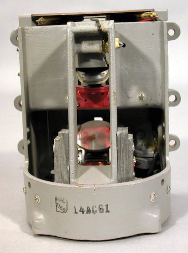
SUMMARY

Keywords: satellite, space, orbit, smallsat, CubeSat, gravity gradient, torque, angular
velocity, Euler angles, algorithm, Mean Square Error

                                                                                    iii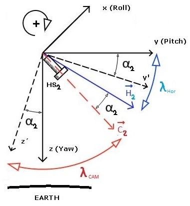
DEDICATION

First of all, I want to thank my professor Javier Rodríguez, for being an extraordinary
guide for the project. Thank you for introducing this project to me, it has been a lot of
fun.
To the guys, because my university experience would not have been the same.
To my family, thank you. Thank you for being always and always and always there. I’m
sure I would not have been able to make it without your support. Thanks for believing in
a different lifestyle. Thank you for believing in me.

                                                                                       v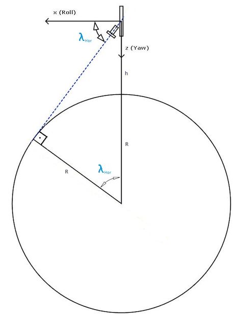
CONTENTS

1. INTRODUCTION. . . . . . . . . . . . . . . . . . . . . . . . . . . . . . . . . . . .             1
 1.1. State of the art . . . . . . . . . . . . . . . . . . . . . . . . . . . . . . . . . . . .     2
 1.2. Socio-economic impact . . . . . . . . . . . . . . . . . . . . . . . . . . . . . . .          2
 1.3. Motivation . . . . . . . . . . . . . . . . . . . . . . . . . . . . . . . . . . . . . .       3
 1.4. Objectives. . . . . . . . . . . . . . . . . . . . . . . . . . . . . . . . . . . . . . .      3
 1.5. Outline . . . . . . . . . . . . . . . . . . . . . . . . . . . . . . . . . . . . . . . .      3
2. MODEL DESCRIPTION. . . . . . . . . . . . . . . . . . . . . . . . . . . . . . . .                5
 2.1. Satellite’s Model . . . . . . . . . . . . . . . . . . . . . . . . . . . . . . . . . . .      5
 2.2. Horizon Sensor . . . . . . . . . . . . . . . . . . . . . . . . . . . . . . . . . . . .       6
  2.2.1. Information obtained from one horizon sensor . . . . . . . . . . . . . . . .              6
 2.3. Satellite’s Orbit . . . . . . . . . . . . . . . . . . . . . . . . . . . . . . . . . . . .    8
3. METHODOLOGY . . . . . . . . . . . . . . . . . . . . . . . . . . . . . . . . . . . 10
 3.1. Coordinate systems . . . . . . . . . . . . . . . . . . . . . . . . . . . . . . . . . 10
  3.1.1. Perifocal Coordinate System . . . . . . . . . . . . . . . . . . . . . . . . . . 10
  3.1.2. Orbit Fixed Coordinate System . . . . . . . . . . . . . . . . . . . . . . . . . 11
  3.1.3. Body Fixed Coordinate System . . . . . . . . . . . . . . . . . . . . . . . . . 11
 3.2. Attitude Representation . . . . . . . . . . . . . . . . . . . . . . . . . . . . . . . 12
  3.2.1. Quaternions . . . . . . . . . . . . . . . . . . . . . . . . . . . . . . . . . . . . 13
 3.3. Equations of Motion . . . . . . . . . . . . . . . . . . . . . . . . . . . . . . . . . 15
  3.3.1. Applied Torques . . . . . . . . . . . . . . . . . . . . . . . . . . . . . . . . . 15
  3.3.2. Angular velocity . . . . . . . . . . . . . . . . . . . . . . . . . . . . . . . . . 16
 3.4. Final expression of Euler Equations . . . . . . . . . . . . . . . . . . . . . . . . 17
 3.5. Linearization and analytical solution . . . . . . . . . . . . . . . . . . . . . . . . 18
  3.5.1. Linearization . . . . . . . . . . . . . . . . . . . . . . . . . . . . . . . . . . . 18
  3.5.2. Analytical Solution. . . . . . . . . . . . . . . . . . . . . . . . . . . . . . . . 20
 3.6. Horizon Sensor angles . . . . . . . . . . . . . . . . . . . . . . . . . . . . . . . . 22
 3.7. Optimization algorithm . . . . . . . . . . . . . . . . . . . . . . . . . . . . . . . 25
  3.7.1. Limitations . . . . . . . . . . . . . . . . . . . . . . . . . . . . . . . . . . . . 26

                                                                                                  vii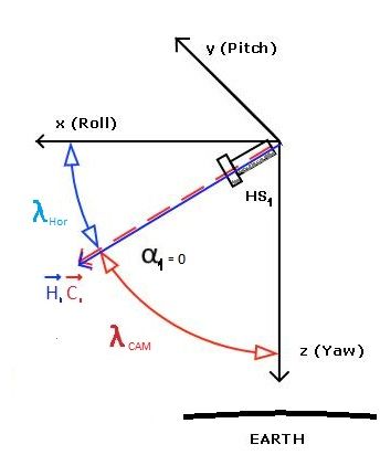
4. RESULTS . . . . . . . . . . . . . . . . . . . . . . . . . . . . . . . . . . . . . . . . 27
 4.1. Free torque motion . . . . . . . . . . . . . . . . . . . . . . . . . . . . . . . . . . 27
 4.2. Nonlinear-linear system comparison . . . . . . . . . . . . . . . . . . . . . . . . 29
 4.3. Camera model . . . . . . . . . . . . . . . . . . . . . . . . . . . . . . . . . . . . 34
  4.3.1. Camera angles . . . . . . . . . . . . . . . . . . . . . . . . . . . . . . . . . . 34
  4.3.2. Cam angles vs Euler angles example . . . . . . . . . . . . . . . . . . . . . . 35
  4.3.3. Initial guess for roll angle IC . . . . . . . . . . . . . . . . . . . . . . . . . . 36
 4.4. Optimization results . . . . . . . . . . . . . . . . . . . . . . . . . . . . . . . . . 39
 4.5. Minimum Mean Square Error variation. Optimization effectiveness range . . . 42
  4.5.1. Time span variation . . . . . . . . . . . . . . . . . . . . . . . . . . . . . . . 42
  4.5.2. Step size variation . . . . . . . . . . . . . . . . . . . . . . . . . . . . . . . . 45
5. CONCLUSIONS . . . . . . . . . . . . . . . . . . . . . . . . . . . . . . . . . . . . 48
6. FUTURE WORK . . . . . . . . . . . . . . . . . . . . . . . . . . . . . . . . . . . . 49
BIBLIOGRAPHY. . . . . . . . . . . . . . . . . . . . . . . . . . . . . . . . . . . . . . 50

                                                                                           viii
LIST OF FIGURES
2.1 Standard CubeSat 3U model . . . . . . . . . . . . . . . . . . . . . . . . 5
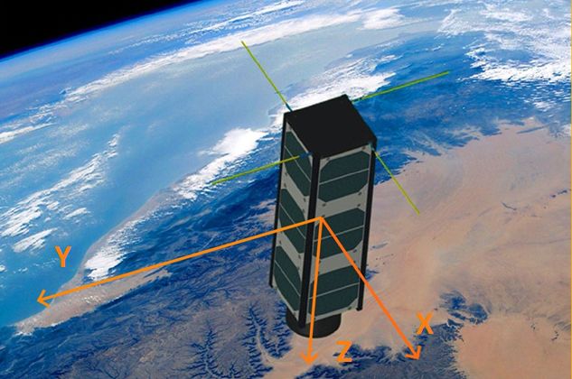
2.2 Example of a static horizon sensor used in the Gemini space capsule.
Taken from [14] . . . . . . . . . . . . . . . . . . . . . . . . . . . . . . . 6
2.3 Attitude sphere representation . . . . . . . . . . . . . . . . . . . . . . . 7
2.4 example of image taken from a infrared detector array . . . . . . . . . . . 7
2.5 scaled satellite’s orbit and significant data . . . . . . . . . . . . . . . . . 9
3.1 Perifocal Coordinate System . . . . . . . . . . . . . . . . . . . . . . . . 10
3.2 Orbit-fixed Coordinate System . . . . . . . . . . . . . . . . . . . . . . . 11
3.3 Body Fixed Coordinate System . . . . . . . . . . . . . . . . . . . . . . . 11
3.4 Definition of the rotation sequence . . . . . . . . . . . . . . . . . . . . . 12
3.5 Visual representation of Euler’s rotational theorem . . . . . . . . . . . . 14
3.6 HS Camera’s orientation angle . . . . . . . . . . . . . . . . . . . . . . . 22
3.7 Sketch of the positioning of the first camera . . . . . . . . . . . . . . . . 23
3.8 Sketch of the positioning of the second camera . . . . . . . . . . . . . . 23
4.1 angular velocity in free torque motion . . . . . . . . . . . . . . . . . . . 27
4.2 Euler angles α and β in free torque motion . . . . . . . . . . . . . . . . . 28
4.3 γ angle in free torque motion . . . . . . . . . . . . . . . . . . . . . . . . 28
4.4 quaternion transformation check in free torque motion . . . . . . . . . . 28
4.5 kinetic energy of the body in free torque motion . . . . . . . . . . . . . . 29
4.6 α and β angles for ω̃=0 . . . . . . . . . . . . . . . . . . . . . . . . . . . 30
4.7 δ perturbation for ω̃=0 . . . . . . . . . . . . . . . . . . . . . . . . . . . 30
4.8 α and β angles for ω̃=10 and non zero IC . . . . . . . . . . . . . . . . . 31
4.9 δ perturbation for ω̃=10 and non zero IC . . . . . . . . . . . . . . . . . . 31
4.10 α and β angles for ω̃=10 and zero IC . . . . . . . . . . . . . . . . . . . . 32
4.11 δ perturbation for ω̃=10 and zero IC . . . . . . . . . . . . . . . . . . . . 32
4.12 α and β angles for ω̃=30 and non zero IC . . . . . . . . . . . . . . . . . 32
4.13 δ perturbation for ω̃=30 and non zero IC . . . . . . . . . . . . . . . . . . 33
x4.14 quaternion squared sum check of the nonlinear system . . . . . . . . . . 33
4.15 kinetic energy of the nonlinear system . . . . . . . . . . . . . . . . . . . 33
4.16 α1 and α2 angles for ω̃=0 . . . . . . . . . . . . . . . . . . . . . . . . . . 34
4.17 α1 and α2 angles for ω̃=10 . . . . . . . . . . . . . . . . . . . . . . . . . 34
4.18 α1 and α2 angles for ω̃=30 . . . . . . . . . . . . . . . . . . . . . . . . . 35
4.19 α1 and α2 vs EA α and β for ω̃=0 . . . . . . . . . . . . . . . . . . . . . . 35
4.20 α1 and α2 vs EA α and β for ω̃=10 . . . . . . . . . . . . . . . . . . . . . 36
4.21 α2 vs α Euler for ω̃=0 zero α0 , non zero β0 . . . . . . . . . . . . . . . . . 36
4.22 α2 vs α Euler for ω̃=0 close to zero α0 , non zero β0 . . . . . . . . . . . . 37
4.23 α2 vs α Euler for ω̃=0 non zero α0 , non zero β0 . . . . . . . . . . . . . . 37
4.24 α2 vs α Euler for ω̃=0 non zero α0 , non zero β0 . . . . . . . . . . . . . . 37
4.25 α2 vs α Euler for ω̃=0 non zero α0 , zero β0 . . . . . . . . . . . . . . . . . 38
4.26 α2 vs α Euler for ω̃=10 zero α0 , zero β0 . . . . . . . . . . . . . . . . . . 38
4.27 α2 vs α Euler for ω̃=10 non zero α0 , zero β0 . . . . . . . . . . . . . . . . 38
4.28 α and β angles for ω̃=0 and non zero IC . . . . . . . . . . . . . . . . . . 39
4.29 δ perturbation for ω̃=0 and non zero IC . . . . . . . . . . . . . . . . . . 39
4.30 α and β angles for ω̃=10 and zero IC . . . . . . . . . . . . . . . . . . . 40
4.31 δ perturbation for ω̃=10 and zero IC . . . . . . . . . . . . . . . . . . . . 40
4.32 α and β angles for ω̃=10 and non zero IC . . . . . . . . . . . . . . . . . 40
4.33 δ perturbation for ω̃=10 and non zero IC . . . . . . . . . . . . . . . . . . 41
4.34 α and β angles for ω̃=30 and non zero IC . . . . . . . . . . . . . . . . . 41
4.35 δ perturbation for ω̃=30 and non zero IC . . . . . . . . . . . . . . . . . . 42
4.36 Cam angles MQE for ω̃=0. Time span variation . . . . . . . . . . . . . . 42
4.37 Euler angles MQE for ω̃=0. Time span variation . . . . . . . . . . . . . . 43
4.38 Cam angles MQE for ω̃=10 non zero IC. Time span variation . . . . . . . 43
4.39 Euler angles MQE for ω̃=10 non zero IC. Time span variation . . . . . . 44
4.40 Cam angles MQE for ω̃=10 close to zero IC. Time span variation . . . . . 44
4.41 Euler angles MQE for ω̃=10 close to zero IC. Time span variation . . . . 45
4.42 Cam angles MQE for ω̃=0. Step size variation . . . . . . . . . . . . . . . 45
4.43 Euler angles MQE for ω̃=0. Step size variation . . . . . . . . . . . . . . 46
4.44 Cam angles MQE for ω̃=10 non zero IC. Step size variation . . . . . . . 46
xi4.45 Euler angles MQE for ω̃=10 non zero IC. Step size variation . . . . . . . 46
4.46 Cam angles MQE for ω̃=10 close to zero IC. Step size variation . . . . . 47
4.47 Euler angles MQE for ω̃=10 close to zero IC. Step size variation . . . . . 47
xiiLIST OF TABLES
xiv1. INTRODUCTION
The idea of outer space has always been an enigma for the humans before the second half
of the XIX century. After the devastating effects of the airplanes during World War I and
II, the population was slowly getting used to fly; kids were raised staring at the blue skies,
probably looking for any of those huge metallic flying machines, the number of which
was increasing rapidly. It was not until October 4th, 1957 that the Russians launched the
first artificial Earth satellite into a low orbit and for just three weeks. This was one of the
milestones achieved by the Soviet Union at the beginning of the Cold War (1947-1991);
however, only 4 years later, Yuri Gagarin surfed the space inside the famous Vostok-
1 for 89 minutes at an approximate speed of 27400 kilometers per hour. Impressive.
The Space Race had begun and USA was not going to step aside. On July 20th, 1969,
after years of hard work, dedication and more importantly, counting on disproportionate
budgets, the Apollo program succeeded and Neil Armstrong became the first human to
step on the moon. That historical fact captivated a very large part of the world’s population
(little over 600 million people watched it), who started to rethink the old idea about the
human inability to navigate through space. The Moon landing was definitely the spark
that initiated the blaze that Space Industry is nowadays.
The space industry has evolved exponentially since then, well known international man-
ufacturers like Airbus, Boeing or Lockheed Martin are playing an important role in the
battle to build (and launch) the most extensive, efficient and profitable satellite network.
In the last years, private companies like Blue Origin or SpaceX have revolutionized the
industry by working on new ways to sell the space business, like for example, private
spaceflights. Earlier this year, in March, SpaceX launched the Crew Dragon Test Flight
to Space Station for NASA [1] which entailed a huge leap towards human spaceflight.
Latest reports show that there are approximately 4987 satellites orbiting the Earth at this
moment [2], and surprisingly, only 1957 of them are active, little less than 40% of them.
Interesting. More than half of them belong to USA and China (830 and 280 respectively)
and 846 were launched for commercial use. Other practices include government, military
and civil which together with the commercial use sum up to 89% of the total use.
One of the most important events that is contributing to the expansion of the satellite net-
work is the proliferation of smallsats. Fast advances in technology, leading to a reliability
and performance increase along with cheaper manufacturing techniques and processes
have facilitated the launch of over 1300 satellites in the last 6 years, being the famous
CubeSat the dominant player with 961 launches between 2012 and 2018 [3]. With an
average mass of 55kg, these little satellites can be launched through LVs (Launching Ve-
hicles) or directly from the International Space Station. Although the mean price for a
LV has not decreased significantly, compared with smallsats, it is expected to do it in
the following years so further and broader constellations of smallsats are forecast for the
1future.
1.1. State of the art
As it was mentioned before, the advances in the vast majority of the components of the
smallsats have promoted its use to the extent that almost any university, research center or
individual, with little investment, is able to launch one. Minimum investment have been
about $150,000 [4] ($50,000 for manufacturing and $100,000 for launching) which makes
it quite affordable for small users of both commercial and scientific areas. Development
of lighter materials for the satellite’s structure, more efficient solar panels and batteries for
the electrical power system and improved electronics for attitude determination, control
and general onboard computing are just few examples that show the significant moment
this sector is living.
Despite CubeSats were initially thought to be used in a low orbit environment, between
those 961 launched there are two examples of a more ambitious application [5]: the inter-
planetary mission. The success of these two CubeSats, which accompanied the InSight
on its mission to Mars, was a clear proof of the place that CubeSats deserve within the
future of space exploration.
However, among all the CubeSat systems, the one concerning this work is the attitude
determination and control system (ADCS), and more precisely, the first one. Different
sensors are used for attitude determination, such as Sun sensors, star trackers, magne-
tometers and horizon sensors, but it is really the latter the one that is able to provide nearly
uninterrupted fine attitude knowledge [6]. The previous fact along with an inexpensive
manufacturing and improvements in the infrared detection technology had considerably
contributed to their implementation in the CubeSats, accomplishing a 1σ nadir estimation
error of less than 0.2 degrees.
1.2. Socio-economic impact
The development of cheaper and more efficient smallsats is causing the satellite manufac-
turing and launch industry to grow year after year. The global market revenues where of
$277M in 2018 [7], of which half of them were related to satellite services like mobile
and broadband or TV and transponder leasing. However, the largest increase in revenues
were found in the launch industry, with an increment of 34% in 2018.
Related to the communications and broadcasting industry, OneWeb Satellites, the joint
venture between Airbus and OneWeb, has recently launched its first batch of 5G satellites
that will provide fast internet access everywhere in the Earth [8]. The company’s plan is
to had deployed a total of 650-satellites by 2020, which directly competes with SpaceX’s
Starlink project of putting up 12000 satellites, being able to go live by summer 2020 once
800 of them have been launched.
2Nonetheless, as it is known, not everything related with progress is positive. Space debris
is a problem that could create serious consequences in the future. First scenario, caused
by debris reentring the Earth’s atmosphere, like the Tiangong-1 case, where even being
an uncontrolled reentry, it was completely expected and monitored [9]. Second scenario
and more important, the density of the objects orbiting the Earth. Companies providing
satellite constellations should also be able to guarantee the proper elimination of the mal-
functioning or inactive old satellites in order to avoid the disastrous Kessler effect [10].
1.3. Motivation
The exponential growth that the space, and in particular, the satellite industry is experi-
encing is highly interesting. It brings the opportunity to develop new skills related to a
topic that means present and future. Personally, I think is quite a challenge to develop a
code that its meant to simulate a real situation that is to be happening at an altitude of
hundreds or thousands of kilometers. Besides, as an engineer about to finish his degree, I
find it quite satisfying to end my career applying the tools acquired at university to write
an algorithm capable of solving a certain problem and subsequently, interpreting those
results to give them validity. Professionally, I believe that earning some experience about
space-related topics will always bring good chances to aim for a good job offers.
1.4. Objectives
The aim of this work is to develop an optimization algorithm using MATLAB that is able
to determine the attitude of a slender body satellite when this is close to Earth-pointing
nominal conditions. The algorithm uses exclusively as inputs the simulated data extracted
from the implementation of two single horizon sensors.
1.5. Outline
In chapter 1 an introduction to the topic of the work is included. State of the Art, socio-
economic impact, motivation of the project, main objectives and project outline are also
included
Chapter 2 includes the description of the model and the assumptions stated. Satellite’s
body and orbit are defined as well as a brief introduction to the horizon sensor operation.
Chapter 3 exposes all the mathematical considerations of the problem and the strategy to
solve it. A complete description of the algorithm operation is also included.
Chapter 4 contains the analysis and interpretation of the results of the different simulations
carried out. Besides, results showing the accuracy of the algorithm in several ranges of
study are also included.
3Chapter 5 includes the conclusions of the work, focusing on the initial assumptions and
how they could differ from reality.
Chapter 6 includes a set of ideas for a future work that increase the boundaries of the
problem in order to provide a more realistic approach of it.
42. MODEL DESCRIPTION
In this chapter, the general characteristics of the satellite’s body and orbit will be de-
scribed. Besides, the basic operation of the horizon sensor simulated in the work is ex-
plained.
2.1. Satellite’s Model
The satellite’s body selected for this work was chosen based on the CubeSat 3U standard
model [11]. However it has been modified in order to obtain a true slender body vehicle.
The following properties are listed:
• Dimensions: x=0.1m y=0.1m z=1.55m (x:length y:width z:height)
• Mass: 1.33 kg
Iz
• I x = Iy = 0.266 kgm2 Iz = 0.0022 kgm2 ≈ 120.9
Ix
In figure 2.1 is shown the standard version of a CubeSat 3U in which the model is based.
As it was said before the satellite’s body is assumed to be slender so its height has been
incremented substantially. Is not in the scope of this work to analyze the structural impli-
cations of such a slender body, but it is sure that they must be studied carefully.
Fig. 2.1. Standard CubeSat 3U model
5In addition, figure 2.1 shows the possible locations of the different attitude determination
sensors, such as star trackers, Sun sensors and horizon sensors. Another example of a 3U
CubeSat satellite model and its characterization can be found on [12]. However, this work
is exclusively focused on the operation of the horizon sensor, in this way in section 3.6
the position and collocation of the cameras is completely explained.
2.2. Horizon Sensor
Earth horizon sensors picture the proximity of the Earth horizon (also called limb) to lo-
cate the non-thermal airglow emissions. They detect the interface between the Earth’s
edge and the space background [13]. Two main categories of horizon sensors can be
found, scanning and static. Scanning type scans the Earth pursuing the horizon cross-
ings and measuring the time span between horizon crossings. In static type however, the
picture of the horizon is captured onto an infrared detector array so it allows the limb to
be determined from the image. The range or field of view of a static horizon sensor is
sometimes larger than the complete Earth’s horizon.
Fig. 2.2. Example of a static horizon sensor used in the Gemini space capsule. Taken from [14]
2.2.1. Information obtained from one horizon sensor
The document [15] is going to be used as reference to explain the mathematical aspects
of the operation of the horizon sensor. First of all, the basic geometry of the problem is
pictured in figure 2.3, where the sphere of attitude of the satellite is draw,
6Fig. 2.3. Attitude sphere representation
where z0 is the document’s orbit fixed Z axis, z is the body fixed Z axis, ⃗b is the sweep
⃗ is the horizon vector as
vector, usually linked to z, ⃗c is the camera’s line of vision and H
seen by the camera. The latter is defined as the vector pointing to the intersection of the
plane formed by vectors ⃗b and ⃗c with the projection of the Earth’s horizon over the sphere
of attitude, in section 3.6 is explain in more detail. The angle of interest is the one formed
⃗ α.
by the vectors ⃗c and H,
The final step is obtaining the angle α from the infrared detector array image as follows
Fig. 2.4. example of image taken from a infrared detector array
from figure 2.4 two angles are defined, the inclination angle δ and α. The following
equations are obtained taking into account the illuminated areas on left and right cells and
7the total height h and width w of them.
wx2 w2 2
( )
2 tanδ
Larea = wx − − 2 h − 2hx + x (2.1)
2h h 2
wx2 w2 2 tanδ
Rarea = + 2x (2.2)
2h h 2
Solving for tanδ in both equations and equating them, the following quadratic equation is
obtained ( )
wh 2
Rarea + Larea − x − 2hRarea x + Rarea h2 = 0 (2.3)
2
Solving for x and using the hypothesis of a small δ to discriminate one of the two solutions
[15], the angle x or α is obtained.
It is important to remark that the information retrieved from the operation of one sensor is
insufficient to determine the satellite’s attitude with exactness. The precision in the calcu-
lation of the angle δ is low. In consequence, for a complete, more accurate determination
of the attitude, two sensors will be used.
2.3. Satellite’s Orbit
In order to simplify the calculations, the selected orbit is perfectly circular. Main charac-
teristics are written below
• Type: circular
• Altitude: 998 [km] Low Earth Orbit (LEO)
• Angular velocity: Ω=0.001 [rad/s]
• Period: 6283.19 [s] ≈ 1.75 [h]
In order to get a visual reference, the following plot shows the top view representation of
the orbit in a random instant in time.
8Fig. 2.5. scaled satellite’s orbit and significant data
93. METHODOLOGY
The physical model proposed by this work is a slender body satellite orbiting around the
Earth by the effect of the gravity gradient. In this chapter, the problem will be completely
defined and both physical and mathematical aspects will be exposed following the same
criteria as [16] and [15]. All the assumptions stated for the model and its expected limita-
tions will described as well. Finally, a strategy to solve it will be proposed.
3.1. Coordinate systems
Firstly, the coordinate systems used for determining the rotation of the satellite will be
defined following the same principles as [16].
3.1.1. Perifocal Coordinate System
This coordinate system is very close to be inertial, which will be the base for our descrip-
tion of the Euler equations later. The origin is placed at the Earth’s center, the Y axis is
perpendicular to the orbits plane, the Z axis is directed to the perigee and finally, X is
defined following the right hand’s rule with Y and Z. This system of coordinates is found
below:
Fig. 3.1. Perifocal Coordinate System
The system is considered to be inertial although the orbit is not fixed, as it experiences
a small precession. This effect will be neglected for the sake of simplicity and due to
the fact that is a much slower movement compared to the ones studied in this work. The
unitary vectors are I⃗0 , J⃗0 and K⃗0 .
103.1.2. Orbit Fixed Coordinate System
The orbit is perfectly circular with constant angular velocity so the attitude of the satellite
is defined with respect to this system. The Z axis is always pointing to the center of the
Earth, the X axis follows the same path as the velocity vector of the satellite and the Y
vector just the resultant of the natural vector product between the previous two. This
system is illustrated below:
Fig. 3.2. Orbit-fixed Coordinate System
It should be noted that, as this system is rotating at a constant angular velocity, it is
considered non-inertial. The unitary vectors are defined as ⃗I, J⃗ and K.
⃗
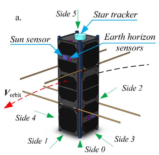
3.1.3. Body Fixed Coordinate System
This is the system used to project the equations of motion. The origin coincides with the
center of mass of the satellite, the Z axis is aligned with the lowest moment of inertia and
X and Y axes are aligned with the other two principal moments of inertia. The nominal
conditions of this system match the orbit fixed system. The picture below shows the body
fixed frame in a CubeSat 3U.
Fig. 3.3. Body Fixed Coordinate System
11The unitary vectors of this coordinate system are ⃗i, ⃗j and ⃗k.
3.2. Attitude Representation
The attitude is defined as the orientation of the body fix frame with respect to the orbit-
fixed one. For a proper parametrization the selected Euler sequence is 2-1-3 (Y-X-Z), also
called Tait-Bryan or Cardan Angles. These rotations are physically represented below:
Fig. 3.4. Definition of the rotation sequence
The first rotation about the YA axis is represented by the angle β, the second one, about
the intermediate axis XB′ , by the angle α and last one, about axis ZB′′ by the angle γ. Note
that the axes YA and ZB′′ belong to the orbit fixed and body fixed frames respectively.
Now, the rotation matrix of the transformation needs to be obtained. This is simply done
multiplying the matrices of each rotation sequence as follows:
⎢⎢⎢⃗i ⎥⎥⎥ ⎢ ⃗I ⎥
⎡ ⎤ ⎡ ⎤
⎢⎢⎢ ⎥⎥⎥ [ ] ⎢⎢⎢⎢⎢ ⎥⎥⎥⎥⎥
⎢⎢⎢⃗j⎥⎥⎥ = R ⎢⎢⎢ J⃗⎥⎥⎥ (3.1)
⃗k ⃗
⎢⎣ ⎥⎦ ⎢⎣ ⎥⎦
K
⎢⎢⎢⃗i ⎥⎥⎥ ⎢⎢⎢ ⃗I ⎥⎥⎥
⎡ ⎤ ⎡ ⎤
⎢⎢⎢⎢⃗⎥⎥⎥⎥
⎢⎢⎢ j⎥⎥⎥ = R(γ) R(α) R(β) ⎢⎢⎢⎢⎢ J⃗⎥⎥⎥⎥⎥
[ ] [ ] [ ] ⎢⎢ ⎥⎥
(3.2)
⎣⃗ ⎦ ⎣⃗⎦
k K
⎢⎢⎢⃗i ⎥⎥⎥ ⎢⎢⎢ c(γ) s(γ) 0⎥⎥⎥ ⎢⎢⎢1 0 ⎥⎥⎥ ⎢⎢⎢c(β) 0 −s(β)⎥⎥⎥ ⎢⎢⎢ ⃗I ⎥⎥⎥
⎡ ⎤ ⎡ ⎤⎡ ⎤⎡ ⎤⎡ ⎤
0
⎢⎢⎢⎢⃗⎥⎥⎥⎥ ⎢⎢⎢⎢
⎢⎢⎢ j⎥⎥⎥ = ⎢⎢⎢−s(γ) c(γ) 0⎥⎥⎥⎥⎥ ⎢⎢⎢⎢⎢0 c(α) s(α)⎥⎥⎥⎥⎥ ⎢⎢⎢⎢⎢ 0) 1 0 ⎥⎥⎥⎥ ⎢⎢⎢⎢ J⃗⎥⎥⎥⎥
⎥⎥ ⎢⎢ ⎥⎥ ⎢⎢ ⎥⎥ ⎢⎢ ⎥⎥
(3.3)
⎣⃗ ⎦ ⎣ ⃗
⎥⎦ ⎢⎣ ⎥⎦
k 0 0 1 0 −s(α) c(α) s(β) 0 c(β) K
⎦⎣ ⎦⎣
So the matrix multiplication brings:
⎢⎢⎢ c(γ)c(β) + s(γ)s(α)s(β) s(γ)c(α) −s(β)c(γ) + s(γ)s(α)c(β)⎥⎥⎥
⎡ ⎤
[ ] ⎢⎢
R = ⎢⎢⎢⎢−s(γ)c(β) + c(γ)s(α)s(β) c(γ)c(α) s(γ)s(β) + c(γ)s(α)c(β) ⎥⎥⎥⎥
⎥⎥
(3.4)
⎢⎣ ⎥⎦
s(β)c(α) −s(α) c(α)c(β)
12It should be noted that if the reverse operation wants to be performed, BFaxes → OFaxes ,
it will be enough to calculate the inverse of the matrix 3.4
⎢⎢⎢ ⃗I ⎥⎥⎥ ⎢⎢⃗i ⎥⎥⎥
⎡ ⎤ ⎡ ⎤
−1 ⎢
⎢⎢⎢ J⃗⎥⎥⎥ = R ⎢⎢⎢⎢⎢⃗j⎥⎥⎥⎥⎥
⎢⎢⎢ ⎥⎥⎥ [ ] ⎢ ⎥
(3.5)
⃗ ⃗k
⎢⎣ ⎥⎦ ⎢⎣ ⎥⎦
K
3.2.1. Quaternions
The representation of the attitude of an object, in this case the satellite, using Euler angles
is simple to develop and visualize but it could imply a major drawback for some reasons.
The first one, Euler angles are computationally more intense compared to quaternions and
second and more important, the singularity problem that occurs with certain combinations
that cause the famous Gimbal Lock.
The quaternion representation method is based on Euler’s theorem which states that the
relative orientation of two coordinate systems can be defined by only one rotation about a
fixed axis. With this idea in mind, the implementation of the rotation kinematics is done
using this number system.
A quick overview about quaternion operation will be done, showing the most important
equations but in order to check more information about their properties and significance,
please refer to [17] and [18].
The quaternion below represents a coordinate transformation between 2 systems
⃗ = Q s + Q1⃗i + Q2 ⃗j + Q3⃗k
Q (3.6)
where the included vectors are unit vectors. The previous expression is mathematically
equivalent to ⎡ ⎤
⎢⎢⎢ Q s ⎥⎥⎥
⎢⎢⎢⎢ ⎥⎥⎥⎥ ⎡⎢ θ
⎤
⃗ ⎢⎢⎢Q1 ⎥⎥⎥ ⎢⎢⎢ cos( 2 ) ⎥⎥⎥⎥
Q = ⎢⎢ ⎥⎥ = ⎣ (3.7)
⎢⎢⎢Q2 ⎥⎥⎥ ∥⃗e∥sin( 2θ )
⎦
⎣⎢ ⎦⎥
Q3
where ∥⃗e∥ is the normalized axis of rotation and θ is the transformation angle, the picture
below explains this concept more clearly
13Fig. 3.5. Visual representation of Euler’s rotational theorem
In order to obtain the quaternions from Euler angles, the little algorithm shown in [17] is
used. Four initial values of the quaternion’s components are obtained through the values
of the rotational matrix 3.4 and implementing a short conditional statement the true values
are defined.
Once the four values are set, the system of kinematic equations that relate the angular
velocity and the quaternion with the derivative of the latter. It is a system of four first
order ODEs in the form
⎡ ⎤ ⎡ ⎤⎡ ⎤
⎢⎢⎢Q̇1 ⎥⎥⎥ ⎢⎢⎢ 0 −ω x −ωy −ωz ⎥⎥⎥ ⎢⎢⎢Q1 ⎥⎥⎥
⎢⎢⎢Q̇2 ⎥⎥⎥ 1 ⎢⎢⎢⎢⎢ω x 0 ωz −ωy ⎥⎥⎥⎥ ⎢⎢⎢⎢Q2 ⎥⎥⎥⎥
⎢⎢⎢ ⎥⎥⎥ ⎢ ⎥⎥ ⎢⎢ ⎥⎥
⎢⎢⎢⎢ ⎥⎥⎥⎥ = ⎢⎢⎢⎢ (3.8)
⎢⎢⎢Q̇3 ⎥⎥⎥ 2 ⎢⎢⎢ωy −ωz ω x ⎥⎥⎥⎥ ⎢⎢⎢⎢Q3 ⎥⎥⎥⎥
⎥⎥ ⎢⎢ ⎥⎥
0
ωz ωy −ω x 0 Q4
⎥⎦ ⎢⎣ ⎥⎦
Q̇4
⎣ ⎦ ⎣
For the inverse operation, the equivalent of the rotational matrix defined in quaternion
form is
⎢⎢⎢Q1 + Q22 − Q23 − Q24 2(Q2 Q3 + Q4 Q1 )
⎡ 2 ⎤
[ ] ⎢⎢ 2(Q 2 Q 4 − Q 3 Q 1 ) ⎥⎥⎥
RQ = ⎢⎢⎢⎢ 2(Q2 Q3 − Q4 Q1 ) Q21 − Q22 + Q23 − Q24 2(Q3 Q4 + Q2 Q1 ) ⎥⎥⎥⎥
⎥⎥
(3.9)
2(Q2 Q4 + Q3 Q1 ) 2(Q3 Q4 − Q2 Q1 ) Q1 − Q2 − Q3 + Q4
⎣⎢ 2 2 2 2⎦
⎥
and the corresponding Euler angles definitions are simply obtained from the relationship
with the rotational matrix 3.4 as
( )
α = asin − RQ,32 (3.10)
( )
RQ,31
β = atan (3.11)
RQ,33
( )
RQ,12
γ = atan (3.12)
RQ,22
14Last but not least, an easy way to check if the quaternions are being calculated correctly,
is to perform the squared sum of its components.
Q21 + Q22 + Q23 + Q24 = 1 (3.13)
As they are normalized vectors, the theoretical sum of its components should be 1. This
check is implemented in the code to monitor the error of the conversion.
3.3. Equations of Motion
The Euler equations of motion describe the rotation of a rigid body using a rotating ref-
erence frame with its axes fixed to the body and aligned to the body’s principal axes of
inertia. They have the form:
I x ω̇ x + (Iz − Iy )ωy ωz = M x (3.14)
Iy ω̇y + (I x − Iz )ω x ωz = My (3.15)
Iz ω̇z + (Iy − I x )ω x ωy = Mz (3.16)
Where the angular velocity terms and their derivatives are written with respect to the
inertial reference frame shown in section 3.1.1. The terms I x , Iy and Iz are the principal
axes of inertia and M x , My and Mz the applied torques. All of them will be projected in
body fixed coordinates.
3.3.1. Applied Torques
This work is focused on the disturbances occurring when the satellite is under the effect
of the Earth’s gravity gradient, hence, this torque will be the only one applied.
It is known that the point value of the gravity decreases with the square of the distance of
that point to the center of the Earth. Being this satellite a slender body, the effect is quite
important and should be carefully taken into account and later studied.
Starting with the description of the differential of the force, written
⃗ + ⃗ρ)
µ(R
d F⃗ = − dm (3.17)
⃗ + ⃗ρ∥3
∥R
Here, µ is the product of the universal gravitational constant and the mass of the Earth,
⃗ is the vector of the center of mass of the satellite in orbit
adding up to µ = 3.9858 · 1014 . R
fixed frame and ⃗ρ is the vector of each differential of mass in body fixed axes. Integrating
∫ ⃗
⃗ρ ∧ R
M⃗gg = −µ dm (3.18)
V ⃗ + ⃗ρ∥3
∥R
15Expressing again each of the terms in body fixed frame
⎡ ⎤
⎢⎢⎢−R13 R⎥⎥⎥
⃗ BF = ⎢⎢⎢⎢−R23 R⎥⎥⎥⎥
⎢ ⎥
R ⎢⎣⎢ ⎥⎦⎥ (3.19)
−R33 R
⎡ ⎤
⎢⎢⎢ x⎥⎥⎥
⃗ρBF = ⎢⎢⎢⎢y⎥⎥⎥⎥
⎢⎢ ⎥⎥
(3.20)
⎣⎢ ⎦⎥
z
To avoid any confusion, it should be remarked the differences between the term R referring
to the position of the center of mass of the satellite and Ri j , being i the row position and
j the column position, referring to each of the terms of the rotational matrix described in
equation 3.4.
Assuming that ρFor the angular velocity of the satellite with respect to orbit fixed axes, using the notation
of 3.4 as follows:
ω⃗BF = β̇ J⃗ + α̇X⃗B′ + γ̇⃗j (3.27)
the expression of ω⃗BF , applying the vector transformation for J⃗ and X⃗B′ results
⎢⎢⎢ p⎥⎥⎥ ⎢⎢⎢β̇cos(α)sin(γ) + α̇cos(γ)⎥⎥⎥
⎡ ⎤ ⎡ ⎤
ω⃗BF = ⎢⎢⎢⎢ q ⎥⎥⎥⎥ = ⎢⎢⎢⎢β̇cos(α)cos(γ) − α̇sin(γ)⎥⎥⎥⎥
⎢⎢ ⎥⎥ ⎢⎢ ⎥⎥
(3.28)
γ̇ − β̇sin(α)
⎣⎢ ⎦⎥ ⎣⎢ ⎦⎥
r
so the final expression of the angular velocity ω⃗0 and its derivative in body fixed frame is:
ω x = p − ΩR12 ω̇ x = ṗ − ΩR˙12 (3.29)
ωy = q − ΩR22 ω̇y = q̇ − ΩR˙22 (3.30)
ωz = r − ΩR32 ω̇z = ṙ − ΩR˙32 (3.31)
It is very important to remark that the Coriolis terms of the derivatives have been canceled
due to the definition of a derivative of a vector with respect to a non-inertial reference
frame. Coriolis’ theorem states that the derivative of a vector in a non-inertial reference
frame is given by the derivative of its components as seen by the rotating frame, plus an
additional term given by the vector product between the angular velocity of the rotating
frame and the vector itself. As it is shown below the components of the vector product
are exactly the same, so the second term below is cancelled.
dω⃗0 dω⃗0 dω⃗0
[ ] [ ]
= +ω⃗0∧ ω⃗0 =
(3.32)
dt dt BF dt BF
3.4. Final expression of Euler Equations
Substituting all the previous terms into equations 3.14, 3.15 and 3.16, the final set of
equations of motion are read
I x ṗ+(Iz −Iy )qr−I x ΩR˙12 −(Iz −Iy )(ΩqR32 +ΩrR22 )+R32 R22 Ω2 (Iz −Iy ) = −3Ω2 R23 R33 (Iy −Iz )
(3.33)
Iy q̇+(I x −Iz )pr−Iy ΩR˙22 −(I x −Iz )(ΩpR32 +ΩrR12 )+R12 R32 Ω2 (I x −Iz ) = −3Ω2 R13 R33 (Iy −Iz )
(3.34)
Iz ṙ+(Iy −I x )pq−Iz ΩR˙32 −(Iy −I x )(ΩqR12 +ΩpR22 )+R12 R22 Ω2 (Iy −I x ) = −3Ω2 R13 R23 (Iy −Iz )
(3.35)
17and the only terms that have not been defined are the derivatives of the rotation matrix
components
R˙12 = −α̇sin(α)sin(γ) + γ̇cos(α)cos(γ) (3.36)
R˙22 = −α̇sin(α)cos(γ) − γ̇cos(α)sin(γ) (3.37)
R˙32 = −α̇cos(α) (3.38)
The integration of the first order ODEs 3.33, 3.34 and 3.35 together with kinematic equa-
tions in quaternion form 3.8 is performed via Simulink (MATLAB), applying the numeri-
cal methods that ode45 typically uses. Simulink integrators have as inputs a set of 6 initial
conditions
⎢⎢⎢α0 ⎥⎥⎥
⎡ ⎤
⎢⎢⎢ β0 ⎥⎥⎥
⎢⎢⎢ ⎥⎥⎥
⃗ = ⎢⎢⎢⎢ γ0 ⎥⎥⎥⎥
⎢⎢⎢ ⎥⎥⎥
⎢ ⎥
I.C ⎢⎢⎢ p0 ⎥⎥⎥ (3.39)
⎢⎢⎢ ⎥⎥⎥
⎢⎢⎢ q ⎥⎥⎥
⎢⎢⎣ 0 ⎥⎥⎦
r0
3.5. Linearization and analytical solution
In order to create a functional algorithm, it is necessary to obtain the simplified analytical
solution of the previously defined non-linear Euler equations. As the previous develop-
ment, this will be done by means of [16].
3.5.1. Linearization
The main hypothesis proposed to linearize the equations is within the description of the
problem. As this work is exclusively focus on the small perturbations from the satellite’s
nominal position due to the gravity gradient and the slender body condition, the assump-
tion of small roll and pitch angles (α, β ≪ 1) is expected to bring accurate results.
In principle, the angular velocity r or spin is not negligible and in fact, will be much
larger than the orbit’s angular velocity Ω. This condition will cause the angle γ to reach
any value from 0 to 2π. However, in the following pages, a way to linearize the yaw angle
is introduced as well.
Linearization of the equations follows these assumptions:
• sin(α), sin(β) ≈ α, β
• cos(α), cos(β) ≈ 1, 1
• sin(α)·sin(β) ≈ 0
18• α̇ · β̇ ≈ 0
And applying one the very first conditions stated in chapter ??, I x = Iy , the following set
of linearized equations is
I x (β̈sinγ+ α̈cosγ)+Iz β̇γ̇cosγ−Iz α̇γ̇sinγ = 4Ω2 (Iz −I x )αcosγ+Iz Ωγ̇cosγ+3Ω2 (Iz −I x )βsinγ
(3.40)
I x (β̈cosγ−α̈sinγ)−Iz β̇γ̇sinγ−Iz α̇γ̇cosγ = −4Ω2 (Iz −I x )αsinγ−Iz Ωγ̇sinγ+3Ω2 (Iz −I x )βcosγ
(3.41)
γ̈ = −Ωα̇ (3.42)
This system of equations is further simplified substituting eqs 3.40 and 3.41 by a linear
combination of both, resulting in
I x β̈ − Iz α̇γ̇ + 3Ω2 (I x − Iz )β = 0 (3.43)
I x α̈ + Iz β̇γ̇ + 4Ω2 (I x − Iz )α − Iz Ωγ̇ = 0 (3.44)
Following as well the idea of [16], γ was not able to be linearized due to its full range of
values. Nonetheless, taking advantage of the fact of a high spin velocity in comparison
with Ω, from now on, the spin will be denoted by w s .
The procedure shows that the yaw angle can be decomposed as the sum of a big term and
a small one
γ = wst + δ (3.45)
with δ ≪ w s t. Then we take derivatives of equation 3.45
γ̇ = w s + δ̇ (3.46)
γ̈ = δ̈ (3.47)
and substituting in 3.42
δ̈ = −Ωα̇ (3.48)
and integrating again once,
δ̇ = −Ωα + Ωα0 (3.49)
substituting equations 3.46 and 3.49 into 3.43 and 3.44 and neglecting second order terms
again, the equations become
I x β̈ − Iz α̇w s + 3Ω2 (I x − Iz )β = 0 (3.50)
19( )
3
I x α̈ + Iz β̇w s + 4Ω I x − Iz α − Iz Ωw s = 0
2
(3.51)
4
δ̇ = −Ωα + Ωα0 (3.52)
The very last step before starting to discuss it analytically is to adimensionalize it. The
following adimensional parameters are defined:
Iz
I=
Ix
ws
ω̃ =
Ω
τ = Ωt
and dividing the first two equations by Ω2 and I x and the last one just by Ω, the final
adimensional linearized equations are
β′′ − Iα′ ω̃ + 3(1 − I)β = 0 (3.53)
( )
3
α + Iβ ω̃ + 4 1 − I α − I ω̃ = 0
′′ ′
(3.54)
4
δ′ = −α + α0 (3.55)
3.5.2. Analytical Solution
It can be seen that the first two equations 3.53 and 3.54 are decoupled from the third one.
So the system can be solved using the first two equations and then apply the results to the
third one in order to obtain the third angle.
The whole process to obtain the solution does not present much complexity but it could
result long and tedious. For those interested, the full development is found again within
article [16].
The important points to take into account in order to correctly study the behavior in time
of the system start with the particular solutions of equations 3.53 and 3.54,
βP = 0 (3.56)
I
αP = ω̃ (3.57)
4 − 3I
The particular solution αP is also called Roll-bias. Applying the condition of slender body
I ≪ 1, automatically, αP ≪ 1
20From the characteristic equation of the system,
σ4 + (7 − 6I + I 2 ω̃2 )σ2 + 3(1 − I)(4 − 3I) = 0 (3.58)
the frequencies σi are calculated
σ1,3 ≈ ±2i (3.59)
√
σ2,4 ≈ ± 3i (3.60)
It can be seen that both frequencies are pure frequencies (no real part) but slightly different
in value. It is determined that the system is stable as long as the condition I ≪ 1 remains,
independently of the value of the adimensional spin ω̃
Finally the analytical solution of the system is
I
α = C1 S 21 cosσ1 τ + C2 T 21 sinσ1 τ + C3 S 22 cosσ2 τ + C4 T 22 sinσ2 τ + ω̃ (3.61)
4 − 3I
β = C1 S 11 cosσ1 τ + C2 T 11 sinσ1 τ + C3 S 12 cosσ2 τ + C4 T 12 sinσ2 τ (3.62)
( ) ( ) ( ) ( )
S 21 T 21 S 22 T 22 I
δ = C1 − sinσ1 τ+C2 cosσ1 τ+C3 − sinσ2 τ+C4 cosσ2 τ−ω̃ τ+α0 τ
σ1 σ1 σ2 σ2 4 − 3I
(3.63)
Only the imaginary part of σi is taken in order to solve the equations. Moreover, T i j and
S i j are defined as
S i j = Re[ai j ] + Im[ai j ] (3.64)
T i j = Re[ai j ] − Im[ai j ] (3.65)
and being ai j the eigenvectors of the problem, whose value has been approximated fol-
lowing the assumptions to
⎡ ⎤ ⎡ √1−I−I 2 ω̃2 ⎤
⎢⎢⎢a11 ⎥⎥⎥ ⎢⎢⎢ √ i⎥⎥⎥⎥
⎢⎣ ⎥⎦ = ⎢⎢⎣ 3I ω̃ ⎥⎦ (3.66)
a21 1
⎡ ⎤ ⎡ ⎤
⎢⎢⎢a12 ⎥⎥⎥ ⎢⎢⎢ 1
⎢⎣ ⎥⎦ = ⎢⎢⎣ √1−0.75I+I 2 ω̃2 ⎥⎥⎥⎦
⎥⎥
(3.67)
a22 2I ω̃
i
and last, the constants C1 , C2 , C3 and C4 which depend on the initial conditions α0 , β0 , α˙0
and β˙0
β0 S 21 − α0 S 11 + αP S 11
C3 = (3.68)
S 12 S 21 − S 22 S 11
21β0 − C3 S 12
C1 = (3.69)
S 11
β˙0 T 21 − α˙0 T 11
C4 = (3.70)
σ2 (T 12 T 21 − T 22 T 11 )
β˙0 − C4 T 12 σ2
C2 = (3.71)
σ1 T 11
3.6. Horizon Sensor angles
Once the analytical solution is ready to be implemented, the last part before developing
the algorithm is to extract the horizon sensor angles. This will be done introducing the
Euler angles obtained from the simulation in the equations that will be deduced below.
The orientation angle of the cameras within the horizon sensors is chosen solving the
following simple trigonometric problem,
Fig. 3.6. HS Camera’s orientation angle
From there, using the particular data of the mission, the angle is obtained
( )
REarth
λhor = acos ≈ 30.05o (3.72)
REarth + h sat
From figure 3.6 the orientation of horizon vector explained in chapter ?? is defined.
22Following the guidelines of [15] but applying some changes in the orientation of the
reference frames shown in the document, the system of equations that provide the horizon
sensor angles are going to be deduced. Before doing so, in order to provide a proper
visualization of the problem. Using the information of chapter ??, the following pair
of schemes, showing the orbit fixed and body fixed coordinate systems as well as the
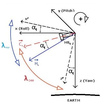
direction vector of the cameras. The sketch made for the first camera, or cam-1,
(a) cam-1 initial position for β0 = 0 (b) cam-1 initial position for β0 , 0
Fig. 3.7. Sketch of the positioning of the first camera
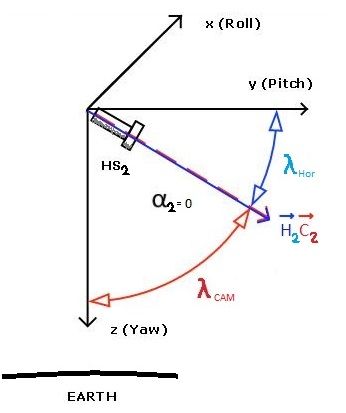
and for the second camera, or cam-2,
(a) cam-2 initial position for α0 = 0 (b) cam-2 initial position for α0 , 0
Fig. 3.8. Sketch of the positioning of the second camera
23By definition, the angle λcam is fixed and it reads
π
λcam = − λhor (3.73)
2
Once the problem is visualized, it is not complex to obtain the equations relating the
camera angles and the Euler angles. Taking into account the definition of the horizon
vectors H⃗1 and H⃗2 from figures 3.7 and 3.8. Expressed in body fixed frame,
H⃗1 = sin(λcam − α1 )⃗i + 0⃗j + cos(λcam − α1 )⃗k (3.74)
H⃗2 = 0⃗i + sin(λcam − α2 )⃗j + cos(λcam − α2 )⃗k (3.75)
Equations 3.74 and 3.75 show that α1 , the angle swept by cam-1 is positive when β0 is
also positive. However, the sense of rotation of the roll axis will bring a negative cam-2
angle when α0 > 0
Now, the rotation matrix 3.4 is used to transform the horizon vectors to orbit fixed frame
as,
⎡ ⎤ ⎡ ⎤
⎢⎢⎢H1,x ⎥⎥⎥
[ ]−1 ⎢⎢⎢⎢h1,x ⎥⎥⎥⎥
⎢ ⎥
⎢⎢⎢ H1,y ⎥⎥⎥ = R ⎢⎢⎢⎢h1,y ⎥⎥⎥⎥
⎢⎢⎢ ⎥⎥⎥
(3.76)
⎢⎣ ⎥⎦ ⎢⎣ ⎥⎦
H1,z OF h1,z BF
⎡ ⎤ ⎡ ⎤
⎢⎢⎢H2,x ⎥⎥⎥
[ ]−1 ⎢⎢⎢⎢h2,x ⎥⎥⎥⎥
⎢ ⎥
⎢⎢⎢ H2,y ⎥⎥⎥ = R ⎢⎢⎢⎢h2,y ⎥⎥⎥⎥
⎢⎢⎢ ⎥⎥⎥
(3.77)
⎢⎣ ⎥⎦ ⎢⎣ ⎥⎦
H2,z OF h2,z BF
The last components of each of the vectors calculated, H1,z and H2,z are known (they are
the same indeed H1,z = H2,z ), so their two expressions are formulated as follows
R13 sin(λcam − α1 ) + R33 cos(λcam − α1 ) = H1,z ≈ sin(30.05) (3.78)
R23 sin(λcam − α2 ) + R33 cos(λcam − α2 ) = H2,z ≈ sin(30.05) (3.79)
Using some trigonometric identities (angle difference and pythagorean) a set of two quadratic
equations is obtained, ready to be solved,
(A2 + B2 )sinα1 2 − 2AH1,z sinα1 + (H1,z
2
− B2 ) = 0 (3.80)
(A2 2 + B2 )sinα2 2 − 2A2 H2,z sinα2 + (H2,z
2
− B2 ) = 0 (3.81)
24where the terms A, A2 and B are defined as
A = R13 sinλcam + R33 cosλcam (3.82)
A2 = R23 sinλcam + R33 cosλcam (3.83)
B = R33 (3.84)
With this solution, the camera angles can be obtained using the data coming from the
simulation, that is to say, the horizon sensor data received is simulated real time
3.7. Optimization algorithm
Once the Analytical solution and the cam angles are defined, the last step is to design
the algorithm itself. As the satellite is only able to use the data coming from the horizon
sensor, the main goal is to replicate that signal as accurately as possible.
In section 3.6 it is shown how to obtain the angles of the cameras from the simulated
attitude of the satellite and section 3.5.2 describes the analytical solution of the linearized
equations. This means that giving values to the four free constants and the adimensional
spin defined in 3.5.2 will provide values for the Euler angles, which in turn will also give
those of the cameras (α1 and α2 )
In order to replicate the real signal coming from the cameras, the Mean Squared Error
of the two camera angles together will be minimized. The Mean Square Error or Mean
Quadratic Error evaluates the quality of a predictor. It measures the degree of dispersion
of the predicted data, which in this case are the camera angles obtained from the Euler
equations. The formula of the Mean Square Error of the predicted camera angles is,
n n
1 ∑( )2 1 ∑ ( )2
MS Ecams = α1,real,i − α1,pred,i + α2,real,i − α2,pred,i (3.85)
n i=1 n i=1
and writing it in the form of a scalar function
MS Ecams = f (α0 , β0 , α˙0 , β˙0 ) (3.86)
It should be noted that the satellite is assumed to be equipped with a device able to cal-
culate and provide true values of the spin angular velocity ω̃ so it will be included as a
parameter in the algorithm.
The last step of the algorithm is to retrieve values of the selected constants that mini-
mize the function MS Ecams . In order to do so, the selected built-in function MATLAB’s
fminsearch, is implemented using as inputs the function MS Ecams and the vector of initial
guesses.
25Besides, the tolerance was set to tol = 10−11 and the number of iterations to 800.
The extended description of the algorithm that fminsearch has implemented can be found
on [19] as it uses the Nelder-Mead Method.
3.7.1. Limitations
The real algorithm must be programmed to input a set of initial guesses that cover the
spectrum where the solution is contained. This could result computationally dense de-
pending on the equipment used to perform the calculations. In this work, the initial
guesses were always input close to the real values. However, in the chapter 4 it is shown
that depending on the real attitude of the satellite, it is possible to have a closer guess by
inspecting the camera angles.
264. RESULTS
In this section, the results of the numerical integration, the analytical solution and the al-
gorithm implementation mentioned in section ?? are presented, analyzed and interpreted.
First, the model with no torques applied will be subtly commented. Afterwards, a com-
parison between the nonlinear simulation and the analytical solution (linearized system)
will be done, studying the pros and cons of the linear theory applied. Third, the turn for
the angles extracted from the camera equations; the variations in function of the ω̃ and
the initial conditions stated in 3.5.2. Fourth, will be the turn for the results of applying the
algorithm in different scenarios, again varying the ω̃ and the initial conditions. Last but
not least, it is shown how the minimum Mean Squared Error varies in function of both the
range of integration time span and fixed step size.
4.1. Free torque motion
The first step to validate the code is to test it in the free torque model. The equations
governing the motion are seven, three related to the angular momentum of the system
(Euler equations) and four kinematic equations in quaternion form. The third Euler equa-
tion is decoupled from the other two and its solution is a constant, the value of the initial
condition, r0 = 3 as it can be seen in figure 4.1
Fig. 4.1. angular velocity in free torque motion
The other two Euler equations form a simple system of two first order ordinary differential
equations (ODEs) and as the solution of the third equation is a constant, the system can
be converted to an equivalent scenario with two independent second order ODEs, which
have an oscillatory solution which differ in phase, due to initial conditions. This can be
seen as well in figure 4.1.
27Fig. 4.2. Euler angles α and β in free torque motion
The two solutions for p and q oscillate harmonically about zero and their maximum and
minimum values reach little over 0.02 and -0.02.
Concerning the attitude, the quaternion kinematics and afterwards their conversion to
Euler angles through equations 3.10, 3.11 and 3.12 bring a linear solution for angle β,
which infinitely increases at a considerable rate of ≈ 28.64 revs/orbit. α, however, has
an oscillatory solution. Reaching values of ±0.4 rad. This behavior can be explained
analyzing the kinematic equations in Euler form, extracted from the inverse of matrix
3.28.
Fig. 4.3. γ angle in free torque motion
The yaw angle γ, follows the same behavior as the angle β, which a slightly larger slope.
Fig. 4.4. quaternion transformation check in free torque motion
28Finally, two quantities were calculated in order to help validating the code. The first one,
following the equation 3.13, the quaternion components square sum result is found above.
The error obtained is of the order of 10− 14 which is highly accurate.
Second, the kinetic energy of the system was calculated following the simple equation
1 1
Ken = (I x p2 + Iy q2 + Iz r2 ) + MS at v2S at (4.1)
2 2
As no torques are applied, theoretically the rotational kinetic energy must be conserved
as the potential energy is zero. Figure 4.5 proves it,
Fig. 4.5. kinetic energy of the body in free torque motion
4.2. Nonlinear-linear system comparison
In this section, the results obtained from the numerical integration of the complete non-
linear model and the solution of the analytical equation are compared. The aim is to
analyze how effective and accurate the linear theory can be. Results for the analytical
equations are retrieved by inputting the exact same initial conditions as the nonlinear
model (α0 , β0 , α˙0 , β˙0 ) plus the additional parameter ω̃, which is set to different values in
order to show the gyroscopic effects.
The following set of graphs will only show the orientation (attitude) of the satellite, this
is to say, the Euler angles.
The first case, pictured in figures 4.6 and 4.7, shows the oscillation of Euler angles α, β
and the small perturbation of the yaw angle, δ, which was completely defined in section
3.5.2.
29Fig. 4.6. α and β angles for ω̃=0
The results show a perfect match between the nonlinear and the linear solution. Both α
and β solutions show a perfectly harmonic oscillation with constant amplitude and fre-
quency. Besides, as α0 has a value two times larger compared to β0 this results in a x2
larger amplitude as well. Moreover, the frequency of the angle β is clearly a little bit lower
than α. This will bring different results as the ω̃ starts increasing.
Fig. 4.7. δ perturbation for ω̃=0
The yaw perturbation, δ is perfectly matched by the linear solution as well, as it was
expected due to its linkage with the value of the angle α. Small oscillations about a line
of slope=α0 are obtained.
In the next scenario, the adimensional spin was set to ω̃=10, maintaining the same initial
conditions as before. It can be seen that β behaves almost identically as in the previous
case, but showing little perturbations in amplitude. α has change its oscillation point due
to the new value of the particular solution of the system of equations developed in section
3.5.2, where it was shown that the particular solution, αP and also called Roll bias was
uniquely dependant on the value of the ω̃ and the adimensional moment of inertia I. As
the latter was fixed by the mission, the new value of the particular solution is αP ≈ 0.0209.
30Fig. 4.8. α and β angles for ω̃=10 and non zero IC
The previous statement can be visualized in figure 4.8. as the angle β oscillates near 0.021.
Another phenomenon that is particular of soft coupled oscillators is the beat frequency
waves or also called beating. This is present in angle α as well, where the oscillations
change in amplitude like the effect of summing two frequencies at maximum amplitude
point and cancelling frequencies at its minimum. As it was expected, the limitations of
linear theory is starting to appear. The solution obtained for the angle α differs subtly
from the nonlinear solution, specially in amplitude.
For the δ perturbation, one can find below,
Fig. 4.9. δ perturbation for ω̃=10 and non zero IC
As some error is obtained in the analytical solution of α, so does for δ. However, it can
be seen that the slope is practically the same.
Now, the same scenario but starting from zero initial conditions. In this case a different
order of magnitude is found for the values of α and β. As alpha is oscillating about the
roll-bias it produces oscillations of one degree magnitude larger than β. These oscillations
will start oscillations in β too, as it starts from zero, that is the reason why the linear
theory shows more error in predicting angle β for this particular case. Additionally, it can
be noted the previously defined effect of beating in β. Figure 4.10 shows this effect.
31Fig. 4.10. α and β angles for ω̃=10 and zero IC
The δ perturbation is almost perfectly matched by the linear theory as it was done with
the α angle.
Fig. 4.11. δ perturbation for ω̃=10 and zero IC
The last scenario was chosen in order to see the instabilities caused in the prediction of
the Euler angles when a very high spin velocity is set, ω̃ = 30. The gyroscopic effects are
much more visible in the figures below 4.12, 4.13.
Fig. 4.12. α and β angles for ω̃=30 and non zero IC
While the real signal coming from α is slightly damped, the linear results show a higher
32amplitude variations, but these are not intense as the ones of β. In general as integration
time passes, both linear solutions tend to develop a phase with respect to the nonlinear
solution. This fact makes the accuracy of the analytical solution to be limited to small
values of spin.
Results show that δ analytical is quite accurate compared to the rest of the Euler angles.
Fig. 4.13. δ perturbation for ω̃=30 and non zero IC
Finally, the following figures 4.14 and 4.15 show the same check performed in the previ-
ous section, squared quaternion component sum and kinetic energy evolution in time.
Fig. 4.14. quaternion squared sum check of the nonlinear system
Fig. 4.15. kinetic energy of the nonlinear system
As an important remark, it is not shown in any figure, but simulations were performed
with both IC and ω̃ set to zero and as it was expected, all the results obtained were zero.
This makes sense physically, once gyroscopic effects are zero, in this particular initial
33position each of the symmetric satellite differentials of mass is at the same distance to
the Earth and hence, the gravitational gradient acts equally over them, balancing all the
differential torques.
4.3. Camera model
In this section, the results obtained from the equations of the cameras of section 3.6 will
be analyzed and camera angles readings extracted from different simulated scenarios will
be interpreted and compared to the theoretically unknown values of Euler angles to try to
retrieve by inspection the value of the initial condition of the roll angle α0 .
4.3.1. Camera angles
As it was expected the figures 4.16, 4.17 and 4.18 show the expected results of the angles
obtained by the cameras of the horizon sensors.
Fig. 4.16. α1 and α2 angles for ω̃=0
Figure 4.16 shows in a more clear way the correspondence stated in equations 3.74 and
3.75 based on the initial conditions of the simulation. Having a zero spin value, the
oscillations match accurately in both amplitude and period with Euler Angles.
Fig. 4.17. α1 and α2 angles for ω̃=10
34You can also read