Staff Working Paper No. 883 Does quantitative easing boost bank lending to the real economy or cause other bank asset reallocation? The case of the UK

Staff Working Paper No. 883
Does quantitative easing boost bank
lending to the real economy or cause other
bank asset reallocation? The case of the UK
Simone Giansante, Mahmoud Fatouh and
Steven Ongena

August 2020

Staff Working Papers describe research in progress by the author(s) and are published to elicit comments and to further debate.
Any views expressed are solely those of the author(s) and so cannot be taken to represent those of the Bank of England or to state
Bank of England policy. This paper should therefore not be reported as representing the views of the Bank of England or members of
the Monetary Policy Committee, Financial Policy Committee or Prudential Regulation Committee.

Staff Working Paper No. 883
Does quantitative easing boost bank lending to the
real economy or cause other bank asset reallocation?
The case of the UK
Simone Giansante,(1) Mahmoud Fatouh(2) and Steven Ongena(3)

Abstract

We investigate the impact of the asset purchase program (APP) introduced by the Bank of England (BOE) in
2009 on the composition of assets of UK banks, and the implications for bank lending to the real economy,
using a unique database on the program. Knowing the identity of the banks that receive
reserves injections through the BOE’s APP (QE banks) provides us with an ideal empirical design for a
difference-in-differences exercise.

The Monetary Policy Committee (MPC) didn’t expect there to be strong transmission of the APP’s impact
through the bank lending channel. In line with that, we find no evidence that suggests that QE directly
boosted bank lending to the real economy, even when controlling fully for demand-side effects. The overall
reduction of retail lending is more pronounced for treated (QE) banks than for the control group. QE banks
reallocated their assets towards lower risk-weighted investments, such as government securities, as
suggested by the increased sensitivity of their equity returns to peripheral EU bond returns. Overall, our
findings suggest that, if banks are not adequately capitalised, risk-based capital constraints can limit the
transmission of expansionary unconventional monetary policies via the bank lending channel, and provide
incentives for carry trade activities.

Key words: Monetary policy, quantitative easing, bank lending.

JEL classification: E51, G21.

(1) School of Management, University of Bath. Email: s.giansante@bath.ac.uk
(2) Bank of England. Email: mahmoud.fatouh@bankofengland.co.uk
(3) University of Zurich, Swiss Finance Institute, KU Leuven, and CEPR. Email: steven.ongena@bf.uzh.ch

The views expressed in this paper are those of the authors, and not necessarily those of the Bank of England or its committees.
We are grateful to Mike Joyce, Simon Hall, Bonnie Howard, Douglas Cumming and three anonymised reviewers for their input,
which enhanced the quality of this work.

The Bank’s working paper series can be found at www.bankofengland.co.uk/working-paper/staff-working-papers

Bank of England, Threadneedle Street, London, EC2R 8AH
Email enquiries@bankofengland.co.uk

© Bank of England 2020
ISSN 1749-9135 (on-line)

1. Introduction
How do banks adjust their balance sheets in response to unconventional monetary policies, and what

are the implications for the real economy? These questions have been raising a lot of interest since

the 2007/08 financial crisis as a number of major central banks implemented these policies to boost

economic recovery, and continue to do so during the recent corona crisis. Banks receive cheap

liquidity, in the form of central bank reserves injections, as a direct effect of the asset purchase

programs. This should encourage banks to lend more to households and businesses, transmitting the

impact to the real economy. However, if banks are not adequately capitalised, expansionary

unconventional monetary policies might coincide with adverse investment incentives, in the presence

of risk-weight capital requirements. This might limit the abovementioned impact on bank lending.

Motivated by the central role of the banking system in supplying credit to the real economy, this paper

investigates the impact of the two main waves (March 2009 to November 2009 and October 2011 to

October 2012) of the UK asset purchase program (APP), also referred to as quantitative easing (QE),

on UK banks’ balance sheets, and the role played by capital regulation in shaping this impact.

The Bank of England’s (BOE) Monetary Policy Committee (MPC) launched its program in March 2009,

following the precedent first set by the Bank of Japan in 2001, and more recently by the US Federal

Reserve (Fed), which introduced its first Large Scale Asset Purchase (LSAP) program in November 2008.

As it is designed to provide monetary easing, the UK APP targeted non-bank financial institutions by

purchasing long-term government bonds (gilts) instead of short-term gilts, the latter being

predominately held by banks (Joyce and Spaltro, 2014).1 Additionally, while the BOE’s APP

concentrated mainly on gilts, the Fed’s LSAP programs included purchasing large amounts of

mortgage-backed securities (MBSs) and other agency securities. Asset purchases are funded by

creating electronic central bank money. This money is then deposited into the reserves account of the

1 Regardingthe targeting of non-bank financial institutions, especially Insurance Companies and Pension Funds, see point 42
 in the minutes of the MPC meeting for the 4 and 5 March 2009 available at:
 http://www.bankofengland.co.uk/publications/minutes/Documents/mpc/pdf/2009/mpc0903.pdf

 1

seller’s bank which, in turn, credit the same amount into the deposit account of the seller. The MPC

didn’t anticipate strong transmission of the APP through the bank lending channel2. However, APP has

provided large amounts of cheap liquidity to banks, in the form of central bank reserves. Therefore, it

might be plausible to expect an increase in bank lending as one of the potential channels of

transmission to the real economy. So, what does the bank lending data tell us?

Figure 1 shows a fall or little to no growth in every quarter except for 2013 Q1, perhaps because of

The Funding for Lending Scheme (FLS) (Churm et al. 2015). Domestic lending fell by over £200 billion

when including lending to rest of the world (ROW). Further, lending was skewed in the direction of

mortgage lending to households with its share of total bank lending rising from 25.69% in 2009Q1 to

38.18% by the end of 2014. In contrast, the share of loans to non-financial businesses (non-financial

corporations and SMEs) fell from 15.91% to 12.16% over the same period.

Figure 1: UK Bank Lending to Different Sectors 2006 to 2014
 1,400 4,000 45%
 1,200 40%
 1,000 3,000 35%
 800 30%
 2,000
 600 25%
 400 1,000 20%
 200 15%
 0 0 10%
 5%
 0%

 Loans to HHs Loans to NFC

 Loans to RoW Loans to OFIs Loans to HHs Loans to NFC Loans to RoW

 Loans to INSs Total Bank Lending Loans to OFIs Loans to INSs

 (a) Amounts Bank Lending (£Billion, RHS Total) (b) Proportions of Total Lending
Source: UK ONS Flow of Funds Project: Financial Accounts Excel Sheet 3.2
Notes: UK Bank lending refers to lending by Monetary and Financial Institution; RoW: Rest of World; HHs: Households; PNFCs:
 Private non-Financial Corporates; OFIs: other financial institutions; INSs: insurance companies and pension funds.

There is, as a consequence, a growing debate on whether QE impact can transmit into the real

economy through the bank lending channel. The main focus of QE literature is on the broader

macroeconomic impacts of QE, such as the increase in asset prices and the decline of long-term yields

2
 Para 34 of the MPC Minutes on March 4-5 2009 states that: “The current strains in the financial system, and in particular
 the pressures on banks to reduce the size of their balance sheets, meant banks were less likely to increase their lending
 substantially following an increase in their reserves”.

 2

(Joyce, Tong, and Woods 2011; Bridges et al., 2011). As Rodnyansky and Darmouni (2015) noted in

their study on the US LSAPs, the effects of monetary policy treatments are difficult to be assessed due

to the absence of a control group that is unaffected by the QE treatment. Recent studies have

specifically targeted the bank lending channel of QE in the UK. They point to the ‘flightiness’ of

deposits from other non-bank financial institutions, which are likely to be the main sellers of gilts to

the Asset Purchase Facility (APF),3 as the main cause of the weak bank lending in UK (Butt et al., 2014).

They also look at the low levels of bank capital that might have limited the positive relation between

deposits and bank lending observed in the past (Joyce and Spaltro, 2014). More generally, the fall in

corporate debt yields and the rise in equity prices, as a result of the portfolio-rebalancing effects of

QE, would lower the cost of borrowing for big corporations in capital markets. This can result in

corporates substituting banks loans with capital market financing (Butt et al. 2014; Fatouh et al.,

2019). However, it is not clear whether QE reserve injections did amplify or marginally compensate

for this fall in bank lending. In this study, we target differences in investment behaviour between banks

that directly received liquidity through APP and banks that did not.

The paper contributes to the current debate on the effectiveness of quantitative easing to boost

economic recovery by combining two main strands of literature within the bank lending channel field:

the monetary policy literature (Kashyap and Stein 1994; 1995) on the one side, and the capital

regulations literature (Peek and Rosengren, 1995) on the other. This paper is the first to empirically

assess the direct impact of UK QE on bank lending by comparing UK banks that received reserve

injections from APF, called QE-banks, with those that did not. We do not assess the potential indirect

QE effects on bank lending (impact of improved real economy on bank lending). This is made possible

by the use of confidential dataset on UK APP that records both the magnitude of the injections and

the identity of the QE-banks involved. This dataset provides the ideal research design for a difference-

in-differences exercise that can help answer the empirical question of how banks adjust their balance

sheets in response to QE reserve injections and if this adjustment had real economic consequences.

3 The Asset Purchase Facility Fund is a subsidiary of BOE. It was established in January 2009. Its main rule is buy and manage
 assets acquired through monetary policy operations

 3

We construct a panel dataset of 18 years with semi-annual consolidated statements of UK

headquartered banks from the second half of 2000 to the first half of 2018. This provides us with nine

years before and nine years after the introduction of APP in March 2009. We assess the treatment

effect on bank lending after the first and second round of quantitative easing (QE1 and QE2).

Consistent with the macroeconomic evidence on total lending to the economy, QE-banks (the treated

group) did not show any increase in bank lending compared to the non-QE-banks (the control group).

We actually find that in QE2, customer/retail loans of the treated banks were about 50% lower than

those of the control group. Changes to corporate/commercial lending and mortgages did not vary

between the two groups. These findings are robust even when accounting for potential demand-side

effects using loan-level data and controlling for borrower fixed effects.

We then direct our attention to other asset reallocation channels to which banks can reinvest the

proceeds of QE. We observe substantially higher central bank reserves and government securities by

treated banks in QE1, in the range of 50% and 40%, respectively. We also observe an even larger

increase in government securities of around 50% in QE2. We argue that the combination of lower

bond yields and higher capital requirements on banks, which, respectively, impact demand and supply

of credit in the UK, played a role in the drop of bank loans to the real economy. Under risk-weighted

capital requirements, banks, in a downturn, would prefer to reinvest reserves in instruments with

lower risk weights, like government securities, limiting the effectiveness of monetary policy

expansion. Acharya and Steffen (2015) provide strong evidence of carry trade activity of European

banks towards GIIPS4 sovereigns due to risk shifting and regulatory arbitrage. The latter describes the

incentive of undercapitalized banks to increase short-term return on equity by investing in the highest-

yielding assets with the lowest risk weights in order to meet their capital requirements. By employing

a similar sensitivity analysis on daily market data, we confirm that QE-banks were more exposed to

peripheral EU sovereigns during both QE waves. This suggests that the cheap liquidity the banks

received through APP operation promoted carry trade strategies among QE-banks. Additionally, we

4
 Greece, Italy, Ireland, Portugal and Spain.

 4

confirm our results by exploiting two confidential datasets that include UK banks’ exposures to the

public sector and the sovereigns of different countries. The analysis of the two datasets indicates that

the higher sensitivity of stock returns of QE banks are driven by their direct exposures to peripheral

EU sovereigns (holdings of these sovereigns), rather than their indirect exposures (exposures to other

banks with large exposures to these sovereigns).

There are several challenges to identify the effect of the APP on banks’ lending behaviour. First, the

selection of banks through which non-bank financial institutions received the value of the gilts sales

from APF is most likely not random but reflects specific bank characteristics, like size and the

specialisation of the banks business model towards securities. To alleviate the correlation between

the QE treatment and banks characteristics, we employ a matching methodology based on a non-

parametric probit model that eliminates these differences. We also control for those differences in

the main difference-in-differences specifications. Second, the number of QE-banks is quite small and

a 1:1 match with control group banks would make our sample size too small for meaningful statistics.

We therefore opt for a 1:5 match for the main empirical exercises that provides us with a decent

sample size, but still eliminates any differences across covariates.

The paper also includes a variety of robustness checks to validate our results. Following Rodnyansky

and Darmouni (2015), we examine the timing of the QE effect between treated and the control group

to test time-varying heterogeneity across the two groups. Second, we run a set of placebo tests by

dropping all QE-banks. We test the same difference-in-differences specifications, by sampling

placebo-treated banks among non-QE-banks and controlling for specific characteristics. We also re-

estimate the bank equity return sensitivity model to returns on sovereigns using alternative treatment

measures and time windows. Finally, we test our main model specifications under different matching

strategies, time horizons and subgroups of treated banks based on their size to unpack the average

effects observed in the baseline specification.

 5

The remainder of the paper proceeds as follows. We review the related literature in Section 2, discuss

the APP in Section 3, and outline our methodology in Section 4. We discuss the main results in Section

5 and include robustness tests in Section 6. We conclude in Section 7.

2. Related Literature

This paper is mainly related to the two main literature streams: the monetary policy and bank lending

literature pioneered by Kashyap and Stein (1994, 1995, 2000) and the bank lending literature under

capital constraints of Peek and Rosengren (1995). We investigate the impact of monetary policy on

bank lending through the lens of capital regulation theory.

Kashyap and Stein (1994, 1995) present a framework that directly links monetary policy with bank

deposits. Positive monetary shocks provide a cheaper source of bank financing that can lead to an

increase in lending supply. Monetary policy contractions, on the other end, reduce bank lending, in

particular for small banks. The empirical evidence of Kashyap and Stein (2000) shows that this effect

is stronger for small banks with less liquid assets, or with high leverage ratios (Kishan and Opiela 2000;

Gambacorta and Mistrulli 2004).

The issue of capital constraints is a key element in the bank lending framework of Peek and Rosengren

(1995) that also closely relates with our setting. Capital constrained banks will be forced not to

increase their lending, limiting the effectiveness of expansionary monetary policies. Jackson et al.

(1999) points out that weakly capitalized banks tend to substitute away from assets with higher risk

weights and to cut their total lending to enhance their capital ratios. These findings are supported by

several studies (Gambacorta and Mistrulli 2004; Rime 2001; Furfine 2000) including Gambacorta and

Marques-Ibanez (2011) who confirm that banks with weaker capital ratios and greater dependence on

market funding and non-interest income sources strongly decreased their lending during the crisis.

The asset reallocation mechanism we investigate in this study is motivated by the evidence of EU carry

trade of Acharya and Steffen (2015) and regulatory arbitrage. The latter assign a zero (or very low) risk

weight for investments in sovereign debt, regardless of the riskiness of the exposure. They argue that

 6

governments themselves could have had incentives to preserve the zero-risk weight to increase

demand for higher risk sovereign debt. They state that “undercapitalized banks (i.e., banks with low

tier 1 capital ratios) have incentives to increase the short-term return on equity by shifting their

portfolios into the highest-yielding assets with the lowest risk weights in an attempt to meet

regulatory capital requirements without having to issue economic capital (regulatory capital

arbitrage)”. This mechanism is also linked to the 2011 EBA capital exercise run by the ECB that is

studied by Gropp et al. (2018). The combination of capital regulation theory and regulatory arbitrage

provides supporting evidence of the risk that QE can pose to the economy by exacerbating adverse

incentives of banks’ investments (carry trades strategies) arising from misaligned risk weighting assets.

The empirical strategy of the above two papers also includes controls for borrower firm fixed effects

by employing the framework of Khwaja and Mian (2008) to identify credit demand effects at the loan

level.

The growing empirical work on quantitative easing and the bank lending channel is also very much

related to this study. Rodnyansky and Darmouni (2015) investigate the impact of the Fed LSAPs on the

bank lending behaviour of commercial banks in the US. They are the first to find strong evidence of a

positive impact of QE on lending during the first and third rounds of QE that was targeting mortgage-

backed security holdings. The second wave of QE that targeted Treasuries held by banks did not show

any impact on bank lending. Considering that the vast majority of assets purchased by the APP were

gilts, this finding can shed a light on the implications of the type of asset purchased via QE and its

repercussions to bank lending. Butt et al. (2014) look at the stickiness of the deposits from other non-

bank financial institutions during the UK APP. They find that increased non-bank financial institutions

deposits due to asset purchases (QE) tend to be short-lived in the bank balance sheet, therefore

limiting the impact of QE via the bank lending channel. Looking at historical bank-level relationship

between deposits and bank lending prior to the implementation of the UK APP, Joyce and Spaltro

(2014) suggest that variations in deposits had a small but positive impact on bank lending in the past.

This would imply a positive impact of the first wave of QE in UK on bank lending. However, they also

find that the low level of bank capital might have limited the effectiveness of QE.

 7

3. The Asset Purchase Program in UK

To fight the economic slowdown following the great financial crisis, the monetary authorities of the

developed economies decreased their policy rates to unprecedented levels and started to use

unconventional monetary policy measures, mainly QE. The UK MPC, for example, decreased the short-

term policy rate many times down to 0.5% in March 2009. However, the monetary loosening was

judged not sufficient to keep expected inflation level to its 2% target. As a result, the BOE initiated its

APP in March 2009.

The first wave of quantitative easing, QE1, that started in March 2009 expanded asset purchases to

£200 billion by November 2009. Another £175 billion were purchased from October 2011 till October

2012 during the second wave of quantitative easing, QE2. In less than four years after the introduction

of the program, the MPC increased the size of the program to £375 billion. The level of gilts purchases

was expanded again in August 2016, following the Brexit vote, to £435 billion, and complemented by

the purchase of £10 billion of corporate bonds. Figure 2 presents the key stages of Bank of England

asset purchase program until late November 2012.

Figure 2 - Quantitative Easing Timeline in the UK

 QE 1 QE 2

 Source: Bank of England (http://www.bankofengland.co.uk)

4. Methodology

We are interested in the changes of bank lending to businesses, i.e., large corporations and SMEs, and

households. The mortgage lending channel is also investigated. It can be argued that this channel has

been one of the reasons for the rapid and large increases in house prices in the UK in the past decade

 8

(Fatouh et al., 2018). The exact identification of the QE-banks that received reserve injections from

the sale of gilts as the result of the APP provides the ideal setup for a difference-in-differences exercise

where QE-banks are compared with non-QE banks. The following empirical strategy follows the

studies of Rodnyansky and Darmouni (2015) and Gropp et al. (2018).

4.1. Data

We rely on three main data sources: (1) the BOE’s confidential data on the APP for the exact

identification of banks that received liquidity via QE operations as well as the amounts of reserves

deposited5, (2) the consolidated financial reports of UK banks retrieved from FitchConnect (Table 1

for descriptive statistics), and (3) market data on banks equity returns, returns ON sovereigns and

macroeconomic indicators collected from Datastream. Variables definitions are in the Appendix.

Table 1 – Descriptive statistics of Financial Reports

 VARIABLES N obs mean sd p25 p50 p75
 log(tot assets) 1,758 22.72 2.926 20.49 22.49 24.49
 Reserves/ tot assets 1,684 0.0944 0.148 0.00577 0.0539 0.111
 Tot loans/ tot assets 1,561 0.568 0.254 0.393 0.643 0.774
 Comm loans/ tot assets 674 0.135 0.113 0.0409 0.111 0.199
 Retail loans/ tot assets 489 0.0867 0.139 0.0166 0.0335 0.0870
 Mortgages/ tot assets 1,758 0.260 0.330 0.000 0.000 0.657
 Bank loans/ tot assets 1,419 0.125 0.162 0.0249 0.0650 0.150
 Securities/ tot assets 1,704 0.205 0.205 0.0567 0.144 0.280
 Gov securities/ tot assets 737 0.0527 0.0949 0.0103 0.0366 0.0727
 Liquid assets/ tot assets 1,746 0.249 0.214 0.0982 0.187 0.324
 Liabilities/ tot assets 1,754 0.865 0.191 0.883 0.934 0.951
 Customer deposits/ tot assets 1,437 0.627 0.248 0.461 0.704 0.834
 Bank deposits/ tot assets 1,360 0.113 0.166 0.0218 0.0569 0.125
 Net income/ tot assets 1,755 0.00297 0.0862 0.00103 0.00349 0.00826
 Net int inc/ tot assets 1,721 0.0118 0.0133 0.00523 0.0103 0.0160
 ROA 1,662 0.637 8.661 0.130 0.420 0.970
 ROE 1,622 21.85 18.97 10.84 21.37 29.21
 Source: FitchConnect. Descriptive statistics are based on consolidated financial reports of UK institutions, excluding
 their nonbank subsidiaries, from 2000h2 to 2018h1. All variables are semiannual.

5 The dataset include information on the size of all purchases done by APF, and the banks which received proceedings of the
 sale on behalf of the seller.

 9

There are 24 banks that received reserves injections through APP, 8 of which are UK headquartered

banks. Note that the non-UK banks (mostly large international banks) have been receiving (probably

larger) liquidity injections through the QE and other unconventional monetary schemes in other

regions. On the other hand, UK headquartered banks’ main source of unconventional liquidity

injections has been the UK QE program. Hence, including non-UK banks would overstate the impact

of UK QE. We follow Rodnyansky and Darmouni (2015)’s selection strategy and use the 8 UK

headquartered banks as our treatment group. Consolidated financial reports of UK institutions,

excluding their nonbank subsidiaries, are collected from June 2000 to December 2018. Descriptive

statistics are provided in Table 1. There are 118 banks in our sample when excluding subsidiaries of

non-bank divisions, 8 of which are treated banks and the other 110 are non-treated banks.

4.2. Empirical Design

The first step is to assess the correlation of individual characteristics to the treatment, in order to

isolate the impact of the QE program.

Table 2 – Multivariate regression between treatment and individual characteristics
 (1) (2) (3)
 coeff SE coeff SE coeff SE
 Size 0.363*** (0.104) 0.281*** (0.087) 0.329*** (0.108)
 ROA -0.005 (0.006) -0.002 (0.006) 0.094 (0.242)
 Liabilities/tot assets -0.481 (0.709) 0.263 (0.701) 0.169 (4.885)
 Net int inc/tot assets 13.249 (8.111) 12.685 (15.917)
 Securities/tot assets 2.430** (1.214) 1.309 (1.840)
 Total loans/tot assets -1.388 (1.686)
 Deposits/tot assets -0.016 (1.641)
 Constant 9.656*** (2.587) -9.262*** (2.134) -9.354** (4.350)

 2 0.349 0.407 0.411
 p-value 0.005 0.000 0.000
 N 77 73 65

 Probit regressing the treatment on bank characteristics in 2008h2. The dependent variable is the bank treatment
 status. The independent variables are size as the natural log of total assets, return on assets (ROA), total liabilities over
 total assets, net interest income over total assets, total securities over total assets, total loans over total assets and
 customer deposits over total assets. Coefficients and standard errors are reported for each variables. Standard errors
 are clustered at the bank level and reported in brackets, * p

Table 2 shows the correlations of the treatment with the main bank characteristics at the end of 2008,

just before the implementation of QE. The variable Treated equals one for QE-banks and 0 for the

non-QE-Banks.6 Following Rodnyansky and Darmouni (2015) and Gropp et al. (2018), bank

characteristics are chosen to capture size, profitability and the business model, in line with the

literature on bank lending (Kashyap and Stein 2000). The p-values indicate that we can reject the

hypothesis that all coefficients are zero and therefore correlations between the treatment status and

the bank characteristics are statistically significant. On average, treated banks tend to be bigger and

holding more securities than non-treated banks. These dimensions will be used as control variables in

the main difference-in-differences exercise.

Table 3 – Propensity Score Matching
 (1) (2)
 coeff SE coeff SE

 Size 0.281** (0.128) 0.142 (0.188)
 Equity -0.263 (3.080) 14.957 (24.383)
 ROA -0.002 (0.037) -0.148 (0.330)
 Securities 2.430* (1.353) 1.142 (2.004)
 Net int inc 13.249 (16.673) -15.950 (78.355)
 Constant 8.999*** (3.293) -5.526 (4.947)

 Matching -pre -post
 2 0.407 0.076
 p-value 0.001 0.765
 N 73 48
Probit regressing the treatment on bank characteristics in 2008h2. The dependent variable is the bank treatment status. The
independent variables are size as the natural log of total assets, equity as total assets minus total liabilities, return on assets
(ROA), total securities over total assets and net interest income over total assets. Model (1) reports the pre-matching results
while model (2) reports the post matching results with matching ratio 1:5. Coefficients and standard errors are reported for
each variables. Standard errors are clustered at the bank level and reported in brackets, * p

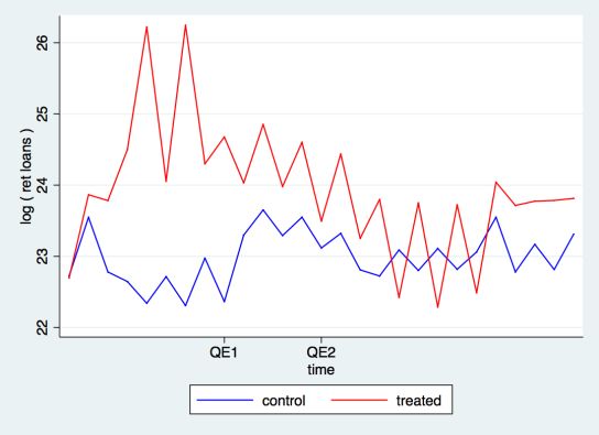
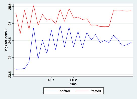
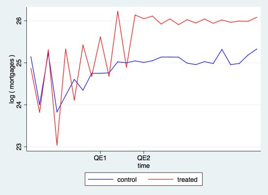
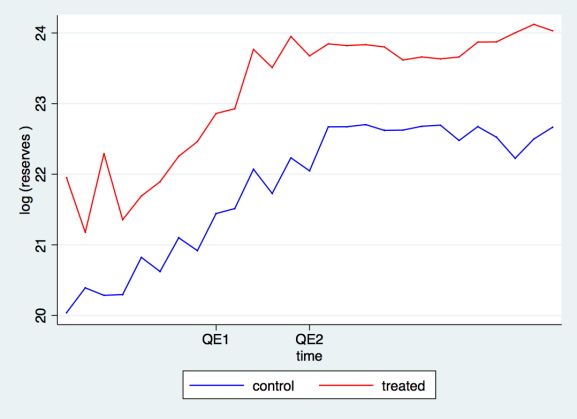
with replacement, i.e., matching ratio 1:5. Table 3 shows the effect of matching in eliminating average

differences between the two groups.7 The 2 test also confirms that we cannot reject the hypothesis

that all coefficients are equal to zero in the post-matching models as reported by the p value = 0.765.

For robustness checks, we vary the matching ratio between 1:1 and 1:8 reporting same results. The

 2 test reported in Table 9 of the Supplementary Materials confirms that we cannot reject the

hypothesis that all coefficients are zero in the post-matching models, suggesting that the 1:5 ratio is

the best compromise in terms of p-values and groups size.

5. Results

This section presents the difference-in-differences specifications and discusses three main sets of

findings. The first one investigates the impact of quantitative easing on the bank lending channel,

specifically on total lending, commercial and corporate lending, customer/retail lending and

mortgages. The second set of findings focuses on the asset allocation channel of QE-banks after the

implementation of the APP, specifically on lending to banks, reserves and government securities. The

third set of tests concentrates on the exposure of QE-banks to sovereign securities by employing a

sensitivity analysis of banks equity returns on returns on sovereigns. The last part of this section

discusses a list of robustness tests.

5.1. The Bank Lending Channel

We begin the analysis of the bank lending channel by showing the differences in lending behaviour

between treated and control groups as constructed in Section 4.2. Figure 3 plots the average group

trends reported in natural logs for total lending, corporate and commercial lending, customer/retail

lending and mortgages. In the pursuit of spotting interesting trends between the two groups that can

guide our empirical exercise, we can confirm that, in the pre QE1 phase, there is no clear evidence of

variation in the lending behaviour between the two groups, with the exception of customer/retail

loans.

7
 Note that some non-QE-banks have been matched with several treated banks more than once. We therefore retain the
 frequency weights from the matching for each non-discarded non-QE-bank as in Rodnyansky and Darmouni (2015).

 12

As we can see in Figure 3(c), treated banks started reducing their retail lending after QE1, with the

larger fall after QE2. According to Fatouh et al (2019), this fall can be driven by combination of lower

gilts yields (resulting from QE) and higher risk-based capital requirements, mainly affecting the

relatively larger QE banks. Control group banks, on the contrary, appear to have picked up the slack

by increasing their retail lending during the first wave of QE. In order to empirical validate the

evidences above, we estimate the following panel model

log( , ) = + + ( ) + , + ( , ) + , (1)

Figure 3 – Quantitative easing and the bank lending channel

(a) log of total lending (averaged by group) (b) log of commercial loans (averaged by group)

 (c) log of retail loans (averaged by group) (d) log of mortgages (averaged by group)

This figure plots the time series of the main bank lending channels as average values by the control and treated groups with
semi-annual frequency. Note that QE1 started in 2009h1 and QE2 in 2011h2. Panel (a) refers to the total lending series, (b)
to the corporate and commercial lending, (c) to the customer/retail lending and (4) to the mortgage lending. Absolute £
values are reported in logs.

where , is the log of total loans, corporate and commercial loans, customer/retail loans, or

mortgages, is a bank fixed effect, is an indicator variable that equals to 1 for the eight QE-

banks and 0 for the control group banks, = [ 1, , 2, ] is a set of two indicator variables that

 13

becomes one after the introduction of each QE wave. Specifically, the first wave QE1 started in 2009h1

while the second one QE2 started in 2011h28. The ∗ is the interaction term of the

treatment status and the QE episodes. The variable , is a matrix of controls that includes size

measured as the log of total assets, equity over total assets, return on assets (ROA) for profitability,

securities over total assets and net interest income over total assets to control for the business models

of the banks. As an alternative treatment status, we will also use a continuous treatment variable

 ( ℎ ) that equals to the log of the sum of reserves received by QE-banks and zero for non-

QE-banks. Following Rodnyansky and Darmouni (2015), we also include interaction terms , ∗ 

as robustness check for possible heterogeneous responses to the intervention by banks of different

nature. All standard errors are clustered at the bank level to allow for serial correlation across time.

We are interested in the element from equation (1) that represents the difference-in-differences

coefficient.

Table 4 reports the regression results of the log of total loans (1-2) and its decomposition into

corporate and commercial loans (3-4), customer/retail loans (5-6) and mortgages (7-8) using both

dummy and continuous treatment status. Confirming our initial impression from the average trends

of the two groups in Figure 3, we find no evidence that suggests QE directly boosted bank lending. We

note that after QE2, customer/retail loans of the treated banks were about 45% lower than the control

group, and the differences between QE1 and QE2 coefficients are different as reported by the p-value

at the bottom of Table 4. This suggests that QE2 reserves injections were associated with a decline in

lending at the macro level. Results are robust under the continuous treatment variable.

With a precise identification of the treated banks, we can confirm that the APP, which targeted gilts,

did not have a positive impact on the bank lending channel of QE-banks. The latter is an important

point to clarify. Although the lack of lending to the real economy at the macro level during the QE

8
 Butt et al. (2012) classify the QE expansion in July 2012 as a third wave. However, due to the short time gap with the last
 expansion of QE2 in February 2012, we did not differentiate them. This is also confirmed by an inequality test between
 coefficients of this QE3 and the other two that cannot reject the hypothesis that these coefficients are equal.

 14

periods is well established, this is not enough to rule out any possible bank lending channel as QE

reserves injections might have slowed down this decline in lending for QE-banks compared to non-

QE-banks. This result also finds supporting evidence in Rodnyansky and Darmouni (2015). They report

the failure of the second wave of the US asset purchase program, that specifically targeted Treasuries,

in boosting lending to the real economy, compared the other two that targeted instruments to which

banks were heavily exposed to, i.e., MSBs. This might raise the issue of the importance of the type of

asset being purchased in supporting the bank lending channel.

Table 4 – The Bank Lending Channel
 (1) (2) (3) (4) (5) (6) (7) (8)
 log(tot loans) log(comm loans) log(ret loans) log(mortgages)
 ∗ 1, 0.00132 -0.162 0.0263 0.0454
 (0.0642) (0.702) (0.331) (0.102)
 ∗ 2, 0.0954 0.192 -0.441** -0.0560
 (0.0959) (0.185) (0.160) (0.115)
 ( ℎ ) ∗ 1, -0.000165 -0.00714 8.51e-05 0.00199
 (0.00256) (0.0276) (0.0133) (0.00407)
 ( ℎ ) ∗ 2, 0.00424 0.00749 -0.0173** -0.00221
 (0.00379) (0.00738) (0.00638) (0.00458)

Observations 1,079 1,079 593 593 579 579 583 583
R-squared 0.595 0.595 0.502 0.502 0.532 0.532 0.708 0.708
Number of Banks 26 26 21 21 19 19 19 19
QE YES YES YES YES YES YES YES YES
Controls YES YES YES YES YES YES YES YES
Controls ∗ QE YES YES YES YES YES YES YES YES
Bank FEs YES YES YES YES YES YES YES YES
p-value 0.1288 0.1304 0.6968 0.6871 0.3979 0.4024 0.0201 0.0213

Coefficient estimates from specification of semiannual consolidated statements of UK banks from 2000h2 to 2018h1 using a
1:5 matching ratio. Treatment status equals to 1 for QE-banks and 0 for non-QE-banks. The continuous treatment
status ( ℎ ) equals to the log of the sum of reserves received by QE-banks and zero for non-QE-banks. Controls are
size as log of total assets, equity over total assets, return on assets (ROA), securities over total assets and net interest income
over total assets. The reported p-values test the coefficient inequality between QE1 and QE2. Standard errors are clustered
at the bank level and reported in brackets, * p

to the lower yields. This section looks deeper at corporate loans issuance by attempting a more direct

separation of credit supply from credit demand. As treatment and control banks are fundamentally

different, so are their borrowers. Therefore, we need to test the alternative explanation suggesting

that borrowers of QE banks demanded less credit over the post QE period. The test is performed by

employing the widely applied framework of Khwaja and Mian (2008) to identify credit demand effects

at the loan level.

Loan level data is retrieved from DealScan. We collect the total dollar amount of each loan for the

entire syndicate of lenders as well as the size of the loan of each separate lender using the loan shares

allocation. We manually matched 10 of our UK banks that were involved in syndicate loans, 5 of which

are QE banks. Khwaja and Mian (2008)’s framework defines the change in loan issuance for each bank-

firm pair before and after the treatment event as dependent variable. Following Rodnyansky and

Darmouni (2015) and Gropp et al. (2018), we selected a comparable time window that span between

two years before a QE event and two years after the event. The inclusion of firm fixed effects allows

us to control for any borrower characteristics that could have influenced the loan issuance. The model

estimated is the following:

 log(1 + , ) − log( , ) = + + , (2)

where , ( , ) is the total dollar value of the loan by lending bank i to borrowing firm j in the two

years after (before) the QE event, is the borrower firm fixed effect, is an indicator variable

that equals to 1 for the five QE-banks in the sample and 0 for the remaining banks, and , is the

idiosyncratic error term. All standard errors are double clustered at the bank and firm level.

Table 5 presents the estimation outputs for each of the two QE waves across several sets of controls,

including firm industry fixed effects in models (3-6) (using SIC1 digit as in Gropp et al., 2018), firm

country fixed effect in models (5-6) and the interaction of the two in (7-8) to absorb any endogenous

difference in borrower characteristics between the treatment and control group. In all specifications,

we find no evidence that lower lending by QE banks after the two QE waves is caused by differences

in the demand for loans between the treatment and control groups.

 16

Table 5 - Loan Issuance Estimator
 (1) (2) (3) (4) (5) (6) (7) (8)

 VARIABLES QE1 QE2 QE1 QE2 QE1 QE2 QE1 QE2

 0.0286 -0.204 0.112 -0.201 0.194 -0.271 0.399 0.0378
 (0.194) (0.183) (0.202) (0.181) (0.202) (0.211) (0.285) (0.173)

 Constant -0.0423 0.313 0.0915 0.381* -0.933*** 0.0688 -1.778*** 0.0837

 (0.208) (0.202) (0.224) (0.225) (0.346) (0.355) (0.298) (0.335)

 Observations 103 185 103 184 103 184 103 184

 R-squared 0.000 0.018 0.021 0.021 0.117 0.034 0.319 0.298

 Firm FE YES YES YES YES YES YES YES YES

 Industry FE YES YES YES YES

 Country FE YES YES

 Industry ∗ Country FE YES YES

Coefficient of the Khwaja and Mian (2008)’ estimates of the relative change in loan issuance by treated and control banks in
the two years before and after each the two QE waves. Treatment status equals to 1 for QE-banks and 0 for non-
QE-banks. The Industry fixed effect is evaluated using the SIC1 code. Standard errors are double clustered at the bank and
firm level and reported in brackets, * p

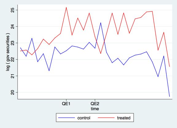
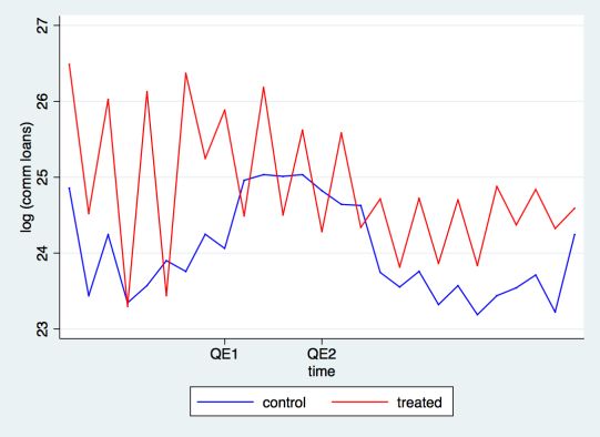
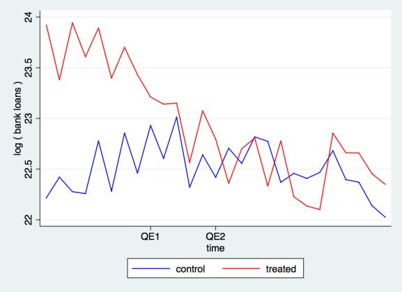
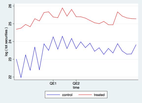
Figure 4 – Quantitative easing and the asset reallocation channel

 (a) log of reserves (averaged by group) (b) log of bank loans (averaged by group)

 (c) log of total securities (averaged by group) (d) log of government securities (averaged by group)

This figure plots the time series of the main asset reallocation channels as average values by the control and treated groups
with semi-annual frequency. Note that QE1 started in 2009h1 and QE2 in 2011h2. Panel (a) refers to the reserves series, (b)
to the lending to banks, (c) to total securities and (4) to government securities. Absolute £ values are in logs.

The positive gap in reserves might infer that treated banks took advantage of the QE cash to restore

and/or increase their liquidity. However, when looking at the other assets we clearly observe a

reduction of interbank lending (Panel b) by the treated banks as well as an increase of government

securities as plotted on Figure 4 (b) and (d) respectively. This could indicate that treated banks might

have reallocated their assets from high risk-weighted instruments (like retail loans and bank loans)

towards other assets with lower risk weights like government securities. This is also in line with the

fact that this difference disappears when looking at the total securities trends of Figure 4 (c). We also

note that there is a big fall in 2012 of the treated banks’ exposure to government securities right at

the peak of the EU sovereign debt crisis, in line with what is reported by Acharya and Steffen (2015)

on the unwinding of the carry trade strategy by European banks.

 18

This evidence motivated our next set of empirical tests aimed at assessing the impact of QE on the log

 of reserves, bank loans, total securities and government securities.

 Table 6 – The Asset Reallocation Effect
 (1) (2) (3) (4) (5) (6) (7) (8)
 log(deposits) log(reserves) log(bank loans) log(gov securities)
 ∗ 1, 0.0700 0.594* -0.877*** 0.418*
 (0.0743) (0.306) (0.272) (0.209)
 ∗ 2, 0.0588 -0.371 -0.348 0.541***
 (0.0993) (0.233) (0.272) (0.174)
 ( ℎ ) ∗ 1, 0.00262 0.0245* -0.0356*** 0.0167*
 (0.00305) (0.0126) (0.0112) (0.00817)
 ( ℎ ) ∗ 2, 0.00292 -0.0142 -0.0135 0.0215***
 (0.00382) (0.00946) (0.0112) (0.00680)

Observations 1,057 1,057 1,078 1,078 1,062 1,062 650 650
R-squared 0.364 0.364 0.643 0.643 0.180 0.179 0.415 0.415
Number of Banks 25 25 27 27 25 25 24 24
QE YES YES YES YES YES YES YES YES
Controls YES YES YES YES YES YES YES YES
Controls ∗ QE YES YES YES YES YES YES YES YES
Bank FEs YES YES YES YES YES YES YES YES
p-value 0.0055 0.0059 0.8199 0.7958 0.6066 0.5978 0.6046 0.6134

 Coefficient estimates from specification of semiannual consolidated statements of UK banks from 2000h2 to 2018h1 using a
 1:5 matching ratio. Treatment status equals to 1 for QE-banks and 0 for non-QE-banks. The continuous treatment
 status ( ℎ ) equals to the log of the sum of reserves received by QE-banks and zero for non-QE-banks. Controls are
 size as log of total assets, equity over total assets, return on assets (ROA), securities over total assets and net interest income
 over total assets. The reported p-values test the coefficient inequality between QE1 and QE2. Standard errors are clustered
 at the bank level and reported in brackets, * p

The carry trade activity by European banks towards zero-to-low risk-weighted sovereign debt

provided higher returns during this period at no (or little) extra cost of capital. Our results suggest that

QE has facilitated this bank behavior. We confirm this in Section 5.5 by testing the sensitivity of UK

treated banks equity returns on GIIPS and German bond returns in the same vein as Acharya and

Steffen (2015).

5.4. The Timing of Effects

Rodnyansky and Darmouni (2015) suggest a supplementary robustness test on the timing of effects

to confirm that our asset reallocation effects actually happened after the QE waves. We follow their

model specification by estimating a fixed-effect regression using the matched sample of banks as

follows

log( , ) = + ∑ + ∑ ( ) + , + ∑ ( , ) + , (3)

where , is the log of customer/retail lending, reserves, bank loans and government securities9, is

a bank fixed effect, is an indicator variable that equals 1 for the eight QE-banks and 0 for

the control group banks, is an indicator function of the time period (semi-annual) from 2007h1 to

2018h1 with 2006h2 as the omitted category. × is the interaction term of the treatment

status and the time dummies. , is a matrix of controls that includes size measured as the log of total

assets, equity over total assets, return on assets (ROA) for profitability, securities over total assets and

net interest income over total assets. In line with equation (1), we also include interaction terms , ×

 as robustness check.

Figure 5 validates our findings by confirming the timing of the main effects. Starting from panel (a), a

steady decline after QE2 is observed for customer/retail loans. The trend of reserves in panel (b)

appears to start its climb in the first half of 2010 reaching a peak in 2011h1, after the start of QE1. This

trend looks more stable after QE2 and is in line with our findings. We find that same results but

opposite sign for the loans to banks in panel (c) that show a clear decline from 2009h2 till 2010h2.

9 We also tested the other dependent variables used in our exercises that show no significant impact. Figures are reported
 in the Supplementary Materials Error! Reference source not found..

 20

This trend then stabilises in the QE2 period. Finally, panel (c) report the time coefficients for the

government securities model. Although we notice some volatility, we observe the positive trend after

each of the QE waves, noting that the big fall of 2012h2 is very likely to have been caused by the EU

sovereign debt crisis that forced those banks involved in carry trade activity to unwind their positions

(Acharya and Steffen, 2015).

Figure 5 – Time coefficients
35 3
 QE1 QE2 QE1 QE2
 2.5
30

 2
25
 1.5

20 1

 0.5
15
 0

10 -0.5

 -1
 5

 -1.5
 0
 -2

-5 -2.5
 20 1

 20 2

 20 1

 20 2

 20 1

 20 2

 20 1

 20 2

 20 1

 20 2

 20 1

 20 2

 20 1

 20 2

 20 1

 20 2

 20 1

 20 2

 20 1

 20 2

 20 1

 20 2
 h1

 20 1

 20 2

 20 1

 20 2

 20 1

 20 2

 20 1

 20 2

 20 1

 20 2

 20 1

 20 2

 20 1

 20 2

 20 1

 20 2

 20 1

 20 2

 20 1

 20 2

 20 1

 20 2
 h1
 h

 h

 h

 h

 h

 h

 h

 h

 h

 h

 h

 h

 h

 h

 h

 h

 h

 h

 h

 h

 h

 h

 h

 h

 h

 h

 h

 h

 h

 h

 h

 h

 h

 h

 h

 h

 h

 h

 h

 h

 h

 h

 h

 h
 07

 07

 08

 08

 09

 09

 10

 10

 11

 11

 12

 12

 13

 13

 14

 14

 15

 15

 16

 16

 17

 17

 18

 07

 07

 08

 08

 09

 09

 10

 10

 11

 11

 12

 12

 13

 13

 14

 14

 15

 15

 16

 16

 17

 17

 18
 20

 20

 (a) log of retail loans (b) log of reserves
 1.5
 15
 QE1 QE2 QE1 QE2
 1

 0.5 10

 0

 5
-0.5

 -1
 0
-1.5

 -2
 -5
-2.5

 -3
 -10

-3.5

 -4 -15
 20 1

 20 2

 20 1

 20 2

 20 1

 20 2

 20 1

 20 2

 20 1

 20 2

 20 1

 20 2

 20 1

 20 2

 20 1

 20 2

 20 1

 20 2

 20 1

 20 2

 20 1

 20 2
 h1

 20 1

 20 2

 20 1

 20 2

 20 1

 20 2

 20 1

 20 2

 20 1

 20 2

 20 1

 20 2

 20 1

 20 2

 20 1

 20 2

 20 1

 20 2

 20 1

 20 2

 20 1

 20 2
 h1
 h

 h

 h

 h

 h

 h

 h

 h

 h

 h

 h

 h

 h

 h

 h

 h

 h

 h

 h

 h

 h

 h

 h

 h

 h

 h

 h

 h

 h

 h

 h

 h

 h

 h

 h

 h

 h

 h

 h

 h

 h

 h

 h

 h
 07

 07

 08

 08

 09

 09

 10

 10

 11

 11

 12

 12

 13

 13

 14

 14

 15

 15

 16

 16

 17

 17

 18
 07

 07

 08

 08

 09

 09

 10

 10

 11

 11

 12

 12

 13

 13

 14

 14

 15

 15

 16

 16

 17

 17

 18

 20
 20

 (a) log of loans to banks (b) log of government securities

This figure plots the coefficients of equation (2) with the 95% confidence intervals for each semiannual time dummy from
2007h1 to 2018h1 with 2006h2 as the omitted category. Dashed lines mark the beginning of the two QE waves.

Note that the variable ‘government securities’ might not fully capture the asset reallocation channel

of banks towards sovereign securities (mainly from GIIPS countries) as this balance sheet variable does

not distinguish between securities and their risk weighting. Section 5.5 provides additional empirical

evidence of the exposure of QE banks to specific sovereigns to support this claim.

5.5. Exposure to Sovereigns

This section investigates the exposure of treated banks to sovereigns during the two QE periods by

using market data. Due to the lack of micro-level data of sovereign positions, we employ Acharya and

 21

Steffen (2015)’s sensitivity analysis of banks’ stock returns to returns on sovereigns, estimating the

following model

 , = + , + , + ( , ) +

 ( , ) + + , (4)

where , is the daily stock return of UK bank i, is a bank fixed effect, is an indicator

variable that equals to 1 for the QE-banks and 0 for the control group banks, , is the daily

return of ten-year government bonds from Greece, Italy, Ireland, Portugal or Spain (GIIPS). We also

include government bond returns of UK, Germany, US and Japan. , is the FTSE 350 daily

return orthogonalized by both UK and German bond return series10, and is the vector of

macroeconomic state controls variables.11 According to the authors, a combination of positive

loadings of the coefficients for the GIIPS countries combined with a negative loading for that of

Germany is consistent with carry trade behaviour by banks. By controlling for the treated banks, the

estimation of our difference-in-differences coefficients can shed a light on the role of QE in

promoting the carry trade in Europe and therefore confirming our asset reallocation channel

hypothesis. More precisely, if QE banks reallocated APP reserves injections towards peripheral EU

countries sovereigns, we would expect positive loads on some of the GIIPS countries’ coefficients as

well as a negative load for German bonds.

Equation (4) is estimated using pooled ordinary least squares regressions with standard error

clustered at both bank and time level. The control group is reconstructed among listed non-QE banks

following the same propensity score matching procedure and list of covariates reported in Section 4.2

for consistency. The results are reported in Table 7.

10 Following Acharya and Steffen (2015), we use the residual from the regression of the FTSE daily log returns on daily UK
 Gilts and German bund returns. As robustness we also replaced FTSE 350 with the FTSE 100 index (not reported) with no
 changes in the results.
11 We include all the control variables from Acharya and Steffen (2015) model: “VSTOXX, the change in the volatility index of

 the European stock market; TermStructure, measured as the difference between the yield on a 10-year euro area
 government bond and the one-month Euribor; BondDefSpread, the difference between the yield on 10-year German BBB
 bonds and yields on 10-year German government debt; 1mEuribor, the one-month Euribor; ΔESI, the monthly change in
 the economic sentiment indicator; ΔIntProd, the monthly change in the level of industrial production; ΔCPI, the change in
 the rate of inflation measured as the monthly change in the European consumer price index; and ΔFX-Rate, the change in
 the effective exchange rate of the euro” (pg. 221, footnote 20).

 22

Table 7 - Banks's sensitivity to Sovereign Exposures on Individual GIIPS
 Panel A - DiD on QE1
 (1) (2) (3) (4) (5)
 VARIABLES GRE ITA IRI POR SPA

 0.0103
 (0.00805)
 ∗ 0.00962
 (0.0138)
 0.0570**
 (0.0272)
 ∗ 0.170***
 (0.0423)
 0.0383
 (0.0321)
 ∗ 0.107**
 (0.0526)
 0.0273
 (0.0213)
 ∗ 0.0733**
 (0.0328)
 0.0552*
 (0.0319)
 ∗ 0.138***
 (0.0505)
 -0.547*** -0.547*** -0.546*** -0.546*** -0.549***
 (0.0619) (0.0618) (0.0618) (0.0618) (0.0619)
 ∗ -0.105 -0.101 -0.104 -0.102 -0.108
 (0.0942) (0.0940) (0.0941) (0.0941) (0.0941)
 -1.032*** -1.051*** -1.053*** -1.043*** -1.050***
 (0.0778) (0.0772) (0.0790) (0.0775) (0.0772)
 ∗ -0.369*** -0.396*** -0.410*** -0.380*** -0.397***
 (0.114) (0.114) (0.117) (0.114) (0.114)
 -0.0471 -0.0445 -0.0444 -0.0469 -0.0459
 (0.0491) (0.0491) (0.0492) (0.0491) (0.0491)
 ∗ -0.0533 -0.0613 -0.0551 -0.0584 -0.0619
 (0.0785) (0.0785) (0.0786) (0.0786) (0.0785)
 -0.194** -0.169* -0.180* -0.185** -0.170*
 (0.0939) (0.0950) (0.0943) (0.0943) (0.0947)
 ∗ 0.515*** 0.387*** 0.460*** 0.465*** 0.427***
 (0.0853) (0.0911) (0.0882) (0.0872) (0.0923)
 1.065*** 1.065*** 1.067*** 1.066*** 1.065***
 (0.0288) (0.0290) (0.0288) (0.0287) (0.0290)
 ∗ 0.136*** 0.113*** 0.129*** 0.127*** 0.122***
 (0.0336) (0.0342) (0.0336) (0.0336) (0.0343)

 Observations 49,604 49,604 49,604 49,604 49,604
 R-squared 0.372 0.373 0.372 0.372 0.373
 Macro Controls YES YES YES YES YES
 Bank FEs YES YES YES YES YES

 23

Panel B - DiD on QE2
 (1) (2) (3) (4) (5)
 VARIABLES GRE ITA IRI POR SPA

 0.00988
 (0.00716)
 ∗ 0.00171
 (0.0113)
 0.0628**
 (0.0290)
 ∗ 0.169***
 (0.0432)
 0.115**
 (0.0564)
 ∗ 0.0201
 (0.0884)
 0.0512**
 (0.0253)
 ∗ 0.0484
 (0.0357)
 0.0764**
 (0.0367)
 ∗ 0.129**
 (0.0561)
 -0.585*** -0.583*** -0.583*** -0.581*** -0.587***
 (0.0694) (0.0692) (0.0691) (0.0689) (0.0694)
 ∗ -0.0452 -0.0330 -0.0446 -0.0398 -0.0443
 (0.0998) (0.0989) (0.0992) (0.0990) (0.0993)
 -1.013*** -1.034*** -1.074*** -1.028*** -1.034***
 (0.0831) (0.0819) (0.0865) (0.0824) (0.0819)
 ∗ -0.325*** -0.349*** -0.336*** -0.334*** -0.348***
 (0.109) (0.108) (0.115) (0.108) (0.108)
 -0.0824 -0.0776 -0.0799 -0.0834 -0.0803
 (0.0560) (0.0559) (0.0560) (0.0560) (0.0560)
 ∗ -0.0881 -0.0892 -0.0883 -0.0909 -0.0938
 (0.0803) (0.0803) (0.0803) (0.0804) (0.0802)
 -0.211* -0.184 -0.211* -0.205* -0.180
 (0.115) (0.117) (0.117) (0.116) (0.116)
 ∗ 0.453*** 0.299*** 0.446*** 0.413*** 0.354***
 (0.0896) (0.0937) (0.0948) (0.0902) (0.0954)
 1.105*** 1.101*** 1.099*** 1.099*** 1.099***
 (0.0333) (0.0335) (0.0332) (0.0330) (0.0337)
 ∗ 0.0104 -0.0240 0.00940 0.00145 -0.0107
 (0.0358) (0.0361) (0.0358) (0.0357) (0.0365)

 Observations 49,604 49,604 49,604 49,604 49,604
 R-squared 0.364 0.365 0.365 0.365 0.365
 Macro Controls YES YES YES YES YES
 Bank FEs YES YES YES YES YES
Coefficient estimates from specification of daily equity returns of UK banks using a 1:4 matching ratio. Treatment
status equals to 1 for QE-banks and 0 for non-QE-banks. Panel A reports estimates from the period of QE1 (5th of
March 2009) onwards whereas Panel B considers the QE2 period only (6th of October 2011 onwards). Variables GR, IT, IR,
PR, SP, UK, GE and JP are daily returns of 10 years bond of Greece, Italy, Ireland, Portugal, Spain, UK, Germany and Japan
respectively. Macro Controls are (i) VSTOXX, the change in the volatility index of the European stock market; (ii)
TermStructure, measured as the difference between the yield on a 10-year euro area government bond and the one-month
Euribor; (iii) BondDefSpread, the difference between the yield on 10-year German BBB bonds and yields on 10-year German
government debt; (iv) 1mEuribor, the one-month Euribor; (v) ΔESI, the monthly change in the economic sentiment indicator;
(vi) ΔIntProd, the monthly change in the level of industrial production; (vii) ΔCPI, the change in the rate of inflation measured
as the monthly change in the European consumer price index; and (viii) ΔFX-Rate, the change in the effective exchange rate
of the euro. Standard errors are double clustered at the bank and time level and reported in brackets, * p

Panel A in Table 7 reports estimates from the period of QE1 (5th of March 2009) onwards whereas

Panel B considers the QE2 period only (6th of October 2011 onwards). Due to the high correlation of

the GIIPS bond returns, we test the sensitivity of equity returns of UK banks with GIIPS bond returns

individually. However, we also report models when controlling for all GIIPS returns in Supplementary

Table 14 for robustness.

When controlling for the impact of QE via the asset reallocation channel, we find that this exposure

was larger for QE banks. In QE1, positive factor loadings of all GIIPS diff-in-diff interaction terms 

except for Greek bonds, along with negative loading of (the interaction term of German

bonds and treated status) in Table 7 confirm our previous findings that QE banks reinvested APP

reserves injections into low-to-zero risk weighted GIIPS sovereigns. Note that the insignificant

coefficient of Greek bonds can be easily explained by the lack of confidence in the country which was

facing sovereign debt crisis problems over the period in question.

During QE2, this effect is mainly concentrated on Italian and Spanish bonds. Note that those were

most popular sovereigns used by European banks as part of the carry trade activity (Acharya and

Steffen, 2015). We also note the positive loadings of for treated banks. This can be puzzling,

given the very low yields on Japanese government bonds. However, we believe QE banks might have

channelled a part of APP reserves into these bonds, anticipating a boost in their prices when the Bank

of Japan (BOJ) relaunch its QE program, following its announcement in October 2010 that it would

examine the purchase of ¥5 trillion of assets. BOJ implemented this a year later in October 2011. Since

this is very close to the start of UK QE2, we can validate our proposition about the stockpiling of

Japanese government bonds by QE banks by comparing the coefficients of Japanese government

bonds in QE1 and QE2. Indeed, Supplementary Table 18 shows the coefficient of Japanese government

bonds is significant in QE1 and insignificant in QE2.

We also test the baseline models of Acharya and Steffen (2015) for UK banks in Supplementary Table

14 (models 1 and 3) with the diff-in-diff models (2) and (4). Estimates of Model (1) are well matched

with both signs and magnitudes of factor loadings of Acharya and Steffen (2015)’s findings. We report

 25