Predicting Gold and Silver Price Direction Using Tree-Based Classifiers - MDPI
←
→
Page content transcription
If your browser does not render page correctly, please read the page content below
Journal of
               Risk and Financial
               Management

Article
Predicting Gold and Silver Price Direction Using
Tree-Based Classifiers
Perry Sadorsky

                                          Schulich School of Business, York University, Toronto, ON M3J 1P3, Canada; psadorsky@schulich.yorku.ca

                                          Abstract: Gold is often used by investors as a hedge against inflation or adverse economic times.
                                          Consequently, it is important for investors to have accurate forecasts of gold prices. This paper
                                          uses several machine learning tree-based classifiers (bagging, stochastic gradient boosting, random
                                          forests) to predict the price direction of gold and silver exchange traded funds. Decision tree bagging,
                                          stochastic gradient boosting, and random forests predictions of gold and silver price direction are
                                          much more accurate than those obtained from logit models. For a 20-day forecast horizon, tree
                                          bagging, stochastic gradient boosting, and random forests produce accuracy rates of between 85%
                                          and 90% while logit models produce accuracy rates of between 55% and 60%. Stochastic gradient
                                          boosting accuracy is a few percentage points less than that of random forests for forecast horizons
                                          over 10 days. For those looking to forecast the direction of gold and silver prices, tree bagging and
                                          random forests offer an attractive combination of accuracy and ease of estimation. For each of gold
                                          and silver, a portfolio based on the random forests price direction forecasts outperformed a buy and
                                          hold portfolio.

                                Keywords: gold and silver prices; forecasting; machine learning; random forests; bagging; stochastic

                                          gradient boosting
Citation: Sadorsky, Perry. 2021.
Predicting Gold and Silver Price
Direction Using Tree-Based
Classifiers. Journal of Risk and
                                          1. Introduction
Financial Management 14: 198.
https://doi.org/10.3390/jrfm                    A principal concern for investors in financial assets is how to protect their investment
14050198                                  portfolios from adverse movements in the market. Gold is often used by investors as
                                          a hedge against inflation or adverse economic times (Baur and Lucey 2010; Baur and
Academic Editor: Jong-Min Kim             McDermott 2010; Bekiros et al. 2017; Ciner et al. 2013; Hood and Malik 2013; Junttila et al.
                                          2018; Baur and McDermott 2016; Beckmann et al. 2015; Blose 2010; Hoang et al. 2016;
Received: 13 April 2021                   Reboredo 2013; Iqbal 2017; O’Connor et al. 2015; Hillier et al. 2006; Tronzano 2021; Areal
Accepted: 27 April 2021                   et al. 2015). For example, gold prices increased during the 2008–2009 global financial crisis
Published: 29 April 2021                  (GFC) and during the COVID19 pandemic. In response to the COVID19 pandemic, London
                                          morning gold prices increased 35% from USD 1523 on 31 December 2019 to USD 2049 on 6
Publisher’s Note: MDPI stays neutral      August 2020 (ICE Benchmark Administration Limited (IBA) 2021).
with regard to jurisdictional claims in         Given the interest in gold as an asset it is not surprising that there are many studies
published maps and institutional affil-
                                          that forecast the price of gold. Examples of methods used to forecast gold prices include
iations.
                                          econometrics (Shafiee and Topal 2010; Aye et al. 2015; Hassani et al. 2015; Gangopadhyay
                                          et al. 2016), artificial neural networks (Kristjanpoller and Minutolo 2015; Alameer et al.
                                          2019; Parisi et al. 2008), boosting (Pierdzioch et al. 2015, 2016a, 2016b), random forests (Liu
                                          and Li 2017; Pierdzioch and Risse 2020), support vector machines (Risse 2019), and other
Copyright: © 2021 by the author.          machine learning methods (Yazdani-Chamzini et al. 2012; Livieris et al. 2020; Mahato and
Licensee MDPI, Basel, Switzerland.        Attar 2014).
This article is an open access article          Looking first at some representative research that uses traditional econometric meth-
distributed under the terms and
                                          ods to predict gold prices, Shafiee and Topal (2010) propose a time series model for monthly
conditions of the Creative Commons
                                          gold prices that consists of a long-term reversion component, a diffusion component, and a
Attribution (CC BY) license (https://
                                          jump component. In a forecasting comparison, this model has lower root mean squared
creativecommons.org/licenses/by/
                                          error (RMSE) than an ARIMA model. Aye et al. (2015) use dynamic model averaging,
4.0/).

J. Risk Financial Manag. 2021, 14, 198. https://doi.org/10.3390/jrfm14050198                                   https://www.mdpi.com/journal/jrfm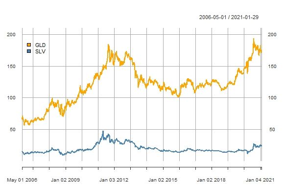
J. Risk Financial Manag. 2021, 14, 198                                                                                          2 of 21

                                         dynamic model selection and Bayesian model averaging to forecast monthly gold prices.
                                         They find that these models outperform a random walk. They use financial variables and
                                         real economic variables as explanatory variables and find that financial variables have
                                         stronger predictive power. Using time series techniques (vector autoregression, ARIMA,
                                         ETS, TBATS) to forecast monthly gold price Hassani et al. (2015) find, however, that it
                                         is difficult to beat a random walk. In a forecasting comparison of Indian gold prices,
                                         Gangopadhyay et al. (2016) find that a vector error correction model outperforms a ran-
                                         dom walk.
                                               Representative research that uses machine learning (ML) methods to predict gold
                                         prices includes the following. Parisi et al. (2008) use artificial neural networks (ANN)
                                         to forecast the change in weekly gold prices. Lagged gold price changes and lagged
                                         changes in the Dow Jones Index are used as explanatory variables. They find that rolling
                                         ward networks have better forecasting accuracy than either recursive ward networks or
                                         feed forward networks. Yazdani-Chamzini et al. (2012) compare the monthly gold price
                                         forecasting performance of ANN, adaptive neuro-fuzzy inference system (ANFIS), and
                                         ARIMA. They find that ANFIS outperforms the other models and the results are robust to
                                         different training and test sets. Mahato and Attar (2014) predict gold prices using ensemble
                                         methods. Using stacking and hybrid bagging they find gold and silver price accuracy of
                                         85% and 79%, respectively. Kristjanpoller and Minutolo (2015) use ANN-GARCH models
                                         to forecast daily gold price volatility. They find that the ANN-GARCH model results in
                                         a 25% reduction in mean average prediction error over the GARCH model. Pierdzioch
                                         et al. (2015) use regression boosting to forecast monthly gold prices. They find that the
                                         explanatory variables (inflation rates, exchange rates, stock market, interest rates) have
                                         predictive power, but the trading rules generated do not beat a simple buy and hold
                                         strategy. Pierdzioch et al. (2016a) use quantile regression boosting to forecast gold prices.
                                         Trading rules generated from this approach can, in some situations (low trading costs,
                                         and specific quantiles) beat that of a buy and hold strategy. Pierdzioch et al. (2016b) use
                                         a boosting regression to forecast gold price volatility. Boosting provides better forecasts
                                         compared to an autoregressive model. Alameer et al. (2019) use monthly data to forecast the
                                         price of gold using a neural network with a whale optimization algorithm. This approach
                                         has better forecasting performance compared to several other machine learning methods
                                         (classic neural network, particle swarm neural network, and grey wolf optimization)
                                         and ARIMA models. Risse (2019) takes a novel approach and combines wavelets and
                                         support vector machine (SVM) to predict monthly gold prices. The feature space includes
                                         variables for interest rates, exchange rates, commodity prices, and stock prices. Wavelets
                                         are applied to each of these predictors in order to generate additional features for the
                                         SVM. The wavelet SVM produces more accurate gold price forecasts than other models
                                         like SVM, random forest, or boosting. Livieris et al. (2020) combine deep learning with
                                         long short-term memory (LSTM) to predict gold prices. The addition of the LSTM layers
                                         to the deep learning process provides an increase in forecasting performance. Pierdzioch
                                         and Risse (2020) use random forests to predict the returns of gold, silver, platinum, and
                                         palladium. They find that forecasts from multivariate models are more accurate than
                                         forecasts from univariate models. Plakandaras et al. (2021) combine ensemble empirical
                                         mode decomposition with SVM to predict monthly gold prices. The feature set contains
                                         interest rates and asset price variables. They use a two-step process where in the first
                                         step the data are filtered and then in the second step the filtered data are used in a SVM.
                                         Forecast accuracy is higher than that obtained from ordinary least squares or least absolute
                                         shrinkage. This literature described above shows that machine learning methods appear to
                                         offer better gold price forecasting accuracy than traditional econometric methods.
                                               The use of ML methods to evaluate investment trading strategies is becoming more
                                         widely adopted. Here, are a few representative examples. Jiang et al. (2020) use extreme
                                         gradient boosting to predict stock prices and combine this with a risk adjusted portfolio
                                         rebalancing. They find that their approach provides better risk adjusted returns relative
                                         to a buy and hold strategy. Kim et al. (2019) use hidden Markov models to devise global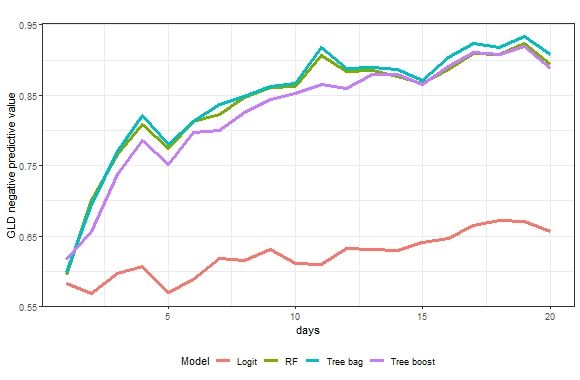
J. Risk Financial Manag. 2021, 14, 198                                                                                            3 of 21

                                         asset allocation strategies. They find that the hidden Markov model produces trading
                                         strategies that outperform (in terms of risk and return measure) traditional momentum
                                         strategies. Koker and Koutmos (2020) use reinforcement learning techniques to devise
                                         trading strategies for five cryptocurrencies. Compared to a buy and hold strategy this
                                         approach yields better risk adjusted returns. Suimon et al. (2020) use the autoencoder
                                         ML approach to investigate a long and short trading strategy for Japanese government
                                         bonds. This approach has better investment performance than a trend following strategy.
                                         Vezeris et al. (2019) develop an improved Turtle trading system that they call AdTurtle
                                         which outperforms the classic Turtle trading system. Zengeler and Handmann (2020)
                                         use recurrent long short term memory networks to trade contracts for difference. Their
                                         approach outperforms the market.
                                               The purpose of this paper is to predict gold and silver price direction using tree-based
                                         classifiers. This paper differs from the existing literature in six important ways. First,
                                         there is research showing that predicting stock price direction is more successful than
                                         predicting actual stock prices (Basak et al. 2019; Leung et al. 2000; Nyberg 2011; Nyberg and
                                         Pönkä 2016; Pönkä 2016; Ballings et al. 2015; Lohrmann and Luukka 2019; Sadorsky 2021).
                                         Unlike much of the existing literature on gold price forecasting that focusses on gold prices,
                                         this paper predicts gold price direction. Second, much of the existing literature on gold
                                         price forecasting uses macroeconomic variables for features. In the stock price forecasting
                                         literature, there is evidence that technical indicators are useful for predicting stock prices
                                         (Yin and Yang 2016; Yin et al. 2017; Neely et al. 2014; Wang et al. 2020; Bustos and Pomares-
                                         Quimbaya 2020). This paper uses technical indicators as features for predicting gold price
                                         direction. Feature selection is based on several well-known technical indicators like moving
                                         average, stochastic oscillator, rate of price change, MACD, RSI, and advance decline line
                                         (Bustos and Pomares-Quimbaya 2020). Third, this paper predicts gold and silver price
                                         direction using tree-based classifiers like random forests (RFs), bagging, and stochastic
                                         gradient boosting. Bagging, tree boosting, and RFs are based on the concept of a decision
                                         tree (James et al. 2013; Hastie et al. 2009) and often provide a good balance between ease
                                         of estimation and accuracy. While there is research on using these methods to predict
                                         gold prices, there is little known about how useful these methods are for forecasting gold
                                         price direction. Fourth, gold and silver prices are measured using exchange traded funds
                                         (ETFs). ETFs are convenient for investors who want to participate in commodity markets
                                         but do not want to deal with the intricacies of owning a futures account. Fifth, directional
                                         stock price forecasts are constructed from one day to twenty days in the future. A five
                                         day forecast horizon corresponds to one week of trading days, a 10 day forecast horizon
                                         corresponds to two weeks of trading days and a twenty day forecast horizon corresponds
                                         to approximately one month of trading days. Forecasting stock price direction over a
                                         multi-day horizon provides more information on how prediction accuracy changes across
                                         the forecast period. Sixth, the practical significance of these results is further investigated
                                         using a portfolio investment comparison.
                                               The analysis from this research provides some interesting results. At all forecast hori-
                                         zons, RFs and tree bagging show much better gold and silver ETF price prediction accuracy
                                         then logit. The prediction accuracy from bagging and RFs is very similar indicating that
                                         either method is very useful for predicting the price direction of gold and silver ETFs. The
                                         prediction accuracy for RF and tree bagging models is over 85% for forecast horizons of 10
                                         days or more. Stochastic gradient boosting accuracy is a few percentage points less than
                                         that of random forests for forecast horizons over 10 days. For a 20-day forecast horizon, tree
                                         bagging, stochastic gradient boosting, and random forests have accuracy rates of between
                                         85% and 90% while logit models have accuracy rates of between 55% and 60%. For each
                                         of gold and silver, an investment portfolio based on the random forests price direction
                                         forecasts outperforms a buy and hold portfolio.
                                               This paper is organized as follows. The next section sets out the methods and data.
                                         This is followed by the results. The last section of the paper provides some conclusions
                                         and suggestions for future research.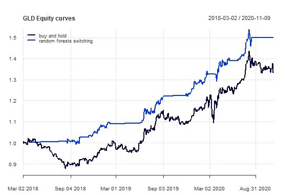
J. Risk Financial Manag. 2021, 14, 198                                                                                                    4 of 21

                                         2. Methods and Data
                                         2.1. The Logit Method for Prediction
                                              The direction of stock price changes can be classified as either up (stock price change
                                         from one period to the next is positive) or down (stock price change from one period to
                                         the next is non-positive). A standard classification problem like this where the variable
                                         of interest can take on only one of two values (up or down) is easily coded as a binary
                                         variable. Logit models are one widely used approach to modelling and forecasting binary
                                         variables and logit models can be used to predict the direction of stock prices. Explanatory
                                         variables considered pertinent to predicting stock price direction can be used as features.
                                         Logit models are easy to estimate and widely used to predict binary classification outcomes
                                         (James et al. 2013).
                                                                             yt+h = α + βXt + εt ,                                 (1)
                                               In Equation (1), yt+h = pt+h – pt is a binary variable that takes on the value of “up” if
                                         positive or “down” if non-positive and X is a vector of features. The variable pt represents
                                         the adjusted closing stock price on day t. The random error term is ε. The symbol h denotes
                                         the forecast horizon, h = 1, 2, 3, . . . , 20, and indicates the number of time periods into
                                         the future to predict. A multistep forecast horizon is used in order to see how forecast
                                         accuracy changes across the forecast horizon. A 5-day forecast corresponds to one week
                                         of trading data, a 10 day forecast corresponds to two weeks of trading data, and a 20 day
                                         forecast is consistent with the average number of trading days in a month. The features
                                         used in the analysis include familiar technical indicators like the relative strength indicator
                                         (RSI), stochastic oscillator (slow, fast), advance–decline line (ADX), moving average cross-
                                         over divergence (MACD), price rate of change (ROC), on balance volume (OBV), the
                                         50-day moving average, 200-day moving average, money flow index (MFI), and Williams
                                         accumulation and distribution (WAD). The technical indicators used in this paper are
                                         widely used in academics and practice (Yin and Yang 2016; Yin et al. 2017; Neely et al. 2014;
                                         Wang et al. 2020; Bustos and Pomares-Quimbaya 2020). Achelis (2013) provides a detailed
                                         description of the calculation of these technical indicators.

                                         2.2. Decision Trees and Bagging for Prediction
                                               Logit regression classifies the dependent (response) variable using a linear bound-
                                         ary and this can be restrictive in circumstances where there is a nonlinear relationship
                                         between the response and the features. Decision trees are better able to capture the clas-
                                         sification between the response and the features in nonlinear situations by bisecting the
                                         predictor space into smaller and smaller non-overlapping regions. The rules used to split
                                         the predictor space can be summarized in a tree diagram, and this approach is known
                                         as a decision tree method. Tree-based methods are easy to interpret but are not as com-
                                         petitive with other methods like bagging, boosting or random forests. The main ideas
                                         behind decision trees, bagging, boosting, and random forest methods is presented in the
                                         following paragraphs and a more complete treatment of these topics can be found in
                                         James et al. (2013) and Hastie et al. (2009).
                                               A qualitative response can be predicted using a classification tree. A classification
                                         tree predicts that each observation belongs to the most commonly occurring class of
                                         training observations in the region to which it belongs. A majority voting rule is used for
                                         classification. The basic steps in building a classification tree can be described as follows.
                                               1. The predictor space (for all possible values of X1 , . . . , XP ) is divided into J distinctive
                                         and non-overlapping regions, R1 , . . . , RJ .
                                               2. For every observation that falls into the region Rj, the same prediction is made.
                                         This prediction is that each observation belongs to the most commonly occurring class of
                                         training observations to which it belongs.
                                               The construction of the regions R1 , . . . , RJ proceeds as follows. The tree is grown
                                         using recursive binary splitting and the splitting rules are determined by a classification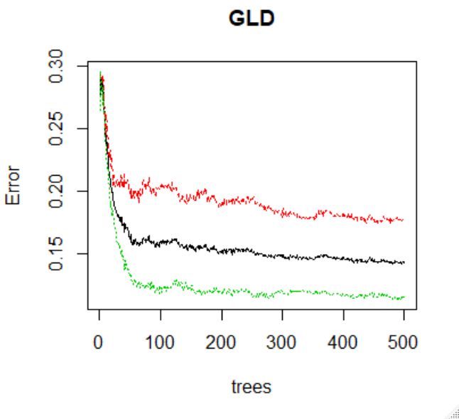
J. Risk Financial Manag. 2021, 14, 198                                                                                               5 of 21

                                         error rate. The classification error rate, E, is the fraction of training observations in a region
                                         that do not belong to the most common class.

                                                                                            max( p̂mk )
                                                                               E = 1−                                                   (2)
                                                                                               k
                                         In Equation (2), p̂mk is the proportion of training observations in the mth region that are
                                         from the kth class. Splits can be classified using a Gini index. The Gini index (G) is defined
                                         as follows.
                                                                                    K
                                                                              G=   ∑ p̂mk (1 − p̂mk )                                   (3)
                                                                                   k =1

                                               The total variance across the K classes can be measured using the Gini index. In this
                                         paper
                                               K = 2 because there are only two classes (stock price direction positive or, not positive).
                                         For small values of p̂mk the Gini index takes on a small value. For this reason, G is often
                                         referred to as a measure of node impurity since a small G value shows that a node mostly
                                         contains observations from a single class. The root node at the top of a decision tree
                                         can be found by trying every possible split of the predictor space and choosing the split
                                         that reduces the impurity as much as possible (has the highest gain in the Gini index).
                                         Successive nodes can be found using the same process and this is how recursive binary
                                         splitting is evaluated.
                                               The entropy (D) is another way to classify splits. The entropy is defined as follows.

                                                                                        K
                                                                             D=−     ∑ p̂mk log( p̂mk )                                 (4)
                                                                                     k =1

                                               The entropy (D), like the Gini index, will take on small values if the mth node is pure.
                                         The Gini index and entropy produce numerically similar values. The classification error is
                                         not very sensitive to the growing of trees so in practice either the Gini index or entropy is
                                         used to classify splits. The analysis in this paper uses the entropy measure.
                                               The process of building a decision tree typically results in a very deep and complex
                                         tree that may produce good predictions on the training data set but is likely to over fit
                                         the data leading to poor performance on unseen data. Decision trees suffer from high
                                         variance which means that if the training data set is split into two parts at random and
                                         a decision tree fit to both parts, the outcome would be very different. Bagging is one
                                         approach to addressing the problem of high variance. Bootstrap aggregation, or bagging
                                         as it is commonly referred to, is a statistical technique used to reduce the variance of a
                                         machine learning method. The idea behind bagging is to take many training sets, build
                                         a decision tree on each training data set, and average the predictions to obtain a single
                                         low-variance machine learning model (James et al. 2013). Since the researcher does not
                                         have access to many training data sets bootstrap replication is used to create many copies of
                                         the original training data set and a decision tree fit to each copy. Averaging the predictions
                                         from bootstrap trees reduces variance, even though each tree is grown deep and has high
                                         variance.

                                         2.3. The Random Forests Method for Prediction
                                              Random forests are an improvement over bagging trees by introducing decorrelation
                                         between the trees (Breiman 2001). As in the case of bagging, a large number of decision
                                         trees are built on bootstrapped training samples. Each time a split in a tree occurs a random
                                         sample of predictors is chosen as split candidates from the full set of predictors. The
                                         number of predictors chosen at random is calculated as the floor of the square root of the
                                         total number of predictors (James et al. 2013). While the choice of randomly choosing
                                         predictors may seem unusual, averaging results from non-correlated trees is more effective
                                         for reducing variance than averaging trees that are highly correlated.
J. Risk Financial Manag. 2021, 14, 198                                                                                            6 of 21

                                         2.4. The Stochastic Gradient Boosting Method for Prediction
                                               Boosting is another way to improve the prediction accuracy of decision trees (James
                                         et al. 2013; Hastie et al. 2009). With boosting, trees are grown sequentially, and each tree is
                                         grown using information from previously grown trees. More specifically, the newly added
                                         decision tree fits the residuals from the current decision tree. The final model aggregates
                                         the results (predicted values) from each step in the sequence. Each tree is a weak learner
                                         but adding many trees together with each tree modelling the errors from the previous
                                         tree can produce a very accurate overall model. Unlike bagging, boosting does not use
                                         bootstrap sampling and instead each tree is fit to a modified version of the original tree
                                         (Friedman 2001). When adding trees, a gradient descent technique is used to minimize the
                                         loss function and this is referred to as gradient boosting. Boosting has tuning parameters
                                         for the number of trees, the shrinkage (learning rate) parameter, the number of splits in
                                         each tree, and the minimum number of observations in each node. Stochastic gradient
                                         boosting is an improvement over gradient boosting because boosting has a tendency to
                                         overfit the data. At the construction of each tree a subsample of the training data drawn at
                                         random without replacement is used to fit the base learner. Stochastic gradient boosting is
                                         used in this paper.

                                         2.5. Model Setup
                                               This paper compares the performance of logit, bagging decision tree, stochastic gra-
                                         dient boosting, and random forests for predicting the price direction of gold and silver
                                         ETFs. For the analysis, 80% of the data was used for training and 20% used for testing. The
                                         logit model uses all the features in predicting price direction. The bagging decision tree
                                         model was estimated with 500 trees. The random forests were estimated with 500 trees and
                                         3 (the floor of the square root of the number of features, 13) randomly chosen predictors
                                         at each split. The results are not sensitive to the number of trees provided a large enough
                                         number of trees are chosen. A very large number of trees does not lead to overfitting, but a
                                         small number of trees results in high test error. In conducting sensitivity analysis, training
                                         control for the random forest and boosting was handled with 10-fold cross validation
                                         with 10 repeats. Stochastic gradient boosting was conducted with 3000 trees, shrinkage
                                         equal to 0.20, an interaction depth of 8, and the minimum number of observations in each
                                         node set to 10. The bag fraction was set at 0.5. Sensitivity analysis showed that these
                                         parameter settings worked well for most forecast horizons. Since boosting has more tuning
                                         parameters than random forests, finding optimal tuning parameter values for each forecast
                                         horizon can be time consuming.
                                               Forecasting accuracy is evaluated using several measures obtained from the confusion
                                         matrix. Accuracy is the number of true positives and true negatives divided by the total
                                         number of predictions. The kappa statistic adjusts accuracy by accounting for the possibility
                                         of a correct prediction just by chance. The positive predictive value measures the proportion
                                         of positive predictions that were correctly classified as positive (true positives divided by
                                         the sum of true positives and false positives). The negative predictive value measures the
                                         proportion of negative predictions that were correctly classified (true negatives divided
                                         by the sum of true negatives and false negatives). All calculations were done in R (R Core
                                         Team 2019) using the random forests machine learning package (Breiman et al. 2018), the
                                         generalized boosted models package (Greenwell et al. 2020) and the caret package (Kuhn
                                         et al. 2020).

                                         2.6. The Data
                                              The data for this study consists of the prices of two popular, US listed, and widely
                                         traded commodity ETFs. The SPDR Gold Shares (GLD) ETF, with an inception date of
                                         18 November 2004, is the most widely traded gold ETF. The GLD ETF is structured as
                                         a trust and holds a specific number of gold bars for each share of the ETF issued. Since
                                         GLD holds physical gold, its share price moves in tandem with the price of gold. GLD
                                         shares were worth one-tenth of the price of gold at inception but this value has eroded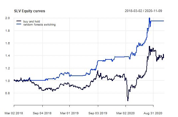
J. Risk Financial Manag. 2021, 14, 198                                                                                         7 of 21

                                       over time because the fund charges a 0.4% annual fee. GLD is an attractive investment for
                                       those who seek exposure to gold but do not want to trade in the commodity market. Silver
                                       prices are measured using the SLV silver trust ETF. SLV consists mostly of silver held by
                                       JPMorgan and a small amount of cash. Like GLD, SLV is passively managed and the price
                                       of SLV closely tracks that of silver. SLV began trading on 21 April 2006. Like GLD, SLV is a
                                       convenient low-cost alternative to investing in the silver futures market.
                                            The daily data set for this study, consisting of 3714 observations, starts on 1 May 2006
                                       and ends on 29 January 2021. The data was collected from Yahoo Finance. Several well-
                                       known technical indicators like the relative strength indicator (RSI), stochastic oscillator
                                       (slow, fast), advance–decline line (ADX), moving average cross-over divergence (MACD),
                                       price rate of change (ROC), on balance volume, money flow index (MFI), Williams accumu-
                                       lation and distribution (WAD), and the 50-day and 200-day moving averages, calculated
                                       from daily data, are used as features in the prediction models. The number of observations
                                       used to estimate the models varies and depends upon the calculation of the technical
                                       indicators (200 days are omitted due to the calculation of the 200-day moving average) and
                                       forecast periods (between 1 and 20 observations are omitted depending upon the forecast
                                       horizon). For a 20-day forecast horizon, there are 3475 observations. The training data
                                       set consists of 2780 observations (80% of the data) and the testing data set contains 695
                                       observations (20% of the data).
                                            The time series pattern of GLD and SLV shows that the ETFs move together (Figure 1).
                                       There are two noticeable peaks in Figure 1. GLD and SLV reached high prices in August of
                                       2011 partially due to debt issues in Europe and the United States and related concerns of
                                       inflation but also because real interest rates turned negative. In late 2020, GLD surpassed
                                       the 2011 peak as the COVID19 pandemic continued. SLV prices increased in 2020 but not
J. Risk Financial Manag. 2021, 14, x FOR
                                       byPEER  REVIEW
                                           enough   to match the previous high set in 2011. Notice that the price of GLD has8 risen
                                                                                                                                of 22
                                       sharply since the onset of the World Health Organization’s declaration of the COVID19
                                       global pandemic (March 2020) which is consistent with gold being used as a hedge in
                                       adverse times.

        Figure 1.
        Figure    This figure
               1. This figure shows
                              shows gold
                                    gold (GLD)
                                         (GLD) and
                                               and silver
                                                   silver (SLV)
                                                          (SLV) ETF
                                                                ETF prices
                                                                    prices across
                                                                           across time.
                                                                                  time. Data
                                                                                        Data are
                                                                                             are sourced
                                                                                                 sourced from
                                                                                                         from Yahoo
                                                                                                              YahooFinance.
                                                                                                                    Finance.

                                              The histograms for the percentage of up days by forecast horizon shows little variation
                                              The histograms for the percentage of up days by forecast horizon shows little varia-
                                         for GLD or SLV (Figure 2). The percentage of up days for GLD never gets higher than 55%
                                         tion for GLD or SLV (Figure 2). The percentage of up days for GLD never gets higher than
                                         while the percentage of up days for SLV never gets higher than 53%.
                                         55% while the percentage of up days for SLV never gets higher than 53%.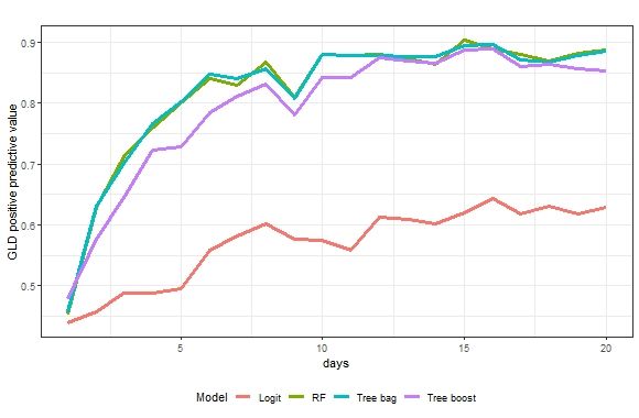
Figure 1. This figure shows gold (GLD) and silver (SLV) ETF prices across time. Data are sourced from Yahoo Finance.

                                              The histograms for the percentage of up days by forecast horizon shows little varia-
J. Risk Financial Manag. 2021, 14, 198                                                                                       8 of 21
                                         tion for GLD or SLV (Figure 2). The percentage of up days for GLD never gets higher than
                                         55% while the percentage of up days for SLV never gets higher than 53%.

      Figure 2. This figure
      Figure          figureshows
                             showshistograms
                                   histogramsofof
                                                gold (GLD)
                                                  gold     andand
                                                       (GLD)   silver  (SLV)
                                                                   silver    ETFETF
                                                                          (SLV) percentage of upofdays.
                                                                                    percentage          Data sourced
                                                                                                   up days.          from Yahoo
                                                                                                             Data sourced  from
      Yahoo  Finance.
      Finance. Author’sAuthor’s own calculations.
                          own calculations.

                                              Descriptive statistics for continuously compounded daily returns show that GLD has
                                         a daily average return of 0.026% while SLV has a daily average return of 0.016% (Table 1).
                                         The coefficient of variation indicates that SLV is more variable. As is common with financial
                                         assets, GLD and SLV each have large kurtosis and non-normally distributed returns.

                                         Table 1. Descriptive statistics of daily returns.

                                                                                             GLD                           SLV
                                          median                                          0.0527                          0.0962
                                          mean                                            0.0262                          0.0159
                                          std.dev                                        1.1613                           2.0436
                                          coef.var                                       44.2617                         128.8832
                                          skewness                                       −0.3345                         −1.0015
                                          kurtosis                                        6.4282                          8.4359
                                          normtest.W                                      0.9394                          0.9147
                                          normtest.p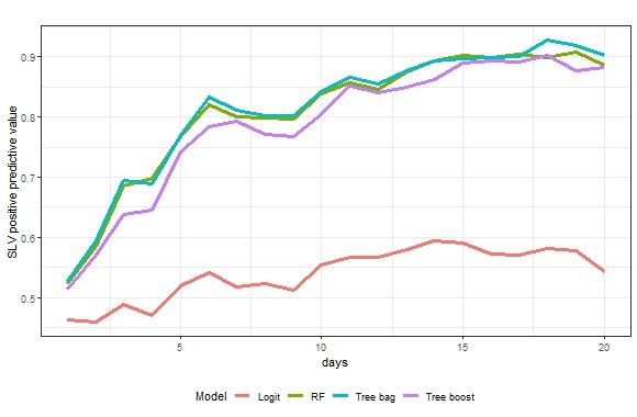
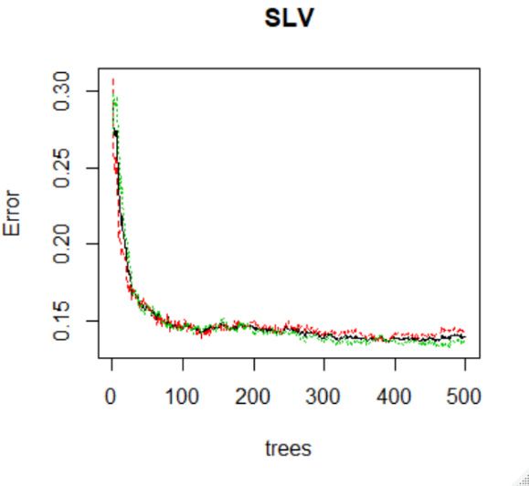
Figure 3 shows how the test error relates to the number of trees. The analysis is conducted
for a 10-step forecast horizon where 80% of the data are used for training and 20% of the
data are used for testing. For each ETF, the test error declines rapidly as the number of
trees increases from one to 100. After 400 trees there is very small reduction in the test
J. Risk Financial Manag. 2021, 14, 198 error. In Figure 3, out of bag (OOB) test error is reported along with test error for 9the up
of 21
and down classification. The results for other forecast horizons are similar to those re-
ported here. Consequently, 500 trees are used in estimating the RFs.
Figure 3. This figure shows RFs test error vs. the number of trees. OOB (Red), down classification (Black), up classification
(Green).
Figure Calculations
3. This figureare doneRFs
shows fortest
predicting
error vs.stock price direction
the number of trees.over
OOBa (Red),
10-stepdown
forecast horizon. (Black), up classification
classification
(Green). Calculations are done for predicting stock price direction over a 10-step forecast horizon.
3. Results
3. Results
This section reports the results from predicting price direction for gold and silver ETFs.
Since this
Thisis section
a classification
reports problem, thefrom
the results prediction accuracy
predicting priceis one of the for
direction most widely
gold andused
silver
measures of forecast
ETFs. Since this is aperformance.
classificationPrediction
problem, accuracy is a proportion
the prediction accuracy is of one
the number of
of the most
true positives
widely used and true negatives
measures divided
of forecast by the total
performance. numberaccuracy
Prediction of predictions. This measure
is a proportion of the
can be obtained
number of truefrom the confusion
positives and true matrix.
negativesPrediction
divided byaccuracy ranges
the total number between 0 and 1
of predictions.
with higher values indicating greater accuracy. Other useful forecast accuracy
This measure can be obtained from the confusion matrix. Prediction accuracy ranges be- measures
like kappa
tween and1how
0 and withwell the models
higher predict thegreater
values indicating up or down classification
accuracy. are also
Other useful available
forecast accu-
and aremeasures
racy reportedlike
since it is interesting
kappa and how wellto see
theifmodels
the forecast accuracy
predict the up for predicting
or down the up
classification
class is similar or different to that of predicting the down class.
Price direction prediction accuracy for GLD (Figure 4) shows large differences between
the logit model and the tree-based classifiers (RF, Tree bag and Tree boost). The prediction
accuracy for logit show that while there is some improvement in accuracy between 1 and
20 days ahead, the prediction accuracy never gets above 0.6 (60%). The prediction accuracy
of the RFs and tree bagging methods show considerable improvement in accuracy between
1 day and 10 days. Prediction accuracy for predicting GLD price direction 10 days into
the future is over 85%. There is little variation in RF and tree bagging prediction accuracy
for predicting price direction between 10 and 20 days into the future and some accuracy
measures are close to 90%. Notice that the prediction accuracy between tree bagging and
RF is very similar. For predicting 15 to 20 days in the future, the RF, bagged, and boosting
models have very similar accuracy. Overall, the RF has the highest accuracy for each of
the forecast periods although for longer dated forecasts (over 10 days) the difference in
accuracy between RF and bagged or boosting is between 1% and 3%.
The patterns of prediction accuracy for the SLV ETF (Figure 5) is very similar to that
which was described for the GLD ETF. RF and tree bagging have the highest accuracy
while logit has the lowest accuracy. Tree boosting accuracy is similar to RF and bagging for
predicting 15 days to 20 days.
Figures 6 and 7 show kappa accuracy values for predicting GLD and SLV price
direction. For GLD the pattern of kappa values in Figure 6 is very similar to the pattern of
accuracy values reported in Figure 4. RF and tree bagging have the highest kappa values
while logit has the lowest. It is also the case that for SLV, RF and tree bagging have the
highest kappa values while logit has the lowest.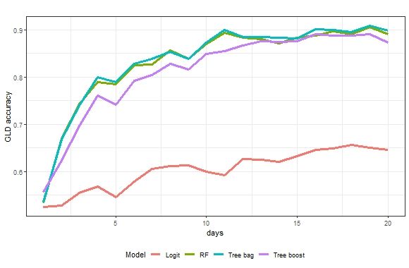
Figures 6 and 7 show kappa accuracy values for predicting GLD and SLV price di-
                                        rection. For GLD the pattern of kappa values in Figure 6 is very similar to the pattern of
                                        accuracy values reported in Figure 4. RF and tree bagging have the highest kappa values
                                        while logit has the lowest. It is also the case that for SLV, RF and tree bagging have the
   J. Risk Financial Manag. 2021, 14, 198                                                                                 10 of 21
                                        highest kappa values while logit has the lowest.

J. Risk Financial Manag. 2021, 14, x FOR PEER REVIEW                                                                      11 of 22

                         Figure 4. This figure shows the multi-period prediction accuracy for GLD price direction.
                      Figure 4. This figure shows the multi-period prediction accuracy for GLD price direction.

                         Figure 5. This figure shows the multi-period prediction accuracy for SLV price direction.
                       Figure 5. This figure shows the multi-period prediction accuracy for SLV price direction.
J. Risk Financial Manag. 2021, 14, 198 11 of 21
Figure 5. This figure shows the multi-period prediction accuracy for SLV price direction.
J. Risk Financial Manag. 2021, 14, x FOR PEER REVIEW 12 of 22
Figure 6. This figure shows the multi-period kappa accuracy for GLD price direction.
Figure 6. This figure shows the multi-period kappa accuracy for GLD price direction.
Figure 7. This figure shows the multi-period kappa accuracy for SLV price direction.
Figure 7. This figure shows the multi-period kappa accuracy for SLV price direction.
In order to determine which variables are most important in the RFs method, variable
In ordermeasures
importance to determine which variables
are provided. areimportance
Variable most important in the RFsby
is ascertained method, variable
using the mean
importance
decrease in measures
accuracy (MD are provided.
accuracy)Variable
and the importance is ascertained
mean decrease in Gini (MD by Gini).
using The
the mean
OOB
decrease in accuracy
data are used (MD the
to conduct accuracy) andFor
analysis. theeach
mean of decrease
GLD andinSLV Giniat(MD Gini). The
a 10-period OOB
forecast
data are used
horizon, MA200, to conduct
MA50, and theWAD
analysis. Forthree
are the eachmost
of GLD and SLV
important at a 10-period
features forecast
in classifying gold
horizon, MA200, MA50, and WAD are the three most important features
and silver price direction because they have the largest values of MD accuracy and MD in classifying
gold
Gini and silver
(Table 2). Inprice direction
additional because
analysis they have
MA200, MA50,theand
largest
WADvalues of important
are also MD accuracy and
features
MD Gini (Table
in classifying gold2).and
In additional
silver priceanalysis
direction MA200, MA50,
for other andhorizons.
forecast WAD are also important
features in classifying gold and silver price direction for other forecast horizons.
Table 2. Variable importance for predicting GLD and SLV price direction.
GLD DOWN UP MD Accuracy MD GiniJ. Risk Financial Manag. 2021, 14, 198 12 of 21
Table 2. Variable importance for predicting GLD and SLV price direction.
GLD DOWN UP MD Accuracy MD Gini
RSI 20.173 29.138 41.748 83.854
StoFASTK 15.784 20.268 28.364 72.086
StoFASTD 16.770 22.636 32.413 73.554
StoSLOWD 20.669 23.290 35.770 79.595
ADX 36.884 45.997 58.702 112.804
MACD 32.026 34.362 49.794 100.971
MACDSignal 37.177 35.449 53.509 109.645
PriceRateOfChange 20.357 27.748 38.655 89.875
OnBalanceVolume 31.622 33.133 56.289 128.120
MA200 46.703 33.859 62.001 160.118
MA50 38.525 35.569 62.455 151.582
MFI 23.270 35.455 44.288 91.704
WAD 34.989 39.088 66.054 131.950
SLV DOWN UP MD Accuracy MD Gini
RSI 21.973 29.103 42.251 80.768
StoFASTK 16.743 23.763 32.791 73.615
StoFASTD 16.543 23.463 32.193 72.895
StoSLOWD 23.559 24.950 37.327 80.689
ADX 39.325 42.789 50.931 114.854
MACD 32.813 39.336 51.095 113.236
MACDSignal 37.227 37.563 51.289 113.466
PriceRateOfChange 20.979 32.039 42.128 92.992
OnBalanceVolume 41.042 34.133 52.971 127.660
MA200 49.461 33.258 64.580 151.835
MA50 39.074 40.194 65.836 150.612
MFI 21.369 26.593 37.392 80.974
WAD 45.073 33.248 58.787 143.667
This table shows the RFs variable importance of the technical analysis indicators measured using mean decrease in
accuracy (MD accuracy) and mean decrease in GINI (MD Gini). Values reported for a 10-period forecast horizon.
The accuracy values shown in Figures 4 and 5 show the overall prediction accuracy. It
is also of interest to see how the prediction accuracy compares between positive prediction
values and negative prediction values. Positive predictive value is the proportion of
predicted positive cases that are actually positive. In other words, when a model predicts
a positive case, how often is it correct? Negative predictive value is the proportion of
predicted negative cases that are actually negative.
The positive prediction values for GLD are shown in Figure 8. The RFs and tree
bagging methods show the highest accuracy across most of the forecast horizons. Tree
boosting accuracy is also high. After just 5 days, the RFs and tree bagging methods have
an accuracy of over 80%. Notice that the logit accuracy never reaches higher than 65%. The
pattern of positive predictive value for the SLV ETF (Figure 9) is similar to that which is
observed for SLV. For each ETF, after 10 days the positive predictive values for RFs and
bagging are above 0.80 and in most cases above 0.85.
Figure 10 shows the negative predictive values for GLD. As in the case of the positive
predictive values for GLD, RFs and tree bagging provide the most accurate negative
predictive values. Tree boosting is slightly less accurate than RFs and tree bagging. The
logit model has the lowest accuracy. Between 1 and 5 days, accuracy increases from 0.5 to
0.8 for the RFs and tree bagging models. After 10 days, negative predictive values for RFs
and tree boosting varies between 0.85 and 0.90. The pattern of negative predictive value
for SLV (Figure 11) is similar to what is observed for GLD (Figure 10). For each of GLD and
SLV, after 10 days the negative predictive values for RFs and bagging are above 0.80 and in
most cases above 0.85.ing accuracy is also high. After just 5 days, the RFs and tree bagging methods have an
accuracy of over 80%. Notice that the logit accuracy never reaches higher than 65%. The
pattern of positive predictive value for the SLV ETF (Figure 9) is similar to that which is
observed for SLV. For each ETF, after 10 days the positive predictive values for RFs and
J. Risk Financial Manag. 2021, 14, 198
bagging are above 0.80 and in most cases above 0.85. 13 of 21
J. Risk Financial Manag. 2021, 14, x FOR PEER REVIEW 14 of 22
Figure 8. This figure shows the multi-period positive predictive values accuracy value for GLD price direction.
Figure 8. This figure shows the multi-period positive predictive values accuracy value for GLD price direction.
Figure 9. This figure shows the multi-period positive predictive values accuracy for SLV price direction.
Figure 9. This figure shows the multi-period positive predictive values accuracy for SLV price direction.
Figure 10 shows the negative predictive values for GLD. As in the case of the positive
predictive values for GLD, RFs and tree bagging provide the most accurate negative pre-
dictive values. Tree boosting is slightly less accurate than RFs and tree bagging. The logit
model has the lowest accuracy. Between 1 and 5 days, accuracy increases from 0.5 to 0.8
for the RFs and tree bagging models. After 10 days, negative predictive values for RFs and
tree boosting varies between 0.85 and 0.90. The pattern of negative predictive value for
SLV (Figure 11) is similar to what is observed for GLD (Figure 10). For each of GLD andJ. Risk Financial Manag. 2021, 14, x FOR PEER REVIEW 15 of 22
J. Risk Financial Manag. 2021, 14, x FOR PEER REVIEW 15 of 22
J. Risk Financial Manag. 2021, 14, 198 14 of 21
Figure 10. This figure shows the multi-period negative predictive value for GLD price direction.
Figure 10. This figure shows the multi-period negative predictive value for GLD price direction.
Figure 10. This figure shows the multi-period negative predictive value for GLD price direction.
Figure 11. This figure shows the multi-period negative predictive value for SLV price direction.
Figure 11. This figure shows the multi-period negative predictive value for SLV price direction.
One concern about predicting stock price direction is that the usual machine learning
Figure 11. This figure shows
One the multi-period
concern negative
about predicting predictive
stock value for SLV
price direction price
is that direction.
the usual machine learning
approach of randomly splitting the data set into training and testing parts may not be
approach of randomly
representative splitting
of time series the datainset
forecasting into training
practice. and testing
The question arisesparts
as to may
how tonotdeal
be
One concern
representative aboutseries
of time predicting stock in
forecasting price direction
practice. is that the arises
usual machinehowlearning
with serial correlation. Bergmeir et al. (2018) show The
thatquestion
in autoregressive as to
models tok-fold
deal
approach
with ofcorrelation.
randomly Bergmeir
splitting the data set into training
that in and testing parts may not be
crossserial
validation is possible so longetasal.the
(2018)
errorsshow autoregressive
are uncorrelated. models
In the approach k-fold
taken in
representative
cross validationof time
is series
possible soforecasting
long as in
the practice.
errors are The question
uncorrelated. arises
In theas to how
approach to deal
taken
this paper, the forecast variable is gold or silver ETF price direction (which is a classification
with serial correlation. Bergmeir et al. (2018) show that in autoregressive models k-fold
rather than regression) and the features are technical indicators, some of which (like the
cross validation is possible so long as the errors are uncorrelated. In the approach taken
MA200) embody a lot of past information on stock prices that helps to mitigate the residualJ. Risk Financial Manag. 2021, 14, 198 15 of 21
serial correlation. To investigate this issue further, a time series cross validation analysis
is conducted where the first 80% of the data are used to fit a RF model to GLD and SLV
and price direction predictions are made. Then, the estimation sample is increased by
one observation and the model re-fit and a new set of forecasts produced. This recursive
approach is used until the end of the data set is reached. This approach is time consuming
because the model is re-fit each time a prediction is made but representative of what an
investor actually does in practice. The results from undertaking this analysis are presented
in Table 3 for a 10- and 20-day GLD and SLV price direction prediction period. The accuracy
values obtained from this approach are referred to as time series cross validation (tsCV).
In comparing CV (the approach of randomly selecting 80% of the data for training
and 20% for testing) with tsCV for predicting GLD price direction over ten days using
RFs, CV accuracy is 0.8698 while tsCV accuracy is 0.8061 (Table 3). In the case of a 20
day prediction for GLD, CV accuracy is 0.8906 and tsCV accuracy is 0.8609. These tsCV
accuracy values are lower (by about 3% to 7%) than the CV values but not by much. This
pattern where tsCV values are slightly less than their corresponding CV values is observed
throughout Table 3. For each accuracy measure, the tsCV values are slightly less than their
corresponding CV values but not enough to diminish the impressive accuracy of the RF
model in predicting stock price direction. Similar results are observed for SLV.
Table 3. Comparing CV with tsCV from random forests prediction.
10 Day 20 Day
GLD CV GLD tsCV SLV CV SLV tsCV GLD CV GLD tsCV SLV CV SLV tsCV
Accuracy 0.8698 0.8061 0.8455 0.7959 0.8906 0.8609 0.9036 0.8522
Kappa 0.7353 0.6085 0.6898 0.5904 0.7791 0.7211 0.8072 0.7043
Pos Pred Value 0.8805 0.7803 0.8379 0.7768 0.8871 0.8434 0.8864 0.8488
Neg Pred Value 0.8621 0.8276 0.8522 0.8132 0.8935 0.8771 0.9213 0.8555
This table shows random forests forecast accuracy values computed from cross validation (CV) and time series cross validation (tsCV) for
gold (GLD) and silver (SLV) price direction.
In order to provide further practical information on the usefulness of using random
forests to predict gold and silver price direction, a comparison was made between a buy
and hold portfolio and a switching portfolio that followed a trading strategy based on
the random forest 20 period price direction forecasts. If the predicted GLD price direction
over the next 20 days was up, then the portfolio was invested in GLD. If the predicted
GLD price direction over the next 20 days was down, then the portfolio was invested
in 3-month US T bills. The chosen portfolio is held for 20 days after which time a new
investment decision was made based on the random forests prediction of GLD price
direction. Over the test period (2 March 2018 to 9 November 2020), the buy and hold
portfolio generated annualized returns, standard deviation, Sharpe ratio, and Omega
ratio values of 12.51%, 14.52%, 0.79, and 1.17, respectively. By comparison, the switching
portfolio generated annualized returns, standard deviation, Sharpe ratio, and Omega ratio
values of 18.56%, 9.53%, 1.84, and 1.67, respectively. The switching portfolio has a higher
Sharpe ratio and Omega ratio indicating better risk and return tradeoffs as compared to
a buy and hold portfolio. It was also the case that for SLV, the switching portfolio has a
higher Sharpe ratio and Omega ratio. Over the test period, the buy and hold SLV portfolio
generated annualized returns, standard deviation, Sharpe ratio, and Omega ratio values
of 13.57%, 29.69%, 0.42, and 1.10, respectively. In comparison, the switching portfolio
generated annualized returns, standard deviation, Sharpe ratio, and Omega ratio values
of 35.31%, 20.01%, 1.70, and 1.66, respectively. Trading costs were not considered in the
portfolio comparisons, but this is not likely a concern because many discount brokers
allow ETF trades at zero or very low (a few basis points) cost. Equity curves are shown in
Figures 12 and 13. Both figures show that the random forests switching portfolio avoids
some large drawdowns.folio comparisons, but this is not likely a concern because many discount brokers allow
35.31%, 20.01%, 1.70, and 1.66, respectively. Trading costs were not considered in the port-
ETF trades at zero or very low (a few basis points) cost. Equity curves are shown in Figures
folio comparisons, but this is not likely a concern because many discount brokers allow
12 and 13. Both figures show that the random forests switching portfolio avoids some
ETF trades at zero or very low (a few basis points) cost. Equity curves are shown in Figures
large drawdowns.
12 and 13. Both figures show that the random forests switching portfolio avoids some
J. Risk Financial Manag. 2021, 14, 198 large drawdowns. 16 of 21
Figure 12. This figure shows GLD equity curves comparing the buy and hold portfolio with the random forests switching
portfolio.
Figure This
12.12.
Figure figure
This shows
figure GLD
shows equity
GLD curves
equity curvescomparing
comparingthe
thebuy
buyand
andhold
holdportfolio
portfoliowith
withthe
the random
random forests
forests switch-
switching
ingportfolio.
portfolio.
Figure 13. This figure shows SLV equity curves comparing the buy and hold portfolio with the random forests switch-
ing portfolio.
To summarize, the main take-away from this research is that RFs and tree bagging
provide much better price direction predicting accuracy then logit. The prediction accuracy
between bagging and RFs is very similar indicating that either method is very useful for
predicting the price direction of gold and silver ETFs. The GLD and SLV price direction
prediction accuracy for RF and tree bagging models is over 80% for forecast horizons of 10
days or more. The positive predictive values and negative predictive values are similarJ. Risk Financial Manag. 2021, 14, 198 17 of 21
indicating that there is little asymmetry between the up and down prediction classifications.
The prediction accuracy from tree boosting is much higher than that of the logit but slightly
lower than that of RF or tree bagging. The prediction accuracy from random forests,
bagging, and boosting, is very similar for forecast horizons greater than 12 days. Boosting
accuracy could be improved by using a more refined tuning grid for each of the 20 forecast
horizons and the two assets but this would involve a tradeoff with respect to increased
computational time since boosting has more tuning parameters than random forests or
bagging and a total of 40 boosted models would need to be trained.
The results in this paper are supportive of the research that shows that predicting
stock price direction can be achieved with high accuracy (Basak et al. 2019; Leung et al.
2000; Nyberg 2011; Nyberg and Pönkä 2016; Pönkä 2016; Ballings et al. 2015; Lohrmann and
Luukka 2019; Sadorsky 2021). Furthermore, the predictive gold price direction accuracy
found in this paper adds to the literature showing the usefulness of using machine learning
methods to predict gold price direction. The gold price direction prediction accuracy
greater than 85% for forecast horizons of 10 to 20 days found in this paper is comparable to
other studies. In predicting one step-ahead weekly gold price changes Parisi et al. (2008)
find that ANN has an accuracy of 61%. Using stacking and hybrid bagging Mahato and
Attar (2014) find one day-ahead gold and silver price accuracy of 85% and 79%, respectively.
Unlike Pierdzioch et al. (2015) and Pierdzioch et al. (2016a) who find that gold price trading
signals generated from regression boosting offer little to no improvement over a buy and
hold strategy, the results of this present paper indicate a trading strategy based on RFs
offers a substantial improvement over a buy and hold strategy.
4. Discussion and Summary
During turbulent economic times or when there is high inflation, investors often use
gold to hedge their investment portfolios. Consequently, it is important for investors to have
accurate forecasts of gold prices. Much of the existing literature on forecasting gold prices
finds that machine learning methods have higher accuracy than econometric methods.
This paper contributes to the literature by comparing the gold and silver price direction
prediction accuracy of several tree-based classifiers. More specifically, RFs, decision tree
bagging, and tree (stochastic gradient) boosting are used to predict gold and silver ETF
price direction over a 20 period forecast horizon. The feature space consists of 13 widely
used technical indicators.
The analysis from this paper yields several important findings. First, RFs and tree
bagging show much better gold and silver price direction prediction accuracy then logit
models. Stochastic gradient boosted models have higher accuracy than logit but not as high
as RFs or tree bagged models. Bagging and RFs produce very similar prediction accuracy
demonstrating that either method is very useful for predicting the price direction of gold
and silver ETFs. RFs stochastic gradient boosting, and tree bagging methods produce
forecast accuracy over 80% for forecast horizons of 10 days or more. For a 20-day forecast
horizon, tree bagging stochastic gradient boosting, and random forests methods produce
accuracy rates of between 85% and 90%. By comparison, logit models have accuracy
rates of between 55% and 60%. These results are in agreement with other research that
shows boosting (Pierdzioch et al. 2015, 2016a, 2016b) and random forests (Liu and Li
2017; Pierdzioch and Risse 2020) to have high accuracy for predicting gold prices. Second,
the positive predictive values and negative predictive values indicate that there is little
asymmetry between the up and down prediction classifications for gold and silver ETFs.
This result is robust to the prediction method used. Third, tree bagging and random forests
offer an attractive combination of accuracy and ease of estimation, for those looking to
forecast the direction of gold and silver prices. Fourth, for each of GLD and SLV, a switching
portfolio that uses the 20 period ahead price direction forecasts from a random forests
model has better risk adjusted returns (a higher Sharpe ratio and Omega ratio) than that of
a buy and hold portfolio.J. Risk Financial Manag. 2021, 14, 198 18 of 21
Future research could expand the set of predictors. This paper used a set of well
known technical indicators for features. The feature space could be expanded to include
additional technical indicators or even macroeconomic variables. Whereas most of the
previous literature uses macroeconomic variables as features to predict gold prices and
this paper uses technical indicators, it may be interesting to do a comparison to see which
group of variables (macroeconomic or technical indicators) is most important in predicting
gold prices.
Funding: This research received no external funding.
Institutional Review Board Statement: Not applicable.
Informed Consent Statement: Not applicable.
Data Availability Statement: Data are publicly available.
Acknowledgments: I thank the anonymous reviewers for their helpful comments. I thank the
Schulich School of Business for internal financial support.
Conflicts of Interest: The author declares no conflict of interest.
Abbreviations
ADX Advance–decline line
ANN Artificial neural network
ANFIS Adaptive neuro-fuzzy inference system
ARIMA Autoregressive integrated moving average
CV Cross validation
ETF Exchange traded fund
ETS Error, trend, seasonality
GARCH Generalized autoregressive conditional heteroskedasticity
GLD Gold shares ETF
Logit Logit regression
LSTM Long short-term memory
MA50 Moving average of length 50
MA200 Moving average of length 200
MACD Moving average cross-over divergence
MFI Money flow index
ML Machine Learning
OBV On balance volume
OOB Out of bag error
RF Random Forest
ROC Price rate of change
RSI Relative strength indicator
SLV Silver shares ETF
SVM Support vector machine
TBATS Exponential smoothing state space model with Box-Cox transformation,
ARMA errors, trend and seasonal components
Tree bag Decision tree bagging
Tree boost Decision tree boosting (Stochastic gradient boosting)
tsCV Time series cross validation
WAD Williams accumulation and distribution
References
Achelis, Steven B. 2013. Technical Analysis from A to Z, 2nd ed. New York: McGraw-Hill Education.
Alameer, Zakaria, Mohamed Abd Elaziz, Ahmed A. Ewees, Haiwang Ye, and Zhang Jianhua. 2019. Forecasting Gold Price Fluctuations
Using Improved Multilayer Perceptron Neural Network and Whale Optimization Algorithm. Resources Policy 61: 250–60.
[CrossRef]
Areal, Nelson, Benilde Oliveira, and Raquel Sampaio. 2015. When Times Get Tough, Gold Is Golden. The European Journal of Finance 21:
507–26. [CrossRef]J. Risk Financial Manag. 2021, 14, 198 19 of 21
Aye, Goodness, Rangan Gupta, Shawkat Hammoudeh, and Won Joong Kim. 2015. Forecasting the Price of Gold Using Dynamic Model
Averaging. International Review of Financial Analysis 41: 257–66. [CrossRef]
Ballings, Michel, Dirk Van den Poel, Nathalie Hespeels, and Ruben Gryp. 2015. Evaluating Multiple Classifiers for Stock Price Direction
Prediction. Expert Systems with Applications 42: 7046–56. [CrossRef]
Basak, Suryoday, Saibal Kar, Snehanshu Saha, Luckyson Khaidem, and Sudeepa Roy Dey. 2019. Predicting the Direction of Stock
Market Prices Using Tree-Based Classifiers. The North American Journal of Economics and Finance 47: 552–67. [CrossRef]
Baur, Dirk G., and Brian M. Lucey. 2010. Is Gold a Hedge or a Safe Haven? An Analysis of Stocks, Bonds and Gold. Financial Review 45:
217–29. [CrossRef]
Baur, Dirk G., and Thomas K. McDermott. 2010. Is Gold a Safe Haven? International Evidence. Journal of Banking & Finance 34: 1886–98.
[CrossRef]
Baur, Dirk G., and Thomas K. J. McDermott. 2016. Why Is Gold a Safe Haven? Journal of Behavioral and Experimental Finance 1: 63–71.
[CrossRef]
Beckmann, Joscha, Theo Berger, and Robert Czudaj. 2015. Does Gold Act as a Hedge or a Safe Haven for Stocks? A Smooth Transition
Approach. Economic Modelling 48: 16–24. [CrossRef]
Bekiros, Stelios, Sabri Boubaker, Duc Khuong Nguyen, and Gazi Salah Uddin. 2017. Black Swan Events and Safe Havens: The Role of
Gold in Globally Integrated Emerging Markets. Journal of International Money and Finance 73: 317–34. [CrossRef]
Bergmeir, Christoph, Rob J. Hyndman, and Bonsoo Koo. 2018. A Note on the Validity of Cross-Validation for Evaluating Autoregressive
Time Series Prediction. Computational Statistics & Data Analysis 120: 70–83. [CrossRef]
Blose, Laurence E. 2010. Gold Prices, Cost of Carry, and Expected Inflation. Journal of Economics and Business 62: 35–47. [CrossRef]
Breiman, Leo. 2001. Random Forests. Machine Learning 45: 5–32. [CrossRef]
Breiman, Leo, Adele Cutler, Andy Liaw, and Matthew Wiener. 2018. RandomForest: Breiman and Cutler’s Random Forests for
Classification and Regression. R Package Version 4.6-14. (version 4.6-14). Available online: https://www.stat.berkeley.edu/
~{}breiman/RandomForests/ (accessed on 30 March 2021).
Bustos, O, and A. Pomares-Quimbaya. 2020. Stock Market Movement Forecast: A Systematic Review. Expert Systems with Applications
156: 113464. [CrossRef]
Ciner, Cetin, Constantin Gurdgiev, and Brian M. Lucey. 2013. Hedges and Safe Havens: An Examination of Stocks, Bonds, Gold, Oil
and Exchange Rates. International Review of Financial Analysis 29: 202–11. [CrossRef]
Friedman, Jerome H. 2001. Greedy Function Approximation: A Gradient Boosting Machine. The Annals of Statistics 29: 1189–232.
[CrossRef]
Gangopadhyay, Kausik, Abhishek Jangir, and Rudra Sensarma. 2016. Forecasting the Price of Gold: An Error Correction Approach.
IIMB Management Review 28: 6–12. [CrossRef]
Greenwell, Brandon, Bradley Boehmke, Jay Cunningham, and G. B. M. Developers. 2020. Gbm: Generalized Boosted Regression
Models (version 2.1.8). Available online: https://CRAN.R-project.org/package=gbm (accessed on 30 March 2021).
Hassani, Hossein, Emmanuel Sirimal Silva, Rangan Gupta, and Mawuli K. Segnon. 2015. Forecasting the Price of Gold. Applied
Economics 47: 4141–52. [CrossRef]
Hastie, Trevor, Robert Tibshirani, and Jerome Friedman. 2009. The Elements of Statistical Learning: Data Mining, Inference, and Prediction,
2nd ed. Springer Series in Statistics; New York: Springer. [CrossRef]
Hillier, David, Paul Draper, and Robert Faff. 2006. Do Precious Metals Shine? An Investment Perspective. Financial Analysts Journal 62:
98–106. [CrossRef]
Hoang, Thi Hong Van, Amine Lahiani, and David Heller. 2016. Is Gold a Hedge against Inflation? New Evidence from a Nonlinear
ARDL Approach. Economic Modelling 54: 54–66. [CrossRef] [PubMed]
Hood, Matthew, and Farooq Malik. 2013. Is Gold the Best Hedge and a Safe Haven under Changing Stock Market Volatility? Review of
Financial Economics 22: 47–52. [CrossRef]
ICE Benchmark Administration Limited (IBA). 2021. Gold Fixing Price 10:30 a.m. (London Time) in London Bullion Market, Based in
U.S. Dollars. FRED, Federal Reserve Bank of St. Louis. FRED, Federal Reserve Bank of St. Louis. 1 April 2021. Available online:
https://fred.stlouisfed.org/series/GOLDAMGBD228NLBM (accessed on 30 March 2021).
Iqbal, Javed. 2017. Does Gold Hedge Stock Market, Inflation and Exchange Rate Risks? An Econometric Investigation. International
Review of Economics & Finance 48: 1–17. [CrossRef]
James, Gareth, Daniela Witten, Trevor Hastie, and Robert Tibshirani. 2013. An Introduction to Statistical Learning: With Applications in R.
Springer Texts in Statistics. New York: Springer. [CrossRef]
Jiang, Zhenlong, Ran Ji, and Kuo-Chu Chang. 2020. A Machine Learning Integrated Portfolio Rebalance Framework with Risk-Aversion
Adjustment. Journal of Risk and Financial Management 13: 155. [CrossRef]
Junttila, Juha, Juho Pesonen, and Juhani Raatikainen. 2018. Commodity Market Based Hedging against Stock Market Risk in Times
of Financial Crisis: The Case of Crude Oil and Gold. Journal of International Financial Markets, Institutions and Money 56: 255–80.
[CrossRef]
Kim, Eun-chong, Han-wook Jeong, and Nak-young Lee. 2019. Global Asset Allocation Strategy Using a Hidden Markov Model. Journal
of Risk and Financial Management 12: 168. [CrossRef]
Koker, Thomas E., and Dimitrios Koutmos. 2020. Cryptocurrency Trading Using Machine Learning. Journal of Risk and Financial
Management 13: 178. [CrossRef]You can also read