Improved nucleosome-positioning algorithm iNPS for accurate nucleosome positioning from sequencing data
←
→
Page content transcription
If your browser does not render page correctly, please read the page content below
ARTICLE
Received 29 Nov 2013 | Accepted 4 Aug 2014 | Published 18 Sep 2014                       DOI: 10.1038/ncomms5909

Improved nucleosome-positioning algorithm
iNPS for accurate nucleosome positioning
from sequencing data
Weizhong Chen1,2,*, Yi Liu1,3,*, Shanshan Zhu1, Christopher D. Green1, Gang Wei1 & Jing-Dong Jackie Han1

Accurate determination of genome-wide nucleosome positioning can provide important
insights into global gene regulation. Here, we describe the development of an improved
nucleosome-positioning algorithm—iNPS—which achieves significantly better performance
than the widely used NPS package. By determining nucleosome boundaries more precisely
and merging or separating shoulder peaks based on local MNase-seq signals, iNPS can
unambiguously detect 60% more nucleosomes. The detected nucleosomes display better
nucleosome ‘widths’ and neighbouring centre–centre distance distributions, giving rise to
sharper patterns and better phasing of average nucleosome profiles and higher consistency
between independent data subsets. In addition to its unique advantage in classifying
nucleosomes by shape to reveal their different biological properties, iNPS also achieves higher
significance and lower false positive rates than previously published methods. The application
of iNPS to T-cell activation data demonstrates a greater ability to facilitate detection of
nucleosome repositioning, uncovering additional biological features underlying the activation
process.

1 Key Laboratory of Computational Biology, Chinese Academy of Sciences-Max Planck Partner Institute for Computational Biology, Shanghai Institutes for
Biological Sciences, Chinese Academy of Sciences, 320 Yue Yang Road, Shanghai 200031, China. 2 Graduate University of Chinese Academy of Sciences,
Beijing 100049, China. 3 Beijing Key Lab of Traffic Data Analysis and Mining, School of Computer and Information Technology, Beijing Jiaotong University,
Beijing 100044, China. * These authors contributed equally to this work. Correspondence and requests for materials should be addressed to J.-D.J.H.
(email: jdhan@picb.ac.cn).

NATURE COMMUNICATIONS | 5:4909 | DOI: 10.1038/ncomms5909 | www.nature.com/naturecommunications                                                        1
                                               & 2014 Macmillan Publishers Limited. All rights reserved.
ARTICLE NATURE COMMUNICATIONS | DOI: 10.1038/ncomms5909
T
he technology of micrococcal nuclease (MNase) digestion of detecting different types of nucleosomes that are associated
combined with high-throughput sequencing (MNase-seq) with different biological properties based on detected nucleosome
is a powerful method to map the genome-wide distribution shapes.
of nucleosome occupancy1–3. Although it has a high demand on The significant increase in accuracy of the iNPS algorithm
sequencing depth, with the promise of probing whole genome- tackled the previously thought major limitations of the MNase-
wide chromatin remodelling events incurred by all transcription seq technology, namely its low resolution and low consistency in
factor binding and chromatin modifications at once and the nucleosome boundary determination5. We now demonstrate that
rapidly decreasing sequencing cost, its popularity has continued the limitations do not lie so much in the technology per se, but
to increase over the years. However, the analysis of nucleosome rather lie in the accuracy of the computational analysis method.
positions is still at its infancy. Nucleosome positioning relies on The iNPS software package is freely downloadable at http://
nucleosome signal coverage, or the frequency distribution formed www.picb.ac.cn/hanlab/iNPS.html.
by MNase digested DNA fragments in a cell population. A
genome location where there is nucleosome occupancy in a
number of cells would have high sequencing read coverage. Thus, Results
the essential principle for nucleosome position detection is to find Improved nucleosome positioning from MNase-seq data. The
the locations where the MNase-seq coverage is enriched. An original NPS algorithm4 mainly contains the following four steps:
effective and efficient strategy is to generate a nucleosome (1) nucleosome scoring for generating a continuous wave-form
sequencing profile that is able to intuitively depict the nucleosome signal for a distribution profile of genome-wide nucleosome
distribution in a wave-form, based on which a peak-calling positioning, (2) wavelet denoising for the preliminary mild
procedure is then used to find the peaks on the wave-form profile. smoothing of the signal waves, (3) Laplacian of Gaussian
Zhang et al.4 have developed an algorithm for nucleosome convolution (LoG) for further smoothing the wave profile and
detection called nucleosome positioning from sequencing (NPS). meanwhile detecting inflection points on the profile as the
In practice, however, the accuracy of the NPS algorithm4 borders of nucleosome peaks and (4) peak filtering based on the
needs much improvement: even if the thresholds for all the cutoff of peak shape and the P-value of Poisson approximation.
filtering steps in the programme are lowered or eliminated In NPS, the original nucleosome profile was generated by
(Supplementary Table 1), many visually obvious nucleosomes still extending each MNase-seq tag from the 50 end by 150 bp towards
could not be detected. To solve this problem, we first identified the 30 position and taking the middle 75 bp as the enriched
the technical problems in NPS contributing to the missing nucleosome signal, thus the nucleosomes were represented by the
or mis-detected nucleosomes; then, we developed a new package peaks on the wave-like original profile. Borders of the nucleosome
‘improved NPS’ (iNPS) by combining the theoretical core peaks, represented by paired inflection points on the smoothed
algorithm of NPS4 with new algorithms to address these profile, could be detected by LoG (Methods). However, the
technical problems. iNPS exhibits a remarkably improved original NPS algorithm cannot precisely determine which pairs of
performance over the original NPS, detecting nucleosomes with inflection points should be selected as final nucleosomes; thus, as
higher quality, a lower false positive rate and stronger association false positives, some mildly concave parts are determined as
with relevant biological events. We also find that NPS’ deficiency nucleosome positions while some obvious sharp peaks are missed
can be largely traced to a hard-coded parameter (Supplementary (Fig. 1a,b). To solve this problem, our iNPS algorithm used a new
Fig. 1a,b); yet, the performance of iNPS is still significantly better method, the first derivative of Gaussian convolution, for detecting
than the ‘customized NPS’ that has the hard-coding problem max/min-extremum points to identify each inflection point pair
fixed (Supplementary Fig. 1c). In addition to the NPS comparison as ‘main’ nucleosome peaks or ‘shoulders’ (Methods, Fig. 2a).
(both default and customized NPS), we further demonstrated an This new step is based on the observation that a sharp peak has a
overall advantage of iNPS over other recent algorithms used for summit on the smoothed profile, while a mildly concave shoulder
nucleosome detection. In particular, iNPS has a unique advantage does not. Then, this step was followed by the next new step for
NPS: results
30
Nucleosome signal
Original scoring profile
25
Detected nucleosomes
20
15
10
5
0
7,734,000 7,735,000 7,736,000 7,737,000 7,738,000 7,739,000
Coordinates of chromosome 1
NPS: nucleosome-detection profile
30
Nucleosome signal
Original scoring profile
25
Nucleosome-detection profile
20
15
10
5
0
7,734,000 7,735,000 7,736,000 7,737,000 7,738,000 7,739,000
Coordinates of chromosome 1
Figure 1 | Nucleosomes detection results by the NPS algorithm. (a,b) The nucleosome detection results of the NPS algorithm on the 7,734,000–
7,739,000 bp region of chromosome 1 (hg18) in resting human CD4 þ T cells. (a) The detected nucleosomes (orange line). (b) The nucleosome-detection
profile (red line): wave-form signal within the detected nucleosomes.
2 NATURE COMMUNICATIONS | 5:4909 | DOI: 10.1038/ncomms5909 | www.nature.com/naturecommunications
& 2014 Macmillan Publishers Limited. All rights reserved.NATURE COMMUNICATIONS | DOI: 10.1038/ncomms5909 ARTICLE
Original nucleosome profile
a c
Gaussian convolution smoothed profile
Max-extremum point
Inflection points
Most-winding position on ‘shoulder’
‘Main’ nucleosome
12
Shoulder After step 3
Nucleosome signal
20
10
15
10
Nucleosome signal
8
5
0
6 148,328,000 148,329,000 148,330,000 148,331,000 148,332,000 148,333000 148,,334,000
Coordinates of chromosome 1
4
Region for the After step 4
determination of
shoulder fate
Nucleosome signal
20
2
15
10
0
5,979,950 5,980,050 5,980,150 5,980,250 5
Coordinates of chromosome 1 0
148,328,000 148,329,000 148,330,000 148,331,000 148,332,000 148,333,000 148,334,000
b Tag Coordinates of chromosome 1
Tag (25 nt) for 5′ of a 5′ 3′
potential nucleosome 3′ 5′ After step 5
150 nt Nucleosome signal 20
Beginning:
15
tag coordinate bed data Extending each tag 5′ 3′
by 150 nt toward 3′ 3′ 5′ 10
Step1: nucleosome scoring
5
75 nt
Wave-form nucleosome 0
signal profile 5′ 3′ 148,328,000 148,329,000 148,330,000 148,331,000 148,332,000 148,333,000 148,334,000
Taking middle 75 nt
3′ 5′
Step2: convolution Coordinates of chromosome 1
Gaussian First derivative LoG Third derivative LoG with a Final results
convolution of gaussian of gaussian smaller deviation
Nucleosome signal
20
convolution convolution
15
Smoothed Max-extremum Inflection Most winding Inflection of more 10
profile Min-extremum position ‘detailed’ wave 5
0
Step3: identifying ‘main’ 148,328,000 148,329,000 148,330,000 148,331,000 148,332,000 148,333,000 148,334,000
nucleosome and ‘shoulder’
Coordinates of chromosome 1
‘Main’ nucleosome candidates
‘shoulder’ candidates d Results by NPS
20
Nucleosome signal
Step 4: Determining whether one shoulder is an independent nucleosome
15
or the dynamic shifting part of the neighboring ‘main’ nucleosome.
10
‘Main’ nucleosome 5
independent ‘shoulder’
integrated nucleosome with shoulder 0
148,328,000 148,329,000 148,330,000 148,331,000 148,332,000 148,333,000 148,334,000
Step 5: adjusting the inflection border. Coordinates of chromosome 1
Nucleosome with more accurate inflection border
Step 6: merging the ‘doublet’.
Nucleosome distribution with more reasonable spacing distance
Step 7: filter some small nucleosome with bad shape.
Final well detected nucleosome
Step 8: statistical test.
Nucleosome with statistical scores
Figure 2 | The algorithmic procedure of iNPS. (a) An illustration of the relationship between a ‘main’ nucleosome and a ‘shoulder’ pattern. (b) Flow chart
of the seven algorithmic steps in iNPS. (c) Step-by-step results of iNPS algorithm. Genomic region 148,328,000–148,334,000 bp in chromosome 1, hg18 of
human resting CD4 þ T cells is used here as an example. Five coloured profile lines are plotted in each panel–blue: original scoring profile, red: Gaussian
convolution smoothed profile, green/purple: LoG convoluted profiles with normal/smaller standard deviations, orange: detected nucleosome peaks. Results
after step 3: detection of candidate ‘main’ nucleosomes/‘shoulders’ (that is, the region of a pair of inflection points with/without max-extreme point
between them). Results after step 4: ‘shoulders’ are determined as independent nucleosomes or dynamic shifting parts of the neighbouring main
nucleosome peaks. Results after step 5: borders of some nucleosomes are adjusted using inflection points identified from the LoG convoluted profiles with
a small standard deviation. Final results: ‘doublets’ patterns are merged and small nucleosome peaks with bad shapes are discarded. (d) The final
nucleosome detection result by NPS on the same genomic region as in c.
NATURE COMMUNICATIONS | 5:4909 | DOI: 10.1038/ncomms5909 | www.nature.com/naturecommunications 3
& 2014 Macmillan Publishers Limited. All rights reserved.ARTICLE NATURE COMMUNICATIONS | DOI: 10.1038/ncomms5909
determining whether a ‘shoulder’ candidate should be an Although the customized NPS shows better performance than
independent nucleosome or merged into the neighbouring ‘main’ the original default NPS (Supplementary Fig. 4a,b versus
nucleosome candidate that has a dynamic shift. Here, the Fig. 1a,b), its performance is still not as good as iNPS, as shown
determination depends on the distance between the shoulder by the distribution of nucleosome width, the distribution of
and the main peaks, their peak height ratio, and, particularly, the neighbouring centre distance, and the consistency between
profile shape features between the nearest inflection point on the resting and activated T cells (Supplementary Fig. 4d,e).
adjacent ‘main’ nucleosome peak and the ‘most-winding’ point
(detected by the third derivative of Gaussian convolution) on the
Quality of genome-wide nucleosome detection. For each
‘shoulder’ (Methods, Fig. 2a, and see examples in Supplementary
detected nucleosome, iNPS scores the confidence level using
Fig. 2). Following these two new major improvements to assure
Poisson test as applied by NPS4 and some other peak-calling
the accuracy of detecting the ‘main’ nucleosome peaks, fine
algorithms for ChIP-seq data, such as MACS7. Unlike NPS and
adjustments were made, including adjusting nucleosome border,
MACS, iNPS not only identifies the tag enrichment within the
merging ‘doublets’, and so on, to resolve minor peaks. On the
peak region (see definition in Methods) for each detected
basis of these improvements, we developed a high-accuracy
nucleosome peak by using upper-tailed Poisson test, but it also
nucleosome-positioning algorithm, the iNPS algorithm (Fig. 2b
identifies the tag depletion within the adjacent ‘valley’ regions
and see an example of step-by-step optimization in Fig. 2c, and
(see definition in Methods) flanking the corresponding
also see an example of the detection result by NPS in Fig. 2d for
nucleosome peak by using lower-tailed Poisson test, resulting
comparison).
in two respective scores ‘ log10(P-value_of_peak)’ and
As a result of introducing these aforementioned steps, the iNPS
‘ log10(P-value_of_valley)’ (see ‘Step 8’ of ‘Algorithmic steps
algorithm detected more nucleosomes than NPS, among which
in iNPS’ in Methods for details).
many obvious sharp peaks missed by NPS are retrieved (Compare
We compared the genome-wide quality of nucleosome output
Fig. 3a,b versus Fig. 1a,b). The full list of genomic coordinates and
by iNPS/NPS by performing Poisson tests for all the detected
shape features of the exemplary nucleosomes detected (Fig. 3a,b)
nucleosomes and by sorting them in decreasing order of
are listed in Supplementary Table 2.
‘ log10(P-value_of_peak)’ and ‘ log10(P-value_of_valley)’,
The distribution of nucleosome ‘width’, as represented by the
respectively. Then, the average log10(P-value) of nucleosomes
length between two inflection points of each detected nucleosome
(per 10,000-sized bins) are plotted for the top 5,000,000 predicted
peak, is plotted in Fig. 3e. It is clear that for most nucleosomes,
nucleosomes by iNPS or NPS on the whole genome of the resting
the ‘width’ is around 70–90 bp, which is consistent with the fact
and activated CD4 þ T cells, respectively (Fig. 4a,b). It is clear
that the middle 75 bp of extended tags was taken to represent
that iNPS outperforms NPS.
the enrichment signal of a nucleosome. The sharp peak of the
In addition, we also evaluated the genome-wide detection
nucleosome width distribution suggests that the majority of
quality of the customized NPS, which is better than the default
the detected nucleosomes are well-positioned and isolated single
NPS (the blue lines versus green lines in Supplementary Fig. 5), as
nucleosomes. Furthermore, the distances between the centres of
expected. However, iNPS still yields overall higher log(P-value)
two neighbouring nucleosomes are around 160–210 bp, peaking
scores (the red lines versus blue lines in Supplementary Fig. 5)
at 180 bp (Fig. 3f). This distance distribution is consistent
than customized NPS, demonstrating the best quality of the
with the fact that nucleosomes are wrapped by a stretch of
detected nucleosomes by iNPS.
147 bp of DNA and separated by B38 bp of linker DNA6. We
then specifically assessed the influence on the distributions
and average nucleosome profiles by different parts of the iNPS Robustness of genome-wide nucleosome detection. To compare
pipeline. By sequentially activating each algorithmic step the robustness of the nucleosome detection by iNPS and NPS, we
(including substeps of Step 6: merging ‘doublets’ and Step 7: randomly and evenly divided the MNase-seq data1 into two
filtering) of iNPS, we observed an increasingly sharper subsets (50% tags in each subset) and obtained two nucleosome
distribution of nucleosome widths (Supplementary Fig. 3a), an detection results by running iNPS and NPS with the same
increasingly better approximation of the neighbouring parameter settings on the two data sets (Methods). Then, the
nucleosome centre distance to the theoretical value (147 bp robustness of the algorithms was quantified by Spearman’s rank
nucleosome þ 38 bp linker) (Supplementary Fig. 3b) and correlation coefficient (SCC) between results on the two
increasingly sharper peaks/better phasing of the average independent subsets of the data to measure their similarity
nucleosome profiles (Supplementary Fig. 3e) from Step 3 to (Methods). Using the DNA fragment of Figs 1 and 3 as an
Step 7 on chromosome 1 of the resting CD4 þ T cells. We also example, the SCC for iNPS-derived profiles (measuring the
observed a mild decreasing of the number of output nucleosomes similarity of the orange and green lines in Fig. 3c) is 0.681, while
through these steps (Supplementary Table 3). The analysis of the the SCC of NPS and customized NPS-derived profiles (measuring
distribution of nucleosome ‘width’ and neighbouring nucleosome the similarity of the orange and green lines in Fig. 3d and
centre distance was also repeated on Chromosome 19 of activated Supplementary Fig. 4c) is 0.417 (NPS) and 0.635 (customized
CD4 þ T cells. The results are qualitatively similar and shown in NPS), respectively.
Supplementary Fig. 3c,d. At the whole-genome level, the differences in SCCs between
In contrast, the original NPS algorithm results in a much more detections on two halves of tags across each of the 24 human
diffuse and flattened distribution of the nucleosome width chromosomes (1–22, X and Y; Fig. 5a, Supplementary Fig. 6 and
(peaking around 70–110 bp) (Fig. 3e) and the neighbouring Supplementary Table 4) are highly significant (average±s.d. are
centre distance (around 130–180 bp, peaking at 150 bp) (Fig. 3f). 0.489±0.029, 0.339±0.039 and 0.444±0.042 for iNPS, NPS, and
Therefore, the comparison suggests that our iNPS algorithm is customized NPS, respectively, with one-tailed paired t-test
able to detect a larger number of well-fixed and well-isolated P ¼ 3.37 10 21 between iNPS and NPS, P ¼ 8.76 10 9
nucleosomes with a more precise centre distance between between iNPS and customized NPS).
neighbouring nucleosomes. Moreover, the distributions generated To further compare the three algorithms using another
by iNPS are more consistent between human resting and independent dataset, we ran a similar analysis on the MNase-
activated CD4 þ T cells compared with those generated by seq data for activated CD4 þ T cells. The SCCs (average±s.d.)
NPS (Fig. 3e,f). for iNPS, NPS and customized NPS are 0.454±0.036,
4 NATURE COMMUNICATIONS | 5:4909 | DOI: 10.1038/ncomms5909 | www.nature.com/naturecommunications
& 2014 Macmillan Publishers Limited. All rights reserved.NATURE COMMUNICATIONS | DOI: 10.1038/ncomms5909 ARTICLE
iNPS: results
Original scoring profile
30 Gaussian convolution smoothed profile
Laplacian of gaussian convolution (LoG)
25
Nucleosome signal
LoG with smaller standard deviation
20 Detected nucleosomes
15
10
5
0
7,734,000 7,735,000 7,736,000 7,737,000 7,738,000 7,739,000
–5
Coordinates of chromosome 1
iNPS: nucleosome detection profile
30 Original scoring profile
Nucleosome signal
25 Nucleosome detection profile
20
15
10
5
0
7,734,000 7,735,000 7,736,000 7,737,000 7,738,000 7,739,000
Coordinates of chromosome 1
iNPS: robustness of identification
Original scoring profile from total tags
30 Nucleosome detection profile from 50% tags
Nucleosome signal
25 Nucleosome detection profile from the other 50% tags
Overlapping peaks
20
15
10
5
0
7,734,000 7,735,000 7,736,000 7,737,000 7,738,000 7,739,000
Coordinates of chromosome 1
NPS: robustness of identification
Original scoring profile from total tags
30
Nucleosome detection profile from 50% tags
Nucleosome signal
25 Nucleosome detection profile from the other 50% tags
20 Overlapping peaks
15
10
5
0
7,734,000 7,735,000 7,736,000 7,737,000 7,738,000 7,739,000
Coordinates of chromosome 1
Distribution of nucleosome ‘width’ Distribution of neighbouring
nucleosome centre distance
4,000,000 5e+05
iNPS: resting CD4+ T cells iNPS: resting CD4+ T cells
iNPS: activated CD4+ T cells iNPS: activated CD4+ T cells
NPS: resting CD4+ T cells NPS: resting CD4+ T cells
NPS: activated CD4+ T cells
4e+05 NPS: activated CD4+ T cells
3e+05
Fraction
Fraction
2,000,000
2e+05
1e+05
0 0e+00
0 20 40 60 80 120 160 200 240 280 0 50 100 150 200 250 300 350 400 450 500
Nucleosome ‘width’ Distance between the centres
of two neighbouring nucleosome
Figure 3 | Improved nucleosome detection results by iNPS. (a–d) Genomic region 7,734,000–7,739,000 bp (hg18) of chromosome 1 in human
resting CD4 þ T cells is shown as an example. (a) Nucleosome detection results by iNPS. (b) The nucleosome detection profile (wave-form signal within
detected nucleosomes) by iNPS (red line). (c) Robustness of iNPS’s detection results. The SCC between nucleosome detection profiles derived from
two sub-data sets (orange and green line) is 0.681. (d) Robustness of NPS’s detection results. The SCC between the nucleosome detection profiles
derived from two sub-data sets (orange and green line) is 0.417. (e) Distribution of nucleosome ‘width’—the length between two inflection points of each
detected nucleosome. (f) Distribution of the distance between the centre points of two neighbouring nucleosomes.
NATURE COMMUNICATIONS | 5:4909 | DOI: 10.1038/ncomms5909 | www.nature.com/naturecommunications 5
& 2014 Macmillan Publishers Limited. All rights reserved.ARTICLE NATURE COMMUNICATIONS | DOI: 10.1038/ncomms5909
−log10(P-value_of_peak) −log10(P-value_of_valley)
80 10
70 9 iNPS: resting CD4+ T cells
iNPS: resting CD4+ T cells 8
Average within each bin for top nucleosomes
Average within each bin for top nucleosomes
60 7 NPS: resting CD4+ T cells
NPS: resting CD4+ T cells
50 6
40 5
30 4
3
20 2
10 1
0 0
0e+00 1e+06 2e+06 3e+06 4e+06 5e+06 0e+00 1e+06 2e+06 3e+06 4e+06 5e+06
70 10
9
60 iNPS: activated CD4+ T cells iNPS: activated CD4+ T cells
8
50 NPS: activated CD4+ T cells 7 NPS: activated CD4+ T cells
40 6
5
30 4
20 3
2
10 1
0 0
0e+00 1e+06 2e+06 3e+06 4e+06 5e+06 0e+00 1e+06 2e+06 3e+06 4e+06 5e+06
Number of nucleosomes ranked by Number of nucleosomes ranked by
‘−log10(P-value_of_peak)’ ‘−log10(P-value_of_valley)’
Figure 4 | Comparing the quality of nucleosomes detected by iNPS and NPS. (a,b) Significance of the peak/valley regions of the detected nucleosomes,
quantified by ‘ log10(P-value_of_peak)’ (a) and ‘ log10(P-value_of_valley)’ (b). The genome-wide MNase-seq data of both resting and activated
CD4 þ T cells are used, and the log(P-value) of the top 5,000,000 nucleosomes ranked by ‘ log10(P-value_of_peak)’ (a) and ‘ log10
(P-value_of_valley)’ (b) are plotted with each bin showing the averaged value of 10,000 nucleosomes.
0.309±0.028 and 0.409±0.036, respectively (one-tailed paired Fig. 7). (3) The s.d. profiles (s.d. of the signals at each 10 bp
t-test P ¼ 1.99 10 24 between iNPS and NPS and P ¼ 2.07 interval within the TSS±2 kb region) by iNPS also have larger
10 11 between iNPS and customized NPS, Fig. 5a, fluctuations than NPS (Fig. 5c), indicating that iNPS is more
Supplementary Fig. 6 and Supplementary Table 4). sensitive in identifying the boundary of nucleosomes with dif-
As background controls, we calculated the SCCs expected from ferent shapes. (4) Similar to these improvements at the TSSs, at
random simulations on chromosome 1 by randomly selecting CTCF-binding sites, both the average and s.d. profiles of
‘detected nucleosomes’ with the same number and total coverage nucleosomes detected by both algorithms support remarkable
length of the two real nucleosome detection ‘subresults’ given by performance improvements of iNPS versus NPS (Fig. 5d, and see
iNPS. They have an average±s.d. of 0.113±0.00046 based on examples in Supplementary Fig. 8).
100 times permutations, giving rise to an empirical P-value
o0.01 for iNPS-derived SCCs. We also performed a genome-
Differential nucleosome positioning. As transcription factor
wide simulation across all the 24 chromosomes (1–22, X and Y),
binding and chromatin remodelling are associated with the
the results are similar to that of the 100 simulations on
change of nucleosome positions or occupancies8,9, we
Chromosome 1 (average SCC±s.d. ¼ 0.105±0.015).
investigated the differentially positioned nucleosomes between
In addition, since nucleosomes are well phased at TSS and
resting and activated CD4 þ T cells (see pipeline in
CTCF-binding sites, we specifically tested the robustness of the
Supplementary Fig. 9). The MNase-seq tags contributing to the
two algorithms in the regions of TSS ( 2,000 to þ 2,000 bp) and
iNPS-detected nucleosomes were selected and inputted into
CTCF ( 1,000 to þ 1,000 bp) in the resting CD4 þ T cell. The
DANPOS10 to obtain differentially positioned nucleosomes
results are similar to those obtained at the single chromosome
(Methods, see the example fragment in Fig. 6a) for the analysis
level (Fig. 5b).
of biological significance (Methods). Among the Top 30 enriched
pathways and transcription factor binding motifs (Fig. 6b),
Average profiles of detected nucleosomes. We then examined several are associated with the T-cell activation, such as
the differences between the average nucleosome detection profiles ‘Sphingosine 1-phosphate (S1P) pathway’11,12, ‘Integrin family
obtained by retaining only the wave-signal within the nucleosome cell surface interactions’13, ‘LKB1 signalling events’14–16,
peaks detected by NPS and iNPS (See the red line in Fig. 1b ‘Proteoglycan syndecan-mediated signalling events’17, ‘TRAIL
versus Fig. 3b for an example). From the average profiles and the signalling pathway’18, ‘VEGF and VEGFR signalling network’19,
s.d. derived from the two algorithms surrounding TSSs (which are ‘IL3-mediated signalling events’20 and motif (‘TGGAAA’) for
further classified according to high, medium and low gene tran- NFAT transcription factor family (nuclear factor of activated T
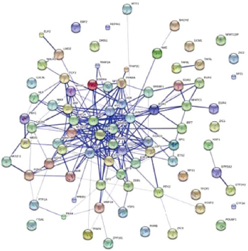
scription levels) and CTCF-binding sites (Fig. 5c,d; see also cells) binding. Moreover, the largest network component
Supplementary Fig. 7 and Supplementary Fig. 8 for more exam- connecting these transcription factors is significantly larger than
ples), we can clearly observe the following key differences random expectation (Methods, Fig. 6c,d, size of 62 nodes versus
between the profiles generated by the two algorithms. (1) For an average of 21 nodes of 10,000 randomly constructed networks
iNPS, the average nucleosome distributions around TSSs at the among the same number of proteins, empirical P-value o10 4).
three expression levels are clearly separated and consistent with Finally, co-citation analysis suggested that iNPS-derived
the expression levels. Even at TSSs of lowly expressed genes, the transcription factors yields high average PubMed counts (6.542)
nucleosome phasing can still be observed, whereas NPS gives no with a significant P-value (Po0.001), showing significant
signal for TSSs of lowly expressed genes, and the differences biological correlation with T-cell activation (Methods).
between the profiles for medium and high levels are not as dis- The same analysis was also performed using the NPS and
tinctive (Fig. 5c). (2) The nucleosome peaks detected by iNPS are customized NPS. Since DANPOS was a necessary algorithmic
sharper than those by NPS (See examples in Supplementary module in the differential analysis, it is interesting to run the
6 NATURE COMMUNICATIONS | 5:4909 | DOI: 10.1038/ncomms5909 | www.nature.com/naturecommunications
& 2014 Macmillan Publishers Limited. All rights reserved.NATURE COMMUNICATIONS | DOI: 10.1038/ncomms5909 ARTICLE
Robustness validation (SCC) on the genome Robustness validation (SCC) around TSS
T_cell_type Resting Resting Activated Activated iNPS NPS
Algorithm iNPS NPS iNPS NPS
Chromosome 1 0.502 0.352 0.467 0.322
Chromosome 2 0.478 0.331 0.441 0.302
Chromosome 3 0.472 0.321 0.436 0.299
Chromosome 4 0.457 0.305 0.424 0.286
Chromosome 5 0.472 0.323 0.436 0.298
Chromosome 6 0.471 0.320 0.434 0.297
Chromosome 7 0.475 0.331 0.440 0.303
Chromosome 8 0.476 0.326 0.440 0.298
Chromosome 9 0.520 0.363 0.489 0.335
Chromosome 10 0.491 0.348 0.453 0.312 1 0.8 0.6 0.4 0.2 0 –0.2
Chromosome 11 0.482 0.343 0.445 0.309
Robustness validation (SCC) around
Chromosome 12 0.472 0.328 0.435 0.299 CTCF-binding sites
Chromosome 13 0.493 0.326 0.465 0.307 iNPS NPS
Chromosome 14 0.507 0.351 0.477 0.323
Chromosome 15 0.528 0.369 0.497 0.340
Chromosome 16 0.517 0.374 0.482 0.337
Chromosome 17 0.490 0.371 0.448 0.320
Chromosome 18 0.471 0.322 0.436 0.296
Chromosome 19 0.494 0.375 0.462 0.327
Chromosome 20 0.499 0.362 0.463 0.322
Chromosome 21 0.526 0.364 0.498 0.334
Chromosome 22 0.560 0.431 0.521 0.365
Chromosome X 0.413 0.267 0.331 0.215
Chromosome Y 0.463 0.224 0.479 0.282
1 0.8 0.6 0.4 0.2 0 –0.3
Nucleosome detection profile near TSS Nucleosome detection profile near CTCF
14
12 5% high, iNPS 5% high, NPS iNPS
5% medium, iNPS 5% medium, NPS NPS
5% low, iNPS 5% low, NPS 12
10
10
8
8
Nucleosome signal
Nucleosome signal
6
6
4
4
2
2
0
0
–2,000 –1,000 0 1,000 2,000
–1,000 –500 0 500 1,000
–2 −2
Distance around TSS −4
Distance around CTCF−binding sites
Figure 5 | Comparison of the robustness and average profiles of nucleosome detection by iNPS and NPS. (a) Heatmap of SCCs between the
‘nucleosome detection profiles’ derived from the two independent subsets containing 50% tags each. SCCs are calculated for the whole genome and for
every chromosome (1–22, X and Y) in both resting and activated CD4 þ T cells. (b) Similar to a, but the SCCs are computed over regions around
TSS/CTCF-binding sites in human resting CD4 þ cells. (c) The average nucleosome detection profiles with s.d. by NPS and iNPS. Three sets of genes are
selected according to high, medium and low transcription levels. For each set, the average and s.d. of the signals at 10 bp resolution are plotted in
warm/cold colours to represent the corresponding nucleosome detection results by iNPS/NPS. The lines in the middle: average profiles of detected
nucleosomes; the lines in the upper and lower parts of the figures are the average±s.d. profiles for the iNPS/NPS results. (d) Average nucleosome profiles
with s.d. at CTCF regions by iNPS/NPS.
whole analysis pipeline using DANPOS alone without any a Likewise, in terms of predicting enriched motifs, the enrich-
priori nucleosome detection steps. ment level by iNPS (Fig. 6b) is again significantly higher than
The differential analysis of nucleosome positioning (see NPS (Supplementary Fig. 10b) and customized NPS
examples in Supplementary Figs 10a, 11a and 12a) between the (Supplementary Fig. 11b), but is slightly lower yet at the same
resting and activated CD4 þ T cells, reveals that the NPS level of DANPOS (Supplementary Fig. 12b).
algorithm only detects a few enriched pathways (fails in this task; For the transcription factor network analysis, the size of the
Supplementary Fig. 10b). Yet all the other three algorithms (iNPS, largest component for the iNPS-derived network (Fig. 6c,d,
customized NPS and DANPOS) basically detect the same set of empirical P-value 10 4) is much larger than that from NPS
enriched pathways, among which iNPS’ enrichment level is the (Supplementary Fig. 10c,d, empirical P-value ¼ 0.0942) and
highest (Fig. 6b, Supplementary Figs 11b and 12b). customized NPS (Supplementary Fig. 11c,d, empirical P-value
NATURE COMMUNICATIONS | 5:4909 | DOI: 10.1038/ncomms5909 | www.nature.com/naturecommunications 7
& 2014 Macmillan Publishers Limited. All rights reserved.ARTICLE NATURE COMMUNICATIONS | DOI: 10.1038/ncomms5909
a
35 Resting T cell
30 Activated T cell
Nucleosome signal
Different detection
25
Significant locations
20
15
10
5
0
7,734,000
–5 7,735,000 7,736,000 7,737,000 7,738,000 7,739,000 7,740,000 7,741,000 7,742,000 7,743,000 7,744,000
–10 Coordinates of chromosome 1
b –log (Hyper FDR Q-Val)
0 10 20 30 40
LKB1 signalling events 6.72
Glypican pathway 7.01
Proteoglycan syndecan-mediated signalling events 7.13
Syndecan-1-mediated signalling events 7.10
Integrin family cell surface interactions 7.18
TRAIL signalling pathway 7.10
Nectin adhesion pathway 7.12
Sphingosine 1-phosphate (S1P) pathway 7.17
Beta1 integrin cell surface interactions 7.16
IGF1 pathway 7.16
VEGF and VEGFR signalling network 7.15
Pathway commons
Alpha9 beta1 integrin signalling events 7.19
signalling events mediated by Hepatocyte Growth Factor Receptor (c-Met) 7.17
signalling events mediated by VEGFR1 and VEGFR2 7.20
IL3-mediated signalling events 7.20
Internalization of ErbB1 7.20
ErbB1 downstream signalling 7.20
Insulin pathway 7.20
Urokinase-type plasminogen activator (uPA) and uPAR-mediated signalling 7.20
S1P1 pathway 7.20
Arf6 downstream pathway 7.20
PDGFR-beta signalling pathway 7.20
Class I PI3K signalling events mediated by Akt 7.20
EGF receptor (ErbB1) signalling pathway 7.20
signalling events mediated by focal adhesion kinase 7.20
Class I PI3K signalling events 7.20
Arf6 signalling events 7.20
Arf6 trafficking events 7.20
mTOR signalling pathway 7.20
PDGF receptor signalling network 7.48
Motif CAGGTG matches TCF3: transcription factor 3 (E2A immunoglobulin enhancer… 36.62
Motif GGGAGGRR matches MAZ: MYC-associated zinc finger protein (purine-binding… 32.38
Motif GGGCGGR matches SP1: Sp1 transcription factor 20.68
Motif CTTTGT matches LEF1: lymphoid enhancer-binding factor 1 19.72
Motif GGGTGGRR matches PAX4: paired box gene 4 17.06
Motif AACTTT (no known TF) 11.99
Motif CACGTG matches MYC: v-myc myelocytomatosis viral oncogene homologue (avian) 11.10
Motif RTAAACA matches FOXF2: forkhead box F2 4.86
Motif CAGCTG matches REPIN1: replication initiator 1
MSigDB predicted promoter motifs
10.77
Motif SNNNCCNCAGGCN matches GTF3A: general transcription factor IIIA 10.60
Motif RNGTGGGC (no known TF) 10.11
Motif GGGSTCWR matches ITGAL: integrin, alpha L (antigen CD11A (p180),… 9.86
Motif RYTTCCTG matches ETS2: v-ets erythroblastosis virus E26 oncogene homolog… 4.40
Motif GCANCTGNY matches MYOD1: myogenic differentiation 1 9.84
Motif GTGGGSGCRRS matches EGR1: early growth response 1 EGR2:… 9.78
Motif GSCCSCRGGCNRNRNN matches GTF3A: general transcription factor IIIA 8.91
Motif CTTTGA matches LEF1: lymphoid enhancer-binding factor 1 4.30
Motif TAATTA matches VSX1: visual system homeobox 1 homolog, CHX10-like… 3.86
Motif CTGCAGY (no known TF) 8.30
Motif TGCCAAR matches NF1: neurofibromin 1 (neurofibromatosis, von… 3.81
Motif CTTTAAR (no known TF) 3.62
Motif CANCCNNWGGGTGDGG (no known TF) 7.98
Motif CNGNRNCAGGTGNNGNAN matches MYOD1: myogenic differentiation 1 7.77
Motif YCATTAA (no known TF) 2.22
Motif TGTTTGY matches FOXA1: forkhead box A1 3.22
Motif TGGAAA matches NFAT NFATC 3.19
Motif TGACAGNY matches MEIS1: Meis1, myeloid ecotropic viral integration site 1… 3.14
Motif RGAGGAARY matches SPI1: spleen focus forming virus (SFFV) proviral… 6.07
Motif TGANTCA matches JUN: jun oncogene 6.30
Motif TTGTTT matches MLLT7: myeloid/lymphoid or mixed-lineage leukemia… 1.94
c d
Distribution of the sizes of the largest
components in randomized networks
0.04
Probability density
0.03
0.02
0.01
0
0 10 20 30 40 50 60 70
The size of the largest component
Figure 6 | Analysis of differential nucleosome positioning between the resting and activated CD4 þ T cells revealed by iNPS. (a) An exemplary
genomic region shows the differential nucleosome positioning based on iNPS’ results in the resting and activated T cells. (b) Top enriched pathways and
‘MSigDB Predicted Promoter Motifs’ associated with genomic regions showing differential nucleosome positioning between the resting and activated
CD4 þ T cells. (c) The network among transcription factors with at least one of the most enriched ‘MSigDB Predicted Promoter Motifs’ (hypergeometric
test FDR o0.001 output by GREAT). (d) Distribution of the sizes of the largest components in randomized networks, with the size of the largest
network component in c marked by the arrow.
8 NATURE COMMUNICATIONS | 5:4909 | DOI: 10.1038/ncomms5909 | www.nature.com/naturecommunications
& 2014 Macmillan Publishers Limited. All rights reserved.NATURE COMMUNICATIONS | DOI: 10.1038/ncomms5909 ARTICLE
10 4), yet comparable with DANPOS (Supplementary Fig. 12c,d, To compare the quality of nucleosome output by different
empirical P-value 10 4). algorithms, we first performed Poisson tests for all the detected
Finally, in the CoCiter’s gene-term analysis, the iNPS-derived nucleosomes. Then, we compared the average log10(P-value) of
transcription factors yield higher average PubMed document nucleosomes (per 10,000-sized bins) for the top 500,000 predicted
counts and more significant P-values than NPS and customized nucleosomes (on Chromosome 1 of the resting CD4 þ T cells) by
NPS, while the two indices for iNPS and DANPOS are comparable. each algorithm. It is clear that iNPS outperformed all other
Taken together, iNPS has better performance in the differential algorithms against which it was compared (Fig. 7a,b). Paired
analysis of nucleosome positioning than NPS and customized t-tests between iNPS and other algorithms show a significantly
NPS. Although DANPOS is specifically designed for this purpose higher log10(P-value) for iNPS detection than other algorithms
and has been shown to be better than other algorithms, we show (Supplementary Table 5). Compared with the differences among
iNPS yields comparable results with DANPOS and it is even different algorithms, there are relatively very small differences
better for predicting biologically significant pathways. among the stepwise results of iNPS, and all these steps yield better
nucleosome detection quality than the other algorithms.
Furthermore, it is also important to show this improvement is
Comparison with other software packages. We also compared not accompanied by an increase in the false positive rates by
iNPS to other algorithms for nucleosome detection, including iNPS. Since it is hard to know the ground truth of nucleosome
NSeq21, NucleoFinder22, nucleR23, NOrMAL24, PING25, positioning in the genome, to quantify the likelihood of different
TemplateFilter26 and DANPOS10, using the resting CD4 þ T algorithms to yield false positive nucleosome predictions, we
cell MNase-seq data for chromosome 1 (ref. 1) (Methods), and generated synthetic MNase-seq data sets by performing rando-
compared them with iNPS (Supplementary Fig. 13). mized simulations (see Supplementary Table 3/Supplementary
NSeq and NucleoFinder detect nucleosomes by finding the Fig. 3e (dotted purple line) for the numbers/sharpness of
centre positions of nucleosomes. These two packages can nucleosome peaks detected by iNPS on the simulated data) and
accurately identify the centre positions of nucleosome peaks used the ratio of the number of detected nucleosomes in the
(Supplementary Fig. 13d,e) but cannot detect the borders of synthetic data versus real data as a surrogate measure of ‘false
nucleosomes. In contrast, iNPS (Supplementary Fig. 13b) pro- positive rates’ (Methods). From the surrogate ‘false positive rate’
vides the range for each nucleosome where the signal is most curves (based on ‘P-value of peak’ or ‘P-value of valley’; Fig. 7c,d),
enriched. nucleR also detects nucleosome positions by finding the it is clear that the iNPS algorithm has the lowest ‘false positive
summit of peaks after noise filtering, but it is unable to separate rates’ among all the algorithms compared. Paired t-tests between
nucleosomes well, resulting in inaccurate border determination iNPS and other algorithms show a significantly lower false
(compare Supplementary Fig. 13b,f). positive rate for iNPS detection than other algorithms
NOrMAL and PING detect nucleosome positions based on (Supplementary Table 6). This firmly demonstrates that iNPS
probabilistic models whose parameters and quantity are esti- enjoys the lowest false positive rates in calling nucleosome peaks.
mated from the MNase-seq data. From the profiles on Moreover, the false positive rates for the intermediate steps of
Chromosome 1, these algorithms apparently cannot match the iNPS are also consistently lower than other algorithms.
other algorithms (Supplementary Fig. 13g,h). In addition, as Specifically, when comparing the performance of these steps,
PING artificially enforced the final width for all the nucleosomes we found that at high x axis values (representing nucleosomes
to be 200 bp in the ‘postPING’ step, it sometimes reports adjacent with lower significance), Step 7’s false positive rates are lower
nucleosomes with overlapping positions (Supplementary than Step 3 when considering peaks yet slightly higher when
Fig. 13h). Moreover, NOrMAL could only detect nucleosomes considering valleys. This observation is consistent with the
on a small chromosomal fragment. In the tests, we had to divide operation that we filter out some low-quality peaks in Step 4–Step
the total sequencing tags of chromosome 1 into 4100 parts at 7 so that the peaks’ quality is improved at the cost of the valleys’.
‘nucleosome deserts’ (long chromosome regions 41,000 bp Moreover, a further detailed comparison of iNPS with the
without MNase-seq coverage) (Methods) and run the programme other packages (Table 1) indicates an overall advantage of iNPS,
on every part, which altogether took 6.5 h to finish. which includes well-detected nucleosomes, unambiguous nucleo-
TemplateFilter identifies nucleosome locations where the some positions with ‘steep slopes’ as clear borders, sharp
forward and reverse read distributions correlate with a series of distributions of neighbouring distances, detailed feature descrip-
model templates. Despite the high accuracy of TemplateFilter tions for each detected nucleosome (for example, height, area
(Supplementary Fig. 13i), it is only able to detect nucleosomes on under the curve and isolated/merged peaks determination) and
a small chromosomal fragment. DANPOS is a pipeline mainly user convenience.
designed for analysing dynamic nucleosome positioning and
occupancy. It also contains a crude peak-calling algorithm inside
which it cannot determine the borders of nucleosomes precisely. Four types of nucleosomes identified by iNPS. According to the
It can well detect sharp peaks, but it is unable to exclude noise shapes of detected nucleosome peaks, iNPS is able to identify four
between peaks (Supplementary Fig. 13j). main types of nucleosomes—‘MainPeak’ (an isolated ‘main’
As more quantitative measurements, we compared the nucleosome peak), ‘MainPeak þ Shoulder’ (a ‘main’ peak asso-
distribution of nucleosome widths (Supplementary Fig. 13k) and ciated with a ‘shoulder’), ‘MainPeak:doublet’ (a merged ‘doublet’)
the distribution of distances between two neighbouring nucleo- and ‘Shoulder’ (an independent ‘shoulder’). Each type of
some centres (Supplementary Fig. 13l) for the nucleosome nucleosome has a distinctive distribution of nucleosome width
positioning results on chromosome 1 in resting CD4 þ T cells. (length between two inflection points of each detected nucleo-
While iNPS generated a nucleosome width distribution between some peak; Supplementary Fig. 14a,b), and each kind of neigh-
70 and 90 bp (peaking at 80 bp; Supplementary Fig. 13k) and a bouring nucleosome pair (four nucleosome types have altogether
neighbouring nucleosome centre distance between 160 and 210 bp 10 kinds of neighbouring nucleosome pair) has a distinct dis-
(peaking at 180 bp; Supplementary Fig. 13l), the other algorithms tribution of neighbouring centre distance (Supplementary
generated more diffuse and flattened distributions with ambiguous Fig. 14c,d). Compared with the ‘MainPeak’ nucleosomes, which
maximum (except the distribution of the neighbouring nucleo- account for B80% of the detected nucleosomes, the ‘Shoulder’
some centre distances generated by DANPOS). nucleosomes have a shorter width and closer distance to nearby
NATURE COMMUNICATIONS | 5:4909 | DOI: 10.1038/ncomms5909 | www.nature.com/naturecommunications 9
& 2014 Macmillan Publishers Limited. All rights reserved.ARTICLE NATURE COMMUNICATIONS | DOI: 10.1038/ncomms5909
−log10(P−value_of_peak) −log10(P−value_of_valley)
(chromosome 1, resting CD4+ T cells) (chromosome 1, resting CD4+ T cells)
25 iNPS: after step 3 6 iNPS: after step 3
iNPS: after step 4 iNPS: after step 4
iNPS: after Step 5 iNPS: after step 5
iNPS: after step 6 5 iNPS: after step 6
20
Average within each bin for
iNPS: final results
Average within each bin
iNPS: final results
for top nucleosomes
Default NPS Default NPS
top nucleosomes
Customized NPS
4
Customized NPS
15 nucleR nucleR
NOrMAL 3 NOrMAL
PING PING
10 TemplateFilter TemplateFilter
DANPOS 2 DANPOS
5
1
0 0
0e+00 1e+05 2e+05 3e+05 4e+05 5e+05 0e+00 1e+05 2e+05 3e+05 4e+05 5e+05
Number of nucleosomes Number of nucleosomes ranked
ranked by ‘−log10(P−value_of_peak)’ by ‘−log10(P−value_of_valley)’
False positive based on ‘P−value of peak’ False positive based on ‘P−value of valley’
(chromosome 1, resting CD4+ T cells) (chromosome 1, resting CD4+ T cells)
iNPS: after step 3
iNPS: after step 3 2.0 iNPS: after step 4
iNPS: after step 5
iNPS: after step 4
2.0 iNPS: after step 6
iNPS: after step 5 iNPS: final results
iNPS: after step 6 Default NPS
1.5 Customized NPS
False positive rate
False positive rate
nucleR
1.5 NOrMAL
PING
TemplateFilter
1.0 DANPOS
1.0 iNPS: final results
Default NPS
Customized NPS
nucleR 0.5
0.5
NOrMAL
PING
TemplateFilter
0.0 DANPOS 0.0
0
200,000
400,000
600,000
800,000
0
1,000,000
1,200,000
600,000
800,000
200,000
400,000
1,000,000
1,200,000
Number of nucleosomes Number of nucleosomes
ranked by ‘−log10(P−value_of_peak)’ ranked by ‘−log10(P−value_of_valley)’
Figure 7 | Comparison of the nucleosome detection quality and false positive rates among different steps of iNPS and other algorithms on
chromosome 1 of the resting CD4 þ T cells. Solid lines: iNPS and other algorithms; Dotted lines: the stepwise results of iNPS. (a,b) Significance of the tag
distribution in peak or valley of detected nucleosomes. (a) Peak regions, quantified by ‘ log10(P-value_of_peak)’ and (b) valley regions, quantified by
‘ log10(P-value_of_valley)’. The top 500,000 nucleosomes output by each algorithm are used and the average log(P-value) per 10,000 nucleosomes
are plotted. (c,d) Comparison of false positive rate based on ‘P-value of peak’ (c) and ‘P-value of valley’ (d), evaluated by comparing the number of
nucleosomes detected from real and randomly simulated MNase-seq data sets. The x axis is the number of top ranked nucleosomes predicted by each
algorithm, and the y axis is the false positive rates. Each point on a curve is the average false positive based on 10 times of simulation, and the s.d.
is not plotted since they are very small (about 10 4–10 3). Significance of the differences of nucleosome detection quality (a,b)/false positive rates (c,d)
between different algorithms is quantified by paired t-tests, shown in Supplementary Tables 5 and 6, respectively.
nucleosomes, while the ‘MainPeak þ Shoulder’ and ‘Main- distribution has a unique phase for the doublet nucleosomes: for
Peak:doublet’ nucleosomes are wider between inflection bound- each of the two types of nucleosomes, the highest transcription
aries and farther from nearby nucleosomes (Supplementary factor motif density peaks overlap with the nucleosomes (green
Fig. 14c,d). These observations suggest that these non-‘Main- and red lines in Fig. 8b), while for ‘MainPeak’ nucleosomes, or
Peak’ nucleosomes are perhaps associated with nucleosome other well-phased nucleosomes on either side of any nucleosome,
destabilization. As the histone variant H2A.Z27–29 or the average transcription factor motif density profile has two high
transcription factor binding30–33 often induces nucleosome shift peaks at the valley flanking the nucleosome (Fig. 8b). This
or destabilization, we examined the average H2A.Z profiles and suggests that doublets are more likely to be associated with ‘on-
average transcription factor motif density profiles around every site’ transcription factor binding on the nucleosome, consistent
nucleosome ( 1,000 to þ 1,000 bp) for each type of nucleosome with their role as mobile or destabilized nucleosomes. We further
(Methods; Fig. 8). Unlike the other two types, the average separately examined the average H2A.Z profiles and average
profiles for the doublet types (‘MainPeak þ Shoulder’ and transcription factor motif density profiles for nucleosomes of
‘MainPeak:doublet’) have an H2A.Z/nucleosome peak at the different distances to the nearest TSS (r2, 2–10, 10–100 and
centre position (see the green and red lines in Fig. 8a), indicating 4100 kb; Supplementary Figs 15 and 16). These profiles are
enrichment of H2A.Z at these two types of non-‘MainPeak’ consistent with the patterns observed based on the total
nucleosomes. Moreover, the transcription factor motif density nucleosome profiles. Taken together, the nucleosome types
10 NATURE COMMUNICATIONS | 5:4909 | DOI: 10.1038/ncomms5909 | www.nature.com/naturecommunications
& 2014 Macmillan Publishers Limited. All rights reserved.NATURE COMMUNICATIONS | DOI: 10.1038/ncomms5909 ARTICLE
Table 1 | Comparison of iNPS with other nucleosome-positioning algorithms.
iNPS Default NPS Customized NSeq NucleoFinder nucleR NOrMAL PING TemplateFilter DANPOS
NPS
Clear borders Yes Yes Yes No No No* Yes Now Yes Yes
for nucleosomes
AUC for Yes No No No No No No No No No
nucleosome
peaks
Accuracy Yes No Yes Yes Yes No No No Yes Yes
Isolated/ Yes No No No No No No No No No
merged peaks
determination
Nucleosomes in 985,407 589,604z 842,318z 557,829z Unknown 1,260,733y 654,069 537,280 867,681 943,273
chr1
Neighbouring 160–210 bp 140–180 bp 140–180 bp 115–135 bp Unknown 100–175 bp 180–270 bp 135–175 bp 130–170 bp 170–220 bp
nucleosome (180 bp) (160 bp) (160 bp) (125 bp) (120 bp) (235 bp) (150 bp) (145 bp) (190–195 bp)
centre (Peak
maximum)
User
convenience
Run time on B1.7 h o1 h o1 h B5 min|| 3h 10 h 6.5 hz 0.5 h|| 7 hz o1 h
chr1
Depended Python Python, Python, Java R with R withE10 Linux with R withE30 Linux Python, R,
environment cython, cython, multicore packages g þþ packages rpy2, numpy
NumPy, NumPy,
Pywavelets Pywavelets
Automation Yes Yes Yes Yes Yes No Noz No Noz Yes
Optimized Yes No No Yes Yes No Yes Yes Yes No
parameters
Output wave- Yes Yes Yes Partly No Yes No Partly No Yes
form profile
AUC, area under the curve; chr, chromosome.
*nucleR assumes the detected nucleosomes are 147 bp long.
wThe size of all the output nucleosomes by PING is 200 bp after the ‘postPING’ step, resulting in overlap of some nucleosomes with their neighbours.
zTotal nucleosomes detected without P-value or FDR cutoff.
ySince nucleR was unable to well distinguish the nucleosome boundaries, too many false positives were detected.
||Programme was run with 20 CPU cores.
zDue to the limited data processing capacity of NOrMAL and TemplateFilter, the input data was manually divided into 115 parts, and the detection was done part-by-part.
0.0095 ‘Mainpeak’ 8
‘MainPeak’
0.08 ‘MainPeak+Shoulder’ 7
6
‘MainPeak:doublet’ 0.0085 5
‘Shoulder’ 4
0.06 3
0.0075 2
H2A.Z signal
0.0080
Nucleosome signal (dotted line)
‘Mainpeak+shoulder’ 8
7
TF-motif density (solid line)
0.04 0.0075 6
5
0.0070 4
3
0.02 0.0065 2
0.0075 ‘Mainpeak:doublet’ 7
6
0.00 0.0070 5
−1,000 −500 0 500 1,000 0.0065 4
3
Distance to nucleosome 0.0060 2
0.0080 ‘Shoulder’ 8
7
0.0075 6
5
0.0070 4
3
0.0065 2
−1,000 −500 0 500 1,000
Distance to nucleosome
Figure 8 | Average H2A.Z and transcription factor motif density profiles for the four types of nucleosomes identified by iNPS. (a) Average H2A.Z
profiles. (b) Average transcription factor (TF) motif density profiles (solid lines). Nucleosome profiles are also shown as dotted lines for TF-motif
enrichments comparison in b.
identified by iNPS based on detected nucleosome shapes also sequence tags is a key step. In iNPS, we followed NPS to represent
implicate different biological functions of nucleosomes. the core part of a nucleosome using the middle 75 bp in each
150 bp-extended tag, since taking either full length or the middle
point would probably result in a decrease of nucleosome resolution
Discussion (Supplementary Fig. 13a) or a decrease of signal enrichment level.
Deep genome sequencing after MNase digestion (MNase-seq) has To facilitate further peak calling, a step of profile smoothening
been an effective way for inferring a genome-wide map of could reduce noise. There are various kinds of tactics available,
nucleosome positions, in which deriving nucleosome profiles from such as Fast Fourier Transform methods used in nucleR23 and the
NATURE COMMUNICATIONS | 5:4909 | DOI: 10.1038/ncomms5909 | www.nature.com/naturecommunications 11
& 2014 Macmillan Publishers Limited. All rights reserved.ARTICLE NATURE COMMUNICATIONS | DOI: 10.1038/ncomms5909
wavelet- and convolution-based method used in NPS4. In accuracy with clear nucleosome borders, higher detection cover-
practice, we found that the Gaussian convolution method alone age with better quality, lower false positive rates, more uniform
was sufficiently effective for profile smoothing. In addition, neighbouring distance, more detailed result descriptions for
combining Gaussian convolution with basic derivative operations downstream analysis and better user convenience.
(convolution with first, second (Laplacian) and third derivatives
of Gaussian) in iNPS could correspondingly detect max/min- Methods
extremum points (summit/valley), inflection points and the most Data sets and software package. Tag coordinate bed files for MNase-digest
winding positions on the smoothed profiles. These key locations sequencing data of human CD4 þ T cells1 was downloaded from National Heart
Lung and Blood Institute (NHLBI), National Institutes of Health (NIH) (http://
play important roles in nucleosome positioning: the inflection dir.nhlbi.nih.gov/papers/lmi/epigenomes/hgtcellnucleosomes.aspx). Tag coordinate
points identify borders of nucleosomes, the max/min-extremum bed file for H2A.Z ChIP-seq data of human CD4 þ T cells34 was downloaded from
points help to distinguish the ‘main’ nucleosome candidates and NHLBI, NIH (http://dir.nhlbi.nih.gov/papers/lmi/epigenomes/hgtcell.aspx). Gene
the most winding positions play a part in fate-decision for the expression microarray data for human CD4 þ T cells1 was downloaded from the
GEO repository with accession number GSE10437. Coordinate information of TSSs
‘shoulder’ candidates. was downloaded from the UCSC repository (http://hgdownload.cse.ucsc.edu/
After finishing the basic step of nucleosome detection, iNPS goldenPath/hg18/database/refFlat.txt.gz) on 30 July 2012. The coordinate
adjusts nucleosome borders of the preliminary results, merges information of CTCF-binding sites35 was downloaded from http://bioinformatics-
closely located ‘doublets’ and filters some small peaks with bad renlab.ucsd.edu/rentrac/wiki/CTCF_Project, and converted into hg18 system.
shapes. With these additional procedures, the final results show Human protein network data was downloaded from STRING (version 9.05)
(ftp://string-db.org/STRING/9.05/protein.links.detailed.v9.05.human_only.txt.gz) on
increased accuracy (Fig. 3a,b) together with a sharper distribution 5 August 2013. A predicted transcription factor motif coordinates map for
of nucleosome width and neighbouring distances (Fig. 3e,f). lymphoblastoid cell lines36 was downloaded from the ‘CENTIPEDE’ website (http://
Different from other packages, iNPS uses both statistical scores centipede.uchicago.edu/data/CentipedeAllP99.bed.gz). For software packages, NPS
(‘ log10(P-value_of_peak)’ and ‘ log10(P-value_of_valley)’) (Nucleosome Positioning from Sequencing), version 1.3.2, was downloaded from
http://liulab.dfci.harvard.edu/NPS/ on 1 December 2011. NSeq21 was downloaded
and geometrical features (peak height, peak width and area from https://github.com/songlab/NSeq on 19 April 2013. NucleoFinder22 was
under the curve) of the detected nucleosome peaks to quantify the downloaded from https://sites.google.com/site/beckerjeremie/ on 22 April 2013.
confidence level of each nucleosome, which not only increases the nucleR23, version 1.9.0, was downloaded from http://bioconductor.org/packages/
detection consistency but also provides further biological insights devel/bioc/html/nucleR.html on 25 April 2013. NOrMAL24 version beta2, was
downloaded from http://code.google.com/p/normal-nucleosome-mapping-
such as the distinction between well-fixed nucleosomes and algorithm/downloads/list on 22 April 2013. PING25, Version 2.3.1, was downloaded
potentially destabilized nucleosomes. from http://www.bioconductor.org/packages/devel/bioc/html/PING.html on 28 April
On the basis of the whole genome-wide nucleosome position- 2013. TemplateFilter26 was downloaded from http://compbio.cs.huji.ac.il/
ing by iNPS in both resting and activated CD4 þ T cells, we NucPosition/TemplateFiltering/Home.html on 22 April 2013. DANPOS10, version
found that the differentially positioned nucleosomes are highly 2.1.2, was downloaded from http://code.google.com/p/danpos/ on 14 May 2013.
enriched for immune pathways (Fig. 6b) and for transcription
factors, which coherently interact with each other (Fig. 6c), which Algorithmic steps in iNPS. iNPS is developed based on Zhang et al.’s methods4,
from which we adopted two key steps—‘nucleosome scoring’ (generating
are otherwise not possible to identify using NPS (Supplementary continuous wave-form signal for genome-wide nucleosome positioning) and
Fig. 10b,c). This highlights the great importance of precisely ‘Laplacian of Gaussian (LoG) convolution’ (detecting inflection points to find
detecting the nucleosome positions. candidate nucleosomes). We then designed and integrated our new steps to develop
We also compared the consistency and boundary resolution of the iNPS algorithm (Fig. 2b), including the following eight steps.
Step 1—nucleosome scoring. Wave-form nucleosome signal profile, with a
nucleosome detection between iNPS and NPS. In terms of resolution of 10 bp, is obtained by extending each sequencing tag (each tag is
consistency, our iNPS algorithm could detect the nucleosome- extended from its 50 end by 150 bp (B1 nucleosome length) toward its 30 direction
positioning profiles between two independent subsets of MNase- (Fig. 2b inset)), of which the middle 75 nt was taken to represent the enrichment of
seq data with a SCC 0.489±0.029 (average±s.d. for the 24 nucleosome signal. The nucleosome score at each coordinate is summed by all the
extended tags covering this coordinate, and these tags on either sense or antisense
chromosome in resting CD4 þ T cells), which increased strand contribute equally to the score at this coordinate.
significantly from NPS’s 0.339±0.039 (P ¼ 3.37 10 21; Step 2—Gaussian convolution. Discrete Gaussian convolution is performed as
Fig. 5a). In terms of boundary resolution, the nucleosome equation (1) to smoothen the wave-form nucleosome signal profile:
detected by iNPS has a much sharper width distribution than xX
þ 3s
1 ðx kÞ2
NPS, with a twofold peak height of that by NPS, and an average yðxÞ ¼ f ðxÞgðxÞ ¼ pffiffiffiffiffiffiffiffiffiffi f ðkÞe 2s2 ð1Þ
2ps2 k¼x 3s
width±s.d. of 84.312±15.056 bp and 83.960±15.150 bp (around
the peak-region of 40–130 bp for resting and activated T cells, where x is the coordinate on the genome, f(x) is the original nucleosome scoring at
respectively) by iNPS versus 89.913±17.778 bp and coordinate x, y(x) is the smoothed signal at coordinate x, deviation s ¼ 3 and the
range (x–3s, x þ 3s) is used for profile smoothening. s ¼ 1 is also used to generate
88.864±17.614 bp by NPS, indicating significantly reduced another mildly smoothed profile for the ‘borders adjustment’ in Step 5. Besides this
variation of the iNPS detection results (F-test P-value ¼ 0; basic step, convolutions with Gaussian derivatives are also performed to detect
Fig. 3e). Thus, a better nucleosome detection algorithm, such as important sites on the wave-form profile:
iNPS, will definitely enhance the application of MNase-seq 1. Convolution with the first derivative of Gaussian is used as equation (2) to
detect max/min-extremum points of the smoothed profile (where the convolution
technology in various fields of biological research. results ¼ 0, s ¼ 3):
Finally, a good software tool should be convenient for users. A
xX
þ 3s
primary requirement is the direct applicability of the software on d d 1
ðf ðxÞgðxÞÞ ¼ f ðxÞ gðxÞ ¼ pffiffiffiffiffiffiffiffiffiffi2
xk ðx kÞ2
f ðkÞ 2 e 2s2 ð2Þ
a large chromosome and preferably a whole genome. In this dx dx 2ps k¼x 3s s
respect, iNPS successfully performed nucleosome positioning on 2. Convolution with the second derivative (Laplacian) of Gaussian (LoG) is used
the whole human genome but NOrMAL and TemplateFilter as equation (3) to detect inflection points of the smoothed profile (where the
could not. Furthermore, the installation and execution of iNPS is convolution results ¼ 0, s ¼ 3), representing the candidate position of nucleosome
peaks (See the formula below). This operation is also repeated for (s ¼ 1) to detect
easy on the Linux system. another set of inflection points on the mildly smoothed profile for border
Taken together, the improved iNPS algorithm, compared with adjustment in Step 5.
the original NPS, showed a significantly higher sensitivity,
d2 d2
detection quality, robustness and lower false positive rate in ðf ðxÞgðxÞÞ ¼ f ðxÞ 2 gðxÞ
dx2 dx
detecting genome-wide nucleosome positions from the MNase- xX
þ 3s
seq data. Further comparison of iNPS with other software 1 ðx kÞ2 1 ðx kÞ2
¼ pffiffiffiffiffiffiffiffiffiffi2 f ðkÞ 4
2 e 2s2 ð3Þ
2ps k¼x 3s s s
packages indicated an overall advantage of iNPS, including higher
12 NATURE COMMUNICATIONS | 5:4909 | DOI: 10.1038/ncomms5909 | www.nature.com/naturecommunications
& 2014 Macmillan Publishers Limited. All rights reserved.You can also read