Eddy induced trapping and homogenization of freshwater in the Bay of Bengal
←
→
Page content transcription
If your browser does not render page correctly, please read the page content below
Eddy induced trapping and homogenization of freshwater in the Bay of Bengal

                                                                             Nihar Paul1 , Jai Sukhatme1,2 , Debasis Sengupta1,2 and Bishakdatta Gayen1,3
                                                                  1
                                                                      Centre for Atmospheric and Oceanic Sciences, Indian Institute of Science, Bangalore - 560012, India.
                                                                       2
                                                                         Divecha Centre for Climate Change, Indian Institute of Science, Bangalore - 560012, India. and
                                                                                  3
                                                                                    Mechanical Engineering Department, University of Melbourne, Australia.

                                                               Freshwater from rivers influences Indian summer monsoon rainfall and regional tropical cyclones by shallowing
                                                               the upper layer and warming the subsurface ocean in the Bay of Bengal. Here, we use in situ and satellite data
                                                               with reanalysis products to showcase how river water can experience a significant increase in salinity on sub-
                                                               seasonal timescales. This involves the trapping and homogenization of freshwater by a cyclonic eddy in the Bay.
                                                               Specifically, in October 2015, river water is shown to enter a particularly long-lived eddy along with its attracting
                                                               manifolds within a period of two weeks. The eddy itself is quite unique in that it lasted for 16 months in the
arXiv:2101.06058v1 [physics.ao-ph] 15 Jan 2021

                                                               Bay where average lifespans are of the order of 2-3 months. This low salinity water results in the formation of a
                                                               highly stratified surface layer. In fact, when freshest, the eddy has the highest sea-level anomalies, spins fastest,
                                                               and supports strong lateral gradients in salinity. Subsequently, observations reveal progressive homogenization
                                                               of salinity and relaxation of sea-level anomalies and salinity gradients within a month. In particular, salty water
                                                               spirals in, and freshwater is pulled out across the eddy boundary. Lagrangian experiments elucidate this process,
                                                               whereby horizontal chaotic mixing provides a mechanism for the rapid increase in surface salinity on the order
                                                               of timescale of a month. This pathway is distinct from vertical mixing and likely to be important in the eddy-rich
                                                               Bay of Bengal.

                                                                        I.   INTRODUCTION                                   an increase in saltiness with southward advection [31]. In this
                                                                                                                            context, the role of eddies in stirring the salinity field has been
                                                                                                                            recognized [20, 28, 53]. In fact, eddy induced variability in
                                                 The Bay of Bengal (BoB) is a semi-enclosed basin lying                     sea surface salinity has been recently observed in other ocean
                                                 between 6-22◦ N, 80-100◦ E, connected to the equatorial In-                basins such as the tropical Pacific [16] and the Arabian Sea
                                                 dian Ocean to the south. The Ganga-Brahmaputra-Meghna                      [63].
                                                 (GBM), Irrawaddy, Godavari, and Mahanadi river systems are
                                                 the major sources of fresh water to the BoB [37]. The climato-             The fact that eddies are likely to play an important role in the
                                                 logical annual mean discharge from the GBM and Irrawaddy,                  evolution of the salinity field is not surprising given their in-
                                                 the largest of these rivers, is approximately 8.7 × 10⁴ m3 s−1             fluence on the mixing of passive fields on the surface of the
                                                 and 3.4 × 10⁴ m3 s−1 ; about 70% of discharge comes in the                 Bay [39], as well as the broader observation that they trap
                                                 summer monsoon season June-September [6, 13, 37]. The                      and transport salt and heat in the global oceans [17]. Further-
                                                 freshwater from rivers is stirred into the interior of the Bay of          more, eddies are ubiquitous in the BoB [14] and their prop-
                                                 Bengal by large-scale circulation, mesoscale eddies, and di-               erties have been documented on intraseasonal and interannual
                                                 rectly wind-driven flow [53]. In the open ocean, river water               time scales [9, 10, 54, 61]. In this work, we examine the inter-
                                                 forms a shallow, low-salinity layer with strong density strat-             action of freshwater and a cyclonic eddy in the BoB. In partic-
                                                 ification at its base [48]. Apart from a well-defined seasonal             ular, our interest is on timescales of the order of a month, and
                                                 cycle [43], lateral advection gives rise to intraseasonal vari-            we showcase the trapping and progressive homogenization of
                                                 ability in near-surface salinity, as seen in Argo float and satel-         low salinity water that enters the Bay in the postmonsoon sea-
                                                 lite data [23, 38, 62]. Freshwater in the Bay of Bengal has                son. The trapping of freshwater is explained from a dynamical
                                                 profound impacts on regional climate, not only does it affect              systems perspective by appealing to the eddy’s attracting man-
                                                 the local circulation [50] and sea surface conditions [26, 49],            ifolds. Then, the exchange of material by means of extended
                                                 the shallow stratification and thin mixed layers in turn influ-            salty (fresh) filaments being wrapped into (out of) the eddy
                                                 ence regional cyclones [34] and the monsoon itself [44, 51].               results in the homogenization of freshwater that is quantified
                                                                                                                            by vertical profiles and horizontal cross-sections in and across
                                                 The seasonally reversing East India Coastal Current (EICC)                 the eddy. This chaotic mixing of fresh and salty water is elu-
                                                 flows northward along the western boundary of the Bay in                   cidated via Lagrangian passive tracer simulations. Further,
                                                 spring, and southward in autumn [41, 47]. In situ data, as well            these processes are also identified in reanalysis data. Finally,
                                                 as model simulations, show that the EICC transports freshwa-               the results are discussed and a hypothesis on the dynamical
                                                 ter from the GBM, Mahanadi, and Godavari rivers in the form                cause of horizontal mixing is presented.
                                                 of a narrow, fresh “river in the sea” in the post-summer mon-
                                                 soon season [6, 52, 67]. The southward transport of freshwater
                                                 by the EICC has been analyzed in numerical models [65, 66];
                                                 in particular, recent efforts suggest that vertical diffusion plays                     II.   DATA SOURCES AND METHODS
                                                 an important role in the gradual increase of surface salinity on
                                                 a seasonal timescale [1, 3]. While dynamical mechanisms are
                                                 not particularly clear, on shorter timescales, Lagrangian salin-           A variety of in situ, satellite and reanalysis data are used
                                                 ity change maps from August to October of 2013 also show                   in this study: Daily mean sea level anomalies and sur-
                                                                                                                            face geostrophic currents (MSLA-UV; 0.25◦ × 0.25◦ ) are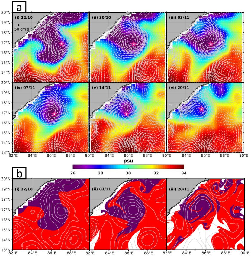
2
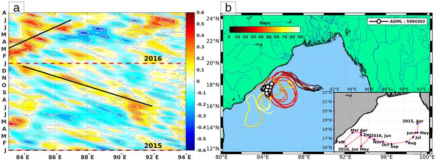
from AVISO. Daily sea surface temperature (SST) is from and dissociated around June 2016 (Figure 1(h),(i)). The west-
the Group of High Resolution Sea Surface Temperature ward (eastward) drift of the eddy early (late) in its life is suc-
(GHRSST) product that is produced at 0.25◦ × 0.25◦ res- cinctly captured by the Hovmöller diagram in Figure S1(a). In
olution, and nighttime SST from Advanced Very High- particular, the speed of translation in these two periods is seen
Resolution Radiometer (AVHRR) instrument of METOP2 to be approximate −6 cm/s and 4 cm/s, respectively. Further,
satellite on a 1.1 km grid. 8-day running mean sea surface while near the western coast, the Rossby number (Ro) — de-
salinity (SSS) estimates are from the Soil Moisture Active fined as ξ/f , where ξ is the relative vorticity of the eddy and
Passive (SMAP) satellite [19] at 60 km resolution, interpo- f is the Coriolis parameter — of this eddy was approximately
lated to a 0.25◦ × 0.25◦ grid. Total surface currents are from 0.2 suggestive of geostrophic balance. Given that the aver-
the Bay of Bengal current and advection estimation (BoBcat), age life span of eddies in the BoB is about two-three months
based on a combination of AVISO geostrophic currents and [9, 11], this particular eddy was remarkable in that it lasted for
directly wind-forced Ekman currents at 1 m depth on a grid about sixteen months. Indeed, such a long life span of eddy
resolution of 0.25◦ × 0.25◦ [4, 53]. Temperature and salin- can be sustained in BoB has not been highlighted so far in the
ity profiles are from Argo floats with 5-day sampling, from literature as far as we are aware.
NOAA’s Atlantic Oceanographic and Meteorological Labora- In the post-monsoon season, the eddy translated along west-
tory [2]. We also use drifter data from the Surface Velocity ern boundary of the Bay and trapped freshwater as shown
Program (SVP), NOAA’s Global Drifter Program [5]. in the SSS maps with surface currents in Figure 2(a). Start-
The ocean reanalysis is the GLORYS12V1 global product that ing in early October, freshwater is pulled inward from the
uses the NEMO ocean model (1/12◦ horizontal resolution, or- western boundary and enters the eddy over a period of about
der 1 m vertical resolution in the upper ocean, 50 vertical lev- 10 days. Coincidentally, five drifters were also trapped and
els) surface forcing from ECMWF ERA-Interim reanalysis, formed loops within the eddy during this period as shown in
covering the satellite altimetry era 1993-2018. Observations Figure S1(b). Signs of chaotic advection [36] of the salinity
are assimilated using a reduced-order Kalman filter, with a field, that are visible via the stretching of the salinity field in
3D-VAR scheme used to correct for the slowly-evolving large- Figure 2(a), are brought out in Figure 2(b) via a tracer experi-
scale biases in temperature and salinity [7, 30]. ment [39], wherein a passive field is initialized with the same
The Lagrangian advection of tracers is performed by BoB- value as the freshwater salinity (SSS≤ 28 psu) on 01/10. The
cat surface currents from a given initial position by integrat- backward finite time Lyapunov exponents (b-FTLEs; see Sup-
ing the surface flow field using a Runge-Kutta fourth-order plementary Material text S1 for definition and computation
method. The velocities are interpolated using a bi-linear in- details) [32, 40] for the BoBcat surface flow are also shown for
terpolation scheme to a grid of resolution 0.01◦ × 0.01◦ . The clarity. As is evident, the freshwater (and tracer) is pulled in
equations involved are described in the supplementary mate- along these attracting manifolds [18, 29] and “fills” the eddy
rial text S1 (Equation 1). Lagrangian measures such as attract- in a span of about 10 days. Thus, in less than two weeks,
ing Lagrangian Coherent Structures (a-LCSs) or backward Fi- the eddy which contained salty water (around 01/10), pulls
nite Time Lyapunov Exponents (b-FTLEs) [25, 35, 68] have in freshwater that forms a layer on its surface (by 21/10). The
also been computed to understand the pathway of freshwater role of mesoscale features in restricting freshwater to the north
trapping further. Details of the calculation of these metrics are Bay has been suggested in other tracer experiments too [3].
provided in the supplementary material (text S1). Given the
timescales of interest here, the backward advection time has
been taken as 20 days to calculate b-FTLEs (a-LCSs). IV. HOMOGENIZATION OF FRESHWATER IN THE
EDDY
III. THE EDDY AND THE ENTRY OF FRESHWATER
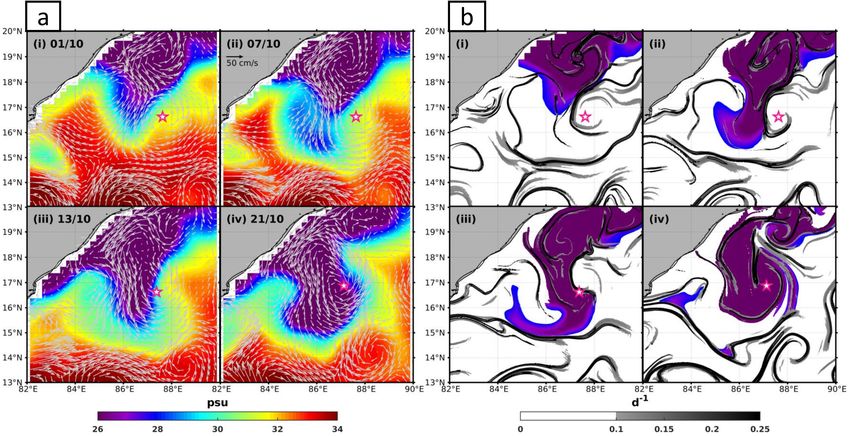
The freshwater that entered the eddy by means of horizontal
chaotic advection remains trapped for more than a month as
Snapshots of the particular eddy for every month that we use seen in the SSS maps in Figure 3(a). Figure 3(b) shows snap-
to highlight interaction with freshwater is shown in Figure shots of the evolution of a passive field (SSS≤28 psu; violet
1. In particular, we show the eddy center (star), sea-level color) within the eddy for this time period. As with SSS, the
anomaly, and geostrophic currents. Consistent with prior passive tracer remains contained in the eddy for the most part,
work [11], this eddy was born at the eastern edge of the though there is a systematic exchange of material across the
Bay. After its genesis (around April 2015), the eddy moved eddy boundary. Specifically, some salty water (SSS>28 psu;
southwest towards the central BoB, then took a northwest- marked by red color) spirals into the eddy while freshwater
ward route from September 2015 onward (Figure 1(a),(b),(c)). (violet) is stretched out in the form of extended filaments that
After the monsoon, the eddy remained close to the western mix into the exterior Bay. For example, the intrusion of red
boundary of BoB. Interestingly, the eddy appeared to decay in filaments that get wrapped into the eddy and violet streaks
size towards the end of 2015 but re-intensified, and its size in- that are stretched out of the eddy can clearly be seen in Figure
creased on the arrival of the northward-flowing EICC [21] dur- 3(b) on 03/11 and 20/11. This exchange of material across
ing spring of 2016 (Figure 1(g)). Finally, the eddy moved east- the “kinematic” boundary of the eddy is a hallmark of chaotic
ward, off of the western boundary, towards the central BoB mixing (see, for example, [27], for a discussion of this mixing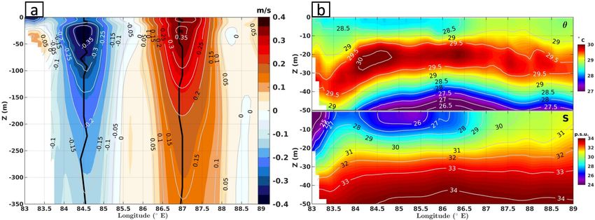
3

FIG. 1: (a)-(i) Mean sea level anomaly (SLA) contours in units of centimeters with geostrophic velocity quivers overlaid on 1st day of the
month for May, July, September, October, November, December 2015, and February, April, June 2016. The contours of SLA are in the range
of -25 cm to 25 cm with 5 cm intervals. The track of the cyclonic eddy is shown with “star” indicating the SLA minimum of the eddy and
“dot” denoting the position in preceding months from its origin.

FIG. 2: (a) Sea Surface Salinity (SSS) with BoBcat current quivers on 01/10, 07/10, 13/10, 21/10, respectively. (b) Advected passive scalar
maps with tracer initialized to SSS< 28 psu on 01/10 for days as in (a). In addition, attracting Lagrangian Coherent Structures (a-LCS) or
b-FTLE computed by integrating backward for 20 days are shown on the top of the tracer field. Only values above 0.1 day−1 (stronger stable
manifolds) are shown.

process and an example from the atmosphere) and is antici-             AOML-5904302 data which was trapped in this eddy from
pated to homogenize salinity inside the eddy. In fact, as can          24/10 to 24/12 (Figure S1(b)). In particular, the evolution of
be seen from the SSS values in Figure 3(a), the freshwater on          potential temperature (θ), salinity (S), potential density (σθ ),
22/10 is much saltier after a month’s time.                            square of the Brunt-Väisälä frequency (N2 = − gρ̄ dρ
                                                                                                                            dz ) where θ,
                                                                                2
The vertical structure of water mass is obtained from Argo             σθ and N has been computed using Gibbs-SeaWater Oceano-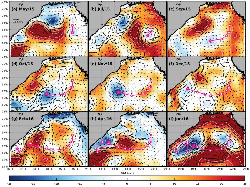
4

FIG. 3: (a)(i)-(vi) shows Sea Surface Salinity (SSS) with BoBcat current quivers on 22/10, 30/10, 03/11, 07/11, 14/11, 20/11, respectively.
Star marks the center of the eddy. (b) Tracers with SSS ≤ 28 (>28) psu initialized on 22/10/2015 are marked in violet (red) colors. These are
advected forward in time by BoBcat currents and shown for 22/10, 03/11, and 20/11 of 2015 with contours of SLA overlaid on the top.

graphic Toolbox [33], and is shown in Figure S2. The ho-                The evolution of mean surface potential temperature (θ), SSS,
mogenization suggested by Figure 3(a) is confirmed via this             sea-level anomaly of the eddy center, and a maximum speed
in situ data by comparing vertical profiles of θ, S and N2 in           of the surface currents over a circle of diameter 300 km across
the early (24/10), middle (18/11) and late (14/12) parts of the         the eddy center is shown in Figure 3b(i),(ii), respectively as it
aforementioned period. Specifically, as per Figure 4(a), on             moves along the western coast of the BoB. Here, we see that
the entry of freshwater (24/10), we clearly see a very shal-            during the entry of freshwater (09/10 till 30/10), SSS drops
low layer (about 5 m) of low salinity water, a small temper-            by 5 approximately psu. Then, consistent with the Argo float
ature inversion, and high buoyancy frequency below the base             data, surface salinity starts increasing. The initial rate of in-
of this fresh layer. This results in a stratified upper layer in        crease is relatively high rate till about 13/11 (approximately 3
the eddy with N2max = 1.07 × 10⁻² s−2 . In a few weeks,                 psu in a week), thereafter, the rate of increase of salinity slows
by 18/11, the surface salinity (temperature) shows signs of in-         down, and by 14/12 the mean eddy salinity is about 30-31 psu.
creasing (decreasing) and the buoyancy frequency has reduced            This indicates that the homogenization of salinity possibly in-
(N2max = 4.1 × 10⁻³ s−2 ). In about a month’s time, i.e., on            volves multiple stages with different mixing rates. Further,
14/12, it becomes clear that surface salinity has increased by          along with this increase in SSS over a month’s time, there is
almost 10 psu in this point measurement and its vertical struc-         systematic surface cooling from about 30.5 to 27.5◦ C and an
ture is weaker. Further, the surface of the eddy has cooled             increase in the sea-level anomaly of the eddy center within the
and there is a marked inversion in temperature at about 25 m            eddy.
[57]. The buoyancy frequency has also reduced significantly             Longitudinal variations across the center of the eddy of sea
(approximately N2max = 1.8 × 10⁻³ s−2 ) and is fairly uniform           level anomaly, θ, and SSS and during pre-freshening (01/10),
with depth. Thus, these profiles of water mass clearly indi-            freshening (31/10), and post freshening days (15/12) are
cate a progressive homogenization of fields and a decrease in           shown in Figure 5. The sea-level anomaly is minimum (about
vertical gradients over the course of a month.
5

FIG. 4: (a)(i),(ii),(iii) shows S (psu), θ (◦ C) and N2 (s−2 ) with depth for upper 60 m on 24/10, 18/11 and 14/12 from Argo AOML-5904302,
respectively. (b) Daily time series of (i) mean θ, SSS (with straight lines to guide the eye) and (ii) maximum current speed and minima of SLA
over a circle of diameter 300 km around the eddy center from 01/10/2015 to 31/12/2015.

FIG. 5: (i), (ii), (iii) shows SLA, θ and SSS cross-sections through the center of the eddy on 01/10, 31/10, and 15/12 representing pre-
freshening, freshening, and post-freshening days, respectively.

−25 cm) and the rate of spinning is at its fastest when fresh-           the progressively lighter blue colors in Figure 6). Given the
est water is in the eddy as compared to pre and post fresh-              relatively higher spatial resolution of NEMO reanalysis, we
ening periods. Consistent with vertical profiles in Figure 5a            can see the exchange of water mass across the kinematic eddy
the potential temperature decreases across the eddy with time            boundary. This is especially clear on 13/11 and 21/11 where
after the entry of freshwater. Interestingly, as seen in Fig-            see freshwater (blue) being pulled out in the south-east corner
ure 5, there is a strong gradient in salinity across the eddy            of the eddy while salty water (red) pushes in on its north-east
of approximately 6 psu in 200 km on 31/10 when freshwater                edge. The three-dimensional nature of reanalysis also allows
filled the eddy. This horizontal gradient relaxes in a month             for a clearer view of the eddy itself — Figure 7(a) shows its
(by 15/12), and not only is the salinity is much higher, but             vertical structure via the meridional velocity (averaged from
sea-level anomalies also become smaller (about −10 cm) and               28/10 to 21/11) up to a depth of 350 m across the section AB
the rate of spinning slows down. Thus, the surface properties            marked in Figure 6(i). The jets supported by this eddy have
and horizontal sections go hand in hand with Argo data and               the highest speeds that are approximately 0.35 m/s at a depth
support the progressive homogenization of freshwater in the              of about 20 m, and most of the eddy signature dies out by 300
eddy.                                                                    m. Through this period of trapping, the reanalysis salinity
                                                                         also shows a freshwater layer restricted to within 10 m from
                                                                         the surface (Figure 7(b); second panel). Further, the inver-
                                                                         sion noted due to surface cooling in the in situ data (Figure
        V.   OCEAN REANALYSIS AND DISCUSSION
                                                                         4(a)) is also captured here at a depth of approximately 25 m
                                                                         as seen in the first panel of Figure 7(b). Thus, in addition to
In the Sections so far, we saw the trapping and homogeniza-              a detailed view of the eddy, while the actual numbers differ
tion of freshwater via in situ and satellite data. Here, we              slightly, the overall picture of the trapping of freshwater and
check if similar features can be detected in the NEMO re-                its progressive homogenization due to lateral mixing is seen
analysis product. Quite clearly, freshwater can be seen inside           in the reanalysis data too.
the eddy over a similar time period (Figure 4a). Further, early          Given the inflow of low salinity water to the Bay every year
on, around 28/10 the water in the eddy is freshest and its salti-        and the ubiquitous presence of eddies on the western coast of
ness progressively increases over the next three weeks (via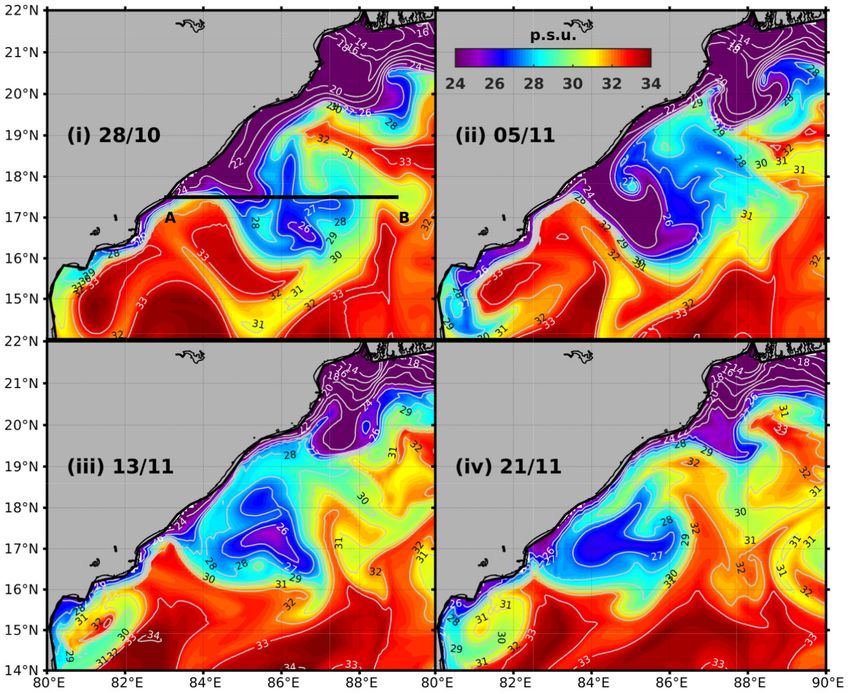
6

the Bay, we suspect that this process of trapping and subse-         into the eddy began in early October. In particular, freshwa-
quent homogenization of surface salinity within an eddy on           ter was directed along with the eddy’s attracting manifolds
the timescale of a month may not be uncommon. The rate of            and bore the hallmarks of chaotic advection. In a time span
homogenization is about 2-3 psu in a week which is compa-            of approximately ten days, the eddy, which contained warm
rable to mixing during strong wind events, for example, trop-        and salty water, had a surface layer of cool freshwater. This
ical cyclone Phailin in 2013 off the west coast of north BoB         led to a strongly stratified surface layer, deep sea-level anoma-
caused a change of about 1-4 psu via wind-induced vertical           lies, high spin rates, and strong lateral gradients in salinity and
mixing [8]. In fact, the increase in SSS by about 5-7 psu in         density across the eddy.
the eddy is of the same order as that noted through the course       The trapped freshwater in the eddy was then observed to be
of the winter season in the northern BoB [1]. Of course, the         progressively homogenized with its environment. Specifi-
outstanding issue that remains is the dynamical cause of mix-        cally, satellite maps showed an increase in salinity in about a
ing in the eddy. Given the strong stratification on the arrival of   month after the freshwater entered the eddy. This was corrob-
fresh water, vertical overturning is likely inhibited [58], even     orated by in situ vertical profiles from Argo data that showed
with the observed surface cooling [31]. While the scale of           an increase in surface salinity along with surface cooling and
the eddy (approx 300 km) is in a balanced regime [55], there         the formation of an inversion layer. Concomitantly, horizontal
are clear indications toward the formation of smaller scales         gradients of salinity and density relaxed over the next month.
from the SSS and SST fields shown in Figure 8(a) and (b).            The homogenization process was illustrated via Lagrangian
For SSS (Figure 8(a)), which is relatively coarse in resolution,     tracer experiments that showed the horizontal mixing that took
salty water can be seen pushing into the eddy on its north-east      place, wherein salty water was advected into the eddy. Fresh-
corner. This is seen in much greater detail with finer scales        water was expelled in thin meandering filaments into the open
along with the cold and warm tongues in the higher resolution        Bay. The trapping, freshwater surface layer, and its homog-
SST map on the same day in Figure 8(b). Indeed, lobe like            enization were also seen in reanalysis data. Thus, in contrast
structures can be seen around the eddy on multiple days dur-         to seasonal timescales where vertical diffusion is important,
ing the homogenization period (Figure 3(a), especially, 30/10,       we have shown that freshwater becomes significantly saltier
03/11, and 07/11). This is reminiscent of the development of         within a month’s timescale, apparently by horizontal mixing
non-axisymmetric features via baroclinic and barotropic insta-       when trapped in a mesoscale eddy.
bility during the adjustment of rotating-stratified shallow vor-
tices that are of a lower density [12, 22, 46, 64] or fresher [56]
than the ambient fluid. These features, especially smaller-
scale vortices within the parent eddy, are also visible in re-                       VII.   ACKNOWLEDGEMENT
analysis data shown in Figure 6 and Figure S3.
Indeed, the large gradients observed on the arrival of fresh-           We thank Dr. Jared Buckley and Prof. Amit Tan-
water are probably even sharper as per ship-based measure-           don for sharing the BoBcat dataset for 2015 (https:
ments in the BoB [42]. At these fine scales of O(1-10 km)            //github.com/jbuckley-BoBcat/BoBcat).                        NP
frictional as well as diabatic surface fluxes can play an im-        would like to acknowledge Dr.             J Sree Lekha and
portant role in potential vorticity extraction or injection to       Dr. Dipanjan Chaudhuri for discussions. The authors
generate instability and subsequent sub-mesoscale turbulence         would like to acknowledge the following data sources:
[15, 42, 45, 59, 60]. In effect, we suspect that the SST in          National Oceanic and Atmospheric Administration’s At-
Figure 8(b) just provides a glimpse into the horizontal mixing       lantic Oceanographic and Meteorological Laboratory, Physi-
and turbulence triggered by the adjustment process in such           cal Oceanography Division (https://www.aoml.noaa.
freshwater eddies and motivates further study based on situ          gov/phod/gdp/) for distributing Argo and Drifter data;
observations along with high resolution modeling to under-           Copernicus Marine and Environment Monitoring Service
stand the mechanism behind the homogenization of salinity at         (CMEMS) for Ssalto Duacs/gridded multimission altime-
sub-mesoscales.                                                      ter products from AVISO and GLORYS12V1 product
                                                                     driven by the NEMO model (https://resources.
                                                                     marine.copernicus.eu/); Physical Oceanography Ac-
                     VI.   CONCLUSIONS
                                                                     tive Archive Centre for distributing SMAP (Soil Moisture
                                                                     Active Passive) satellite sea surface salinity data (https:
                                                                     //doi.org/10.5067/SMP43-3TPCS) and Group for
By using satellite, in situ and reanalysis data, we have shown       High Resolution Sea Surface Temperature (GHRSST) data
that freshwater discharged into the Bay of Bengal was trapped        (https://podaac.jpl.nasa.gov/GHRSST/). We
in a cyclonic mesoscale eddy during the postmonsoon season           also thank the Divecha Centre for Climate Change, IISc, Ban-
of 2015. The eddy responsible for trapping freshwater was            galore, for providing financial assistance. JS would like to ac-
itself unique in that it lasted for almost sixteen months in the     knowledge support from the University Grants Commission
Bay, where the usual lifetimes of eddies are of the order of         (UGC) for funding via 6-3/2018 under the 4th cycle of the
two months. During its lifetime, the eddy remained close to          Indo-Israel joint research program. DS acknowledges support
the Bay’s western coast for almost three months in the post-         from the National Monsoon Mission, IITM, Pune. NP and JS
monsoon season. In this period, entry of low salinity water          would like to thank Pattabhi Rama Rao E, Dr. N. Srinivasa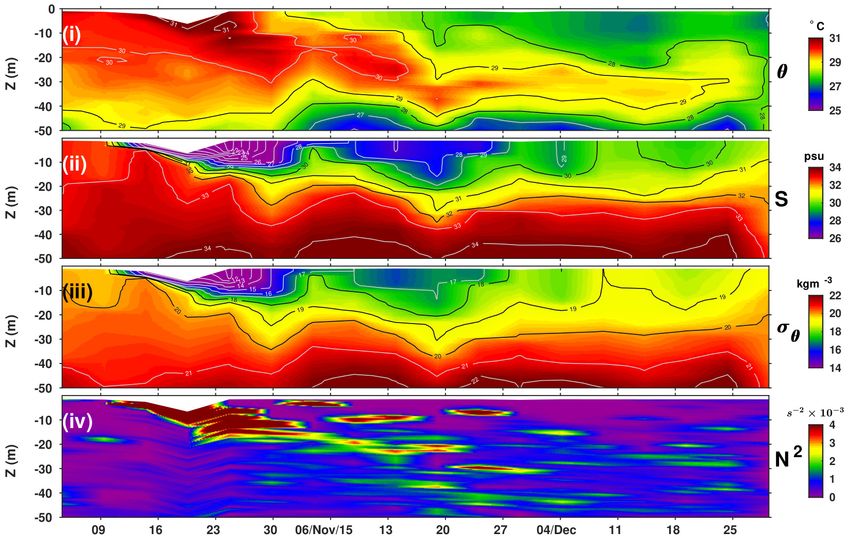
7

FIG. 6: (i)-(iv) SSS (psu) (with contours) at 0.5 m from NEMO reanalysis from 28/10 to 21/11 (freshwater trapping days) with 8-day interval.
AB denotes the cross-section of the eddy from 83◦ E-89◦ E shown in subpanel (i).

FIG. 7: (a) Mean meridional velocity profile along the longitudinal section AB of the eddy up to a depth of 350 m shown in Figure 6(i)
averaged over freshwater trapping days (28/10–21/11) from NEMO reanalysis data. The vertical black lines indicate the contours of maximum
speed on each side of the lobes of the eddy. (b) Variation of mean potential temperature (θ) (upper panel) and mean salinity (lower panel)
within upper 50 m of the eddy averaged for the same section and time period as in (a).

Rao and Geetha Gujjari of ESSO - Indian National Centre                      VIII. SUPPORTING INFORMATION FOR “EDDY
for Ocean Information Services (https://incois.gov.                         INDUCED TRAPPING AND HOMOGENIZATION OF
in/), Ministry of Earth Sciences, Government of India for                        FRESHWATER IN THE BAY OF BENGAL”
sharing the METOP2-AVHRR SST data.
                                                                                                   A.   SI: Text

                                                                        Attracting Lagrangian Coherent Structures (a-LCSs or
                                                                        Backward Finite Time Lyapunov Exponents (b-FTLEs):
                                                                        The mixing of freshwater is characterized from a Lagrangian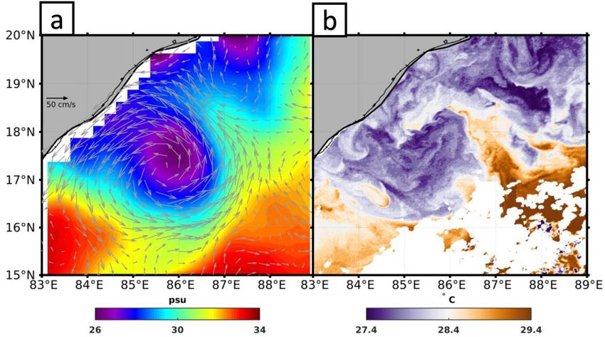
8

                            FIG. 8: (a) SSS (psu) with BoBcat currents (b) METOP2-AVHRR SST (◦ C) on 13/11/2015.

perspective via so-called backward Finite Time Lyapunov Ex-                        The gradient of the flow map ∇Ftt0 (x0 ) is computed using
ponents (b-FTLEs) [68]. These are ridges that represent at-                        an auxiliary grid about the reference point [35], and can be
tracting Lagrangian coherent structures in a flow [24]. To                         written as,
compute the b-FTLEs, we first advect fluid parcel by integrat-
ing the following equations backward in time,

                                                                                                                             α11 α12
                                                                                                       ∇Ftt0 (x0 )   ≈                 ,                  (4)
                                                                                                                             α21 α22
                dφ   u(φ, λ, t) dλ   v(φ, λ, t)
                   =           ,   =            .                           (1)
                dt   R cos(λ) dt        R                                          where,
Here, φ, λ, u and v are the latitude, longitude, zonal and
meridional velocity, respectively. R is the radius of the earth.                                   xi (t; t0 , x0 + δxj ) − xi (t; t0 , x0 − δxj )
The time span is t = t0 to t = to −τ and the numerical method                             αi,j ≡                                                   .      (5)
                                                                                                                      2|δxj |
employed is the 4th order Runge-Kutta scheme. The velocity
data (u, v) is given on a fixed grid and the flow has been inter-                  Finally, the largest b-FTLE [24, 25, 32] associated with the
polated by a bilinear interpolation scheme. We then compute                        trajectory x(t, t0 , x0 ) over the time interval [t0 , t] is defined
the right Cauchy-Green Lagrange tensor Ctt0 associated with                        as,
the flow map Ftt0 (x0 ), which is defined as,

                                                                                                                1          q
                                               T
               Ctt0 (x0 ) = (∇Ftt0 (x0 )) ∇Ftt0 (x0 ).                      (2)              λτ (x0 ) = −              log( λmax [Ctt0 (x0 )]).           (6)
                                                                                                             |t − t0 |
Ftt0 (x0 ) denotes the position of a parcel at time t backward
                                                                                   The backward integration time |τ | = |t−t0 | has been taken as
in time, advected by the flow from an initial time and posi-
                                                                                   20 days and computed on a finer grid resolution 0.01◦ ×0.01◦ .
tion (t0 , x0 ). Ctt0 (x0 ) is symmetric and positive definite, its
eigenvalues (λ0 s) and eigenvectors (ξ 0 s) can be written as,

                                                                                                        B.    SI: Figure (S1, S2, S3)
             Ctt0 (x0 ) = λi ξi , 0 < λ1 ≤ λ2 , i = 1, 2.                   (3)

 [1] V. Akhil, F. Durand, M. Lengaigne, J. Vialard, M. Keerthi, V. V.                   (Argo GDAC). SEANOE, 2000. doi: 10.17882/42182.
     Gopalakrishna, C. Deltel, F. Papa, and C. de Boyer Montégut. A model-         [3] R. Benshila, F. Durand, S. Masson, R. Bourdallé-Badie,
     ing study of the processes of surface salinity seasonal cycle in the Bay of        C. de Boyer Montégut, F. Papa, and G. Madec. The upper Bay
     Bengal. Journal of Geophysical Research: Oceans, 119(6):3926–3947,                 of Bengal salinity structure in a high-resolution model.        Ocean
     2014. doi: 10.1002/2013JC009632.                                                   Modelling, 74:36–52, 2014. doi: 10.1016/j.ocemod.2013.12.001.
 [2] Argo. Argo float data and metadata from global data assembly centre            [4] J. M. Buckley, B. Mingels, and A. Tandon. The impact of lateral advec-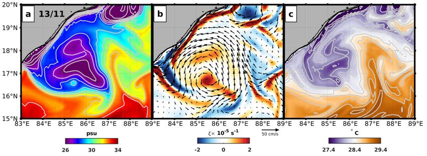
9

FIG. S1: (a) Hovmöller diagram of Rossby number (ξ/f ) computed from geostrophic currents averaged over 16.625◦ N-17.625◦ N shown for
the year 2015-2016. (b) Track of Argo float (AOML-5904302) and trajectories of Surface Velocity Program (SVP) “drifters” (drouged at 15
m depth) within the eddy from 01/10 to 31/12 of 2015 and entire track of eddy in inset from the first day of April 2015 to June 2016 in an
interval of a month.

FIG. S2: (i) Potential temperature (θ), (ii) salinity (S), (iii) potential density (σθ ) and (iv) squared Brunt-väisälä frequency (N2 ), respectively
with depth using Argo AOML-5904302 data for the upper 50 m from October to December, 2015.

     tion on SST and SSS in the northern Bay of Bengal during 2015. Deep                operational oceanography. GODAE OceanView, 2018. doi: 10.17125/
     Sea Research Part II: Topical Studies in Oceanography, 172:104653,                 gov2018.
     2020. doi: 10.1016/j.dsr2.2019.104653.                                       [8]   D. Chaudhuri, D. Sengupta, E. D’Asaro, R. Venkatesan, and
 [5] L. R. Centurioni, J. D. Turton, R. Lumpkin, L. Braasch, G. Brassington,            M. Ravichandran. Response of the salinity-stratified Bay of Bengal to
     Y. Chao, E. Charpentier, Z. Chen, G. Corlett, K. Dohan, et al. Global              cyclone Phailin. Journal of Physical Oceanography, 49(5):1121–1140,
     in-situ observations of essential climate and ocean variables at the air-          2019. doi: 10.1175/JPO-D-18-0051.1.
     sea interface. Frontiers in Marine Science, 6:419, 2019. doi: 10.3389/       [9]   G. Chen, D. Wang, and Y. Hou. The features and interannual variability
     fmars.2019.00419.                                                                  mechanism of mesoscale eddies in the Bay of Bengal. Continental Shelf
 [6] A. Chaitanya, M. Lengaigne, J. Vialard, V. Gopalakrishna, F. Durand,               Research, 47:178–185, 2012. doi: 10.1016/j.csr.2012.07.011.
     C. Kranthikumar, C. Amritash, V. Suneel, F. Papa, and M. Ravichan-          [10]   X. Cheng, S.-P. Xie, J. P. McCreary, Y. Qi, and Y. Du. Intraseasonal vari-
     dran. Salinity Measurements Collected by Fishermen Reveal a “River                 ability of sea surface height in the Bay of Bengal. Journal of Geophysi-
     in the Sea” Flowing Along the Eastern Coast of India. BAMS, pages                  cal Research: Oceans, 118(2):816–830, 2013. doi: 10.1002/jgrc.20075.
     1897–1908, 2014. doi: 10.1175/BAMS-D-12-00243.1.                            [11]   X. Cheng, J. P. McCreary, B. Qiu, Y. Qi, Y. Du, and X. Chen. Dy-
 [7] E. Chassignet, A. Pascual, J. Tintoré, and J. Verron. New frontiers in            namics of eddy generation in the central Bay of Bengal. Journal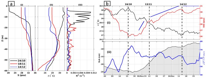
10

FIG. S3: (a) SSS with contours with an interval of 1 psu (b) vorticity with surface current quiver (c) SST with contours with an interval of
0.2◦ C at 0.5 m depth on 13/11/2015 from NEMO reanalysis data.

       of Geophysical Research: Oceans, 123(9):6861–6875, 2018. doi:                 [24] G. Haller. Lagrangian coherent structures from approximate veloc-
       10.1029/2018JC014100.                                                              ity data. Physics of Fluids, 14(6):1851–1861, 2002. doi: 10.1063/1.
[12]   F. Chia, R. Griffiths, and P. Linden. Laboratory experiments on fronts:            1477449.
       part II: the formation of cyclonic eddies at upwelling fronts. Geophys-       [25] G. Haller and T. Sapsis. Lagrangian coherent structures and the smallest
       ical & Astrophysical Fluid Dynamics, 19(3-4):189–206, 1982. doi:                   finite-time Lyapunov exponent. Chaos: An Interdisciplinary Journal of
       10.1080/03091928208208955.                                                         Nonlinear Science, 21(2):023115, 2011. doi: 10.1063/1.3579597.
[13]   A. Dai and K. E. Trenberth. Estimates of freshwater discharge from            [26] S. Howden and R. Murtugudde. Effects of rives inputs into the Bay
       continents: Latitudinal and seasonal variations. Journal of hydrometeo-            of Bengal. Journal of Geophysical Research, 106(C9):19825–19843,
       rology, 3(6):660–687, 2002. doi: 10.1175/1525-7541(2002)003h0660:                  2001. doi: 10.1029/2000JC000656.
       EOFDFCi2.0.CO;2.                                                              [27] B. Joseph and B. Legras. Relation between Kinematic Boundaries, Stir-
[14]   S. Dandapat and A. Chakraborty. Mesoscale eddies in the Western Bay                ring, and Barriers for the Antarctic Polar Vortex. Journal of the Atmo-
       of Bengal as observed from satellite altimetry in 1993–2014: statisti-             spheric Sciences, 59:1198–1212, 2002. doi: 10.1175/1520-0469(2002)
       cal characteristics, variability and three-dimensional properties. IEEE            059h1198:RBKBSAi2.0.CO;2.
       Journal of Selected Topics in Applied Earth Observations and Remote           [28] P. V. H. Kumar, B. Mathew, M. R. R. Kumar, A. R. Rao, P. S. V. Ja-
       Sensing, 9(11):5044–5054, 2016.                                                    gadeesh, K. G. Radhakrishnan, and T. N. Shyni. ‘Thermohaline front’
[15]   E. D’Asaro, C. Lee, L. Rainville, R. Harcourt, and L. Thomas. Enhanced             off the east coast of India and its generating mechanism. Ocean Dynam-
       turbulence and energy dissipation at ocean fronts. Science, 332(6027):             ics, 63:1175–1180, 2013. doi: 10.1007/s102360130652y.
       318–322, 2011. doi: 10.1126/science.1201515.                                  [29] Y. Lehahn, F. d’Ovidio, M. Lévy, and E. Heifetz. Stirring of the north-
[16]   T. Delcroix, A. Chaigneau, D. Soviadan, J. Boutin, and C. Pegliasco.               east Atlantic spring bloom: A Lagrangian analysis based on multisatel-
       Eddy-Induced Salinity Changes in the Tropical Pacific. Journal of Geo-             lite data. Journal of Geophysical Research: Oceans, 112(C8), 2007.
       physical Research: Oceans, 124(12):374–389, 2019. doi: 10.1029/                    doi: 10.1029/2006JC003927.
       2018JC014394.                                                                 [30] J.-M. Lellouche, E. Greiner, O. Le Galloudec, G. Garric, C. Reg-
[17]   C. Dong, J. C. McWilliams, Y. Liu, and D. Chen. Global heat and salt               nier, M. Drevillon, M. Benkiran, C.-E. Testut, R. Bourdalle-Badie,
       transports by eddy movement. Nature communications, 5(1):1–6, 2014.                F. Gasparin, et al. Recent updates to the Copernicus Marine Ser-
[18]   F. d’Ovidio, V. Fernández, E. Hernández-Garcı́a, and C. López. Mix-             vice global ocean monitoring and forecasting real-time 1/12◦ high-
       ing structures in the Mediterranean Sea from finite-size Lyapunov ex-              resolution system. Ocean Science, 14(5):1093–1126, 2018. doi:
       ponents. Geophysical Research Letters, 31(17), 2004. doi: 10.1029/                 10.5194/os-14-1093-2018.
       2004GL020328.                                                                 [31] A. Mahadevan, G. Spiro Jaeger, M. Freilich, M. Omand, E. Shroyer,
[19]   A. G. Fore, S. H. Yueh, W. Tang, B. W. Stiles, and A. K. Hayashi.                  and D. Sengupta. Freshwater in the Bay of Bengal: Its fate and role in
       Combined active/passive retrievals of ocean vector wind and sea surface            air-sea heat exchange. Oceanography, 29:72–81, 2016. doi: 10.5670/
       salinity with SMAP. IEEE Transactions on Geoscience and Remote                     oceanog.2016.40.
       Sensing, 54(12):7396–7404, 2016. doi: 10.1109/TGRS.2016.2601486.              [32] M. Mathur, M. J. David, R. Sharma, and N. Agarwal. Thermal
[20]   S. Fournier, J. Vialard, M. Lengaigne, T. Lee, M. M. Gierach, and                  fronts and attracting Lagrangian Coherent Structures in the north Bay
       A. V. S. Chaitanya. Modulation of the Ganges-Brahmaputra river plume               of Bengal during December 2015–March 2016. Deep Sea Research
       by the Indian Ocean dipole and eddies inferred from satellite observa-             Part II: Topical Studies in Oceanography, 168:104636, 2019. doi:
       tions. Journal of Geophysical Research: Oceans, 122(12):9591–9604,                 10.1016/j.dsr2.2019.104636.
       2017. doi: 10.1002/2017JC013333.                                              [33] T. J. McDougall and P. M. Barker. Getting started with TEOS-10 and
[21]   A. Gangopadhyay, G. Bharat Raj, A. H. Chaudhuri, M. Babu, and                      the Gibbs Seawater (GSW) oceanographic toolbox. SCOR/IAPSO WG,
       D. Sengupta. On the nature of meandering of the springtime western                 127:1–28, 2011.
       boundary current in the Bay of Bengal. Geophysical Research Letters,          [34] S. Neetu et al. Premonsoon/Postmonsoon Bay of Bengal tropical cy-
       40(10):2188–2193, 2013. doi: 10.1002/grl.50412.                                    clones intensity: role of Air-Sea coupling and large-scale background
[22]   R. Griffiths and P. Linden. The stability of vortices in a rotating, strat-        state. Geophysical Research Letters, 46:2149–2157, 2019. doi: 10.
       ified fluid. Journal of Fluid Mechanics, 105:283–316, 1981. doi:                   1029/2018GL081132.
       10.1017/S0022112081003212.                                                    [35] K. Onu, F. Huhn, and G. Haller. LCS Tool: A computational platform
[23]   G. Grunseich, B. Subrahmanyam, and B. Wang. The Madden-Julian                      for Lagrangian coherent structures. Journal of Computational Science,
       oscillation detected in Aquarius salinity observations. Geophysical Re-            7:26–36, 2015. doi: 10.1016/j.jocs.2014.12.002.
       search Letters, 40, 2013. doi: 10.1002/2013GL058173.                          [36] J. Ottino. The kinematics of mixing: stretching, chaos, and transport,
11
volume 3. Cambridge university press, 1989. cillations in SMAP salinity in the Bay of Bengal. Geophysical Research
[37] F. Papa, S. K. Bala, R. K. Pandey, F. Durand, V. Gopalakrishna, A. Rah- Letters, 45(14):7057–7065, 2018. doi: 10.1029/2018GL078662.
man, and W. B. Rossow. Ganga-Brahmaputra river discharge from [55] J. Sukhatme, D. Chaudhuri, J. MacKinnon, S. Shivaprasad, and D. Sen-
Jason-2 radar altimetry: an update to the long-term satellite-derived gupta. Near-surface ocean kinetic energy spectra and small scale inter-
estimates of continental freshwater forcing flux into the Bay of Ben- mittency from ship based ADCP data in the Bay of Bengal. Journal of
gal. Journal of Geophysical Research: Oceans, 117(C11), 2012. doi: Physical Oceanography, 2020. doi: 10.1175/JPO-D-20-0065.1.
10.1029/2012JC008158. [56] B. Tartinville, E. Deleersnijder, P. Lazure, R. Proctor, K. Ruddick, and
[38] S. Parampil, A. Gera, M. Ravichandran, and D. Sengupta. Intraseasonal R. Uittenbogaard. A coastal ocean model intercomparison study for a
response of mixed layer temperature and salinity in the Bay of Bengal three-dimensional idealised test case. Applied mathematical modelling,
to heat and freshwater flux. Journal of Geophysical Research: Oceans, 22(3):165–182, 1998. doi: 10.1016/S0307-904X(98)00015-8.
115, 2010. doi: 10.1029/2009JC005790. [57] P. Thadathil, V. Gopalakrishna, P. Muraleedharan, G. Reddy, N. Araligi-
[39] N. Paul and J. Sukhatme. Seasonality of surface stirring by geostrophic dad, and S. Shenoy. Surface layer temperature inversion in the Bay of
flows in the Bay of Bengal. Deep Sea Research Part II: Topical Studies Bengal. Deep Sea Research Part I: Oceanographic Research Papers, 49
in Oceanography, 172:104684, 2020. doi: 10.1016/j.dsr2.2019.104684. (10):1801–1818, 2002. doi: 10.1016/S0967-0637(02)00044-4.
[40] V. Pérez-Munuzuri. Mixing and clustering in compressible chaotic [58] R. Thakur, E. L. Shroyer, R. Govindarajan, J. T. Farrar, R. A. Weller,
stirred flows. Physical Review E, 89(2):022917, 2014. doi: 10.1103/ and J. N. Moum. Seasonality and Buoyancy Suppression of Turbulence
PhysRevE.89.022917. in the Bay of Bengal. Geophysical Research Letters, 46(8):4346–4355,
[41] J. T. Potemra, M. E. Luther, and J. J. O’Brien. The seasonal circulation 2019. doi: 10.1029/2018GL081577.
of the upper ocean in the Bay of Bengal. Journal of Geophysical Re- [59] L. N. Thomas. Destruction of potential vorticity by winds. Journal
search: Oceans, 96(C7):12667–12683, 1991. doi: 10.1029/91JC01045. of physical oceanography, 35(12):2457–2466, 2005. doi: 10.1175/
[42] S. Ramachandran, A. Tandon, J. Mackinnon, A. J. Lucas, R. Pinkel, JPO2830.1.
A. F. Waterhouse, J. Nash, E. Shroyer, A. Mahadevan, R. A. Weller, [60] L. N. Thomas, J. R. Taylor, E. A. D’Asaro, C. M. Lee, J. M. Klymak,
et al. Submesoscale processes at shallow salinity fronts in the Bay of and A. Shcherbina. Symmetric instability, inertial oscillations, and tur-
Bengal: Observations during the winter monsoon. Journal of Physical bulence at the Gulf Stream front. Journal of Physical Oceanography,
Oceanography, 48(3):479–509, 2018. doi: 10.1175/JPO-D-16-0283.1. 46(1):197–217, 2016. doi: 10.1175/JPO-D-15-0008.1.
[43] R. Rao and R. Sivakumar. Seasonal variability of sea surface salinity [61] C. Trott and B. Subrahmanyam. Detection of intraseasonal oscillations
and salt budget of the mixed layer of the north Indian Ocean. Journal of in the Bay of Bengal using altimetry. Atmospheric Science Letters, 20
Geophysical Research, 108:3009, 2003. doi: 10.1029/2001JC000907. (7):e920, 2019. doi: 10.1002/asl.920.
[44] D. Samanta, S. N. Hameed, D. Jin, V. Thilakan, M. Ganai, S. A. Rao, [62] C. Trott, B. Subrahmanyam, H. Roman-Stork, V. Murty, and
and M. Deshpande. Impact of a narrow coastal Bay of Bengal sea sur- C. Gnanaseelan. Variability of Intraseasonal Oscillations and Synop-
face temperature front on an Indian summer monsoon simulation. Sci- tic Signals in Sea Surface Salinity in the Bay of Bengal. Journal of
entific reports, 8(1):1–12, 2018. doi: 10.1038/s41598-018-35735-3. Climate, 32, 2019. doi: 10.1175/JCLI-D-19-0178.1.
[45] S. Sarkar, H. T. Pham, S. Ramachandran, J. D. Nash, A. Tandon, [63] C. Trott et al. Eddy-Induced Temperature and Salinity Variability in the
J. Buckley, A. A. Lotliker, and M. M. Omand. The interplay be- Arabian Sea. Geophysical Research Letters, 46:2734–2742, 2019. doi:
tween submesoscale instabilities and turbulence in the surface layer 10.1029/2018GL081605.
of the Bay of Bengal. Oceanography, 29(2):146–157, 2016. doi: [64] R. Verzicco, F. Lalli, and E. Campana. Dynamics of baroclinic vortices
10.5670/oceanog.2016.47. in a rotating, stratified fluid: a numerical study. Physics of Fluids, 9(2):
[46] P. M. Saunders. The instability of a baroclinic vortex. Journal of Phys- 419–432, 1997. doi: 10.1063/1.869136.
ical Oceanography, 3(1):61–65, 1973. doi: 10.1175/1520-0485(1973) [65] P. Vinayachandran and J. Kurian. Hydrographic observations and model
003h0061:TIOABVi2.0.CO;2. simulation of the Bay of Bengal freshwater plume. Deep Sea Research,
[47] F. A. Schott and J. P. McCreary Jr. The monsoon circulation of the Part I, 51:471–486, 2007. doi: 10.1016/dsr.2007.01.007.
Indian Ocean. Progress in Oceanography, 51(1):1–123, 2001. doi: [66] P. Vinayachandran and R. Nanjundiah. Indian Ocean sea surface salinity
10.1016/S0079-6611(01)00083-0. variations in a coupled model. Climate Dynamics, 33:245–263, 2009.
[48] D. Sengupta, G. Bharath Raj, M. Ravichandran, J. Sree Lekha, and doi: 10.1007/s0038200805116.
F. Papa. Near-surface salinity and stratification in the north Bay of Ben- [67] P. Vinayachandran, T. Kagimoto, Y. Masumoto, P. Chauhan, S. Nayak,
gal from moored observations. Geophysical Research Letters, 43(9): and T. Yamagata. Bifurcation of the East India Coastal Current east
4448–4456, 2016. doi: 10.1002/2016GL068339. of Sri Lanka. Geophysical Research Letters, 32, 2005. doi: 10.1029/
[49] H. Seo, S.-P. Xie, R. Murtugudde, M. Jochum, and A. J. Miller. Seasonal 2005GL022864.
effects of Indian Ocean freshwater forcing in a regional coupled model. [68] S. Wiggins. The dynamical systems approach to Lagrangian transport
Journal of Climate, 22:6577–6596, 2009. doi: 10.1175/2009JCLI2990. in oceanic flows. Annu. Rev. Fluid Mech., 37:295–328, 2005. doi: 10.
1. 1146/annurev.fluid.37.061903.175815.
[50] D. Shankar, P. Vinayachandran, and A. Unnikrishnan. The monsoon
currents in the north Indian Ocean. Progress in oceanography, 52(1):
63–120, 2002. doi: 10.1016/S0079-6611(02)00024-1.
[51] S. Shenoi, D. Shankar, and S. Shetye. Difference in heat budgets of the
near-surface Arabian Sea and Bay of Bengal: Implications for the sum-
mer monsoon. Journal of Geophysical Research, 107:283–316, 2002.
doi: 10.1029/2000JC000679.
[52] S. Shetye, A. Gouveia, D. Shankar, S. Shenoi, P. Vinayachandran,
D. Sundar, G. Michael, and G. Nampoothiri. Hydrography and circula-
tion in the western Bay of Bengal during the northeast monsoon. Journal
of Geophysical Research: Oceans, 101(C6):14011–14025, 1996. doi:
10.1029/95JC03307.
[53] J. Sree Lekha, J. Buckley, A. Tandon, and D. Sengupta. Subseasonal
dispersal of freshwater in the northern Bay of Bengal in the 2013 sum-
mer monsoon season. Journal of Geophysical Research: Oceans, 123
(9):6330–6348, 2018. doi: 10.1029/2018JC014181.
[54] B. Subrahmanyam, T. CB, and V. Murty. Detection of intraseasonal os-You can also read