Laplacian Support Vector Machine for Vibration-Based Robotic Terrain Classification - MDPI
←
→
Page content transcription
If your browser does not render page correctly, please read the page content below

electronics
Article
Laplacian Support Vector Machine for
Vibration-Based Robotic Terrain Classification
Wenlei Shi 1 , Zerui Li 2 , Wenjun Lv 2,∗ , Yuping Wu 3 , Ji Chang 2 and Xiaochuan Li 4
 1    School of Economics and Management, Beijing University of Technology, Beijing 100124, China;
      shiwenlei@emails.bjut.edu.cn
 2    Department of Automation, University of Science and Technology of China, Hefei 230027, China;
      lzerui@mail.ustc.edu.cn (Z.L.); cjchange@mail.ustc.edu.cn (J.C.)
 3    School of Electrical Engineering, Yanshan University, Qinhuangdao 066004, China; ypwu@zjut.edu.cn
 4    Faculty of Technology, De Montfort University, Leicester LE1 9BH, UK; xiaochuan.li@dmu.ac.uk
 *    Correspondence: lvwenjun@mail.ustc.edu.cn

 Received: 19 February 2020; Accepted: 17 March 2020; Published: 20 March 2020

 Abstract: The achievement of robot autonomy has environmental perception as a prerequisite.
 The hazards rendered from uneven, soft and slippery terrains, which are generally named
 non-geometric hazards, are another potential threat reducing the traversing efficient, and therefore
 receiving more and more attention from the robotics community. In the paper, the vibration-based
 terrain classification (VTC) is investigated by taking a very practical issue, i.e., lack of labels, into
 consideration. According to the intrinsic temporal correlation existing in the sampled terrain sequence,
 a modified Laplacian SVM is proposed to utilise the unlabelled data to improve the classification
 performance. To the best of our knowledge, this is the first paper studying semi-supervised learning
 problem in robotic terrain classification. The experiment demonstrates that: (1) supervised learning
 (SVM) achieves a relatively low classification accuracy if given insufficient labels; (2) feature-space
 homogeneity based semi-supervised learning (traditional Laplacian SVM) cannot improve supervised
 learning’s accuracy, and even makes it worse; (3) feature- and temporal-space based semi-supervised
 learning (modified Laplacian SVM), which is proposed in the paper, could increase the classification
 accuracy very significantly.

 Keywords: non-geometric hazards; terrain classification; vibration; semi-supervised learning

1. Introduction
     Achieving autonomous motion of a mobile robot is one of the most challenging problems in
robotics, and the key to its success consists of the following four parts: environmental perception, pose
estimation, motion control and route planning [1]. The implementation of pose estimation, motion
control and route planning often requires us to introduce environmental information to some extent,
so accurate environmental perception is of great importance [2]. The environmental humps (e.g.,
walls) and sinks (e.g., rivers) that robots cannot traverse are referred to as geometric hazards, which
have been investigated extensively [3]. On the other hand, the hazards rendered from the uneven,
soft and slippery terrains, which are often called non-geometric hazards, are receiving more and more
attention from the robotics community [4].Different from geometric hazards, non-geometric hazards
do not obstruct the traversing robot completely, but have a great impact on the traversing efficiency [5].
Inappropriately planned routes and an improper control strategy may lead the robot to waste too much
energy, or even cause a loss in mobility. Therefore, if the robot can predict its current and forward
terrain type accurately and in real time, then it can replan its route in time to avoid non-geometric
hazards. Apart from its great effect on route planing, robotic terrain classification also contributes to

Electronics 2020, 9, 513; doi:10.3390/electronics9030513                    www.mdpi.com/journal/electronics
Electronics 2020, 9, 513                                                                             2 of 19

other functions. Because the robotic kinematics/dynamics models contain some parameters which are
determined by the type of the traversing terrain, accurate and real-time terrain classification could
improve the performances of pose estimation [6], motion control [7], energy consumption prediction [8],
etc. [9–11].
      The terrain type is commonly defined by a human according to its appearance, so robotic vision
can be a direct and effective approach to classifying the terrain traversed, being traversed, or to be
traversed. That method is named visual terrain classification; it has been investigated intensively.
In [12], the traditional texture descriptors and non-traditional descriptors, such as Speeded Up Robust
Features (SURF), Fast Local Descriptor for Dense Matching (DAISY) and Contrast Context Histogram
(CCH), are employed to extract visual features, and the random forest is used to distinguish five
different common terrains. In their further work, the results show that the performance of SURF and
DAISY outdoes the traditional texture descriptors in processing terrain images in high resolution [13].
In [14], the visual terrain classification using SURF and random forest as the feature extractor is
studied for outdoor flying robots. The combination of a bag of visual words created from SURF and
the SVM classifier is proposed to discriminate six types of terrains [15]. In their work, a gradient
descent inspired algorithm and the sliding window technique are used to improve its classification
performance. As in [15], the bag of visual words framework is also used in [16]. However, they do not
only consider the effect of feature extraction on visual terrain classification, but also study the other
steps, including codebook generation, feature coding, pooling and normalisation, in the framework.
Several feature fusion methods are studied as well [16]. Comparative study of different features
(including Color and Edge Directivity Descriptor (CEDD), Fuzzy Color and Texture Histogram (FCTH)
and Joint Composite Descriptor (JCD)) and classifiers (including Extreme Learning Machine (ELM),
Support Vector Machine (SVM) and Neural Network (NN)) applying it to visual terrain classification is
presented in [17].Experiment results demonstrate that the combination of JCD and ELM has the highest
generalisation performance. In [18], downward and forward-looking cameras are both employed to
recognise the terrain being traversed and that to be traversed, respectively. The downward-looking
terrain images are used to improve the prediction of the coming terrain. More work concerning terrain
classification using robotic vision can be seen in [19–21].
      The vision provides a mass of colour and texture characteristics, so the visual terrain classification
performs well in an environment with appropriate illumination [22]. When environmental illumination
is unstable or becomes extremely strong or weak, the classification results may be exceedingly
unreliable [4]. Since vision-based terrain classification is non-contacting and exteroceptive, it is
susceptible to the interference of the external environment. In fact, we can employ proprioceptive
sensors to measure the robot–terrain interaction, e.g., haptics and vibration, to realise terrain
classification [23]. The haptic terrain classification was first proposed in 2010 [24]. In the paper,
the current of leg joint motor and the haptic force are used to estimate terrain properties, thereby
increasing the kinematic stability. The features are extracted in the time domain directly and fed into a
multi-class AdaBoost classifier; and finally, the classifier could recognise four different terrains with an
accuracy of 94%. Furthermore, because the errors of a joint gait loop are easy to be measured by the
position sensors which have been built in motors, they can be used to classify different terrains, as a
replacement of ground contact force [25]. Similar work can be found in [26–29]. Because haptic sensors
are generally mounted on the bottoms of robotic feet, the haptic terrain classification is only applicable
to legged mobile robots rather than wheeled ones. For wheeled mobile robots, vibration-based terrain
classification is a promising proprioceptive method for predicting terrains, the data of which could be
easily gathered by an accelerometer mounted on the robot chassis.
      Karl Iagnemma’s team at Massachusetts institute of technology, which was involved in the Mars
mission, is responsible for the environmental perception of the Martian terrains, and first proposed
the terrain classification by means of the analysis of the vibration signals generated by robot–terrain
interaction [30]. Vibration-based terrain classification is more immune to lighting variation than that
based on vision. In [31], a support vector machine is applied to classify six different terrains with an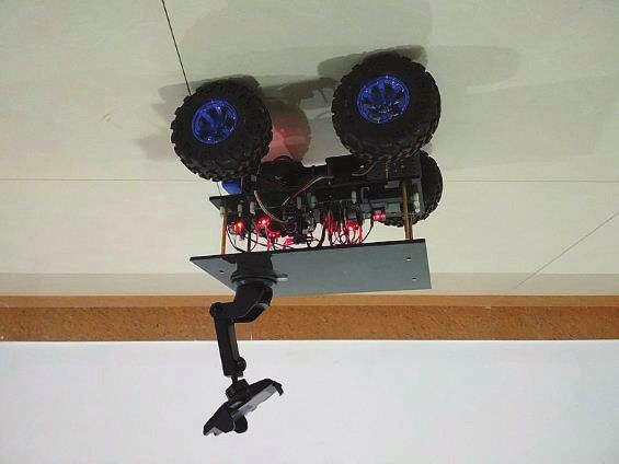
Electronics 2020, 9, 513                                                                             3 of 19

accuracy of over 90%. In [32], a training phase using the waveform representation of the vibration data
gathered from an accelerometer is first executed, and then linear discriminant analysis is used for online
classification. A comparative study is presented in [33], and the results show the best performance
of SVM classifier compared with other classifiers—probabilistic neural networks, kNN, etc. In [34],
a terrain classifier is proposed that uses vibration data and motor control data for legged robots, for
which one-versus-one SVM is employed. In [35], the measurements from an accelerometer are used to
classify the road terrain for land vehicles. In the work, the principal component analysis is employed
to determine the best features, and three classifiers including Naive Bayes, neural network and SVM
are evaluated. In order to take the temporal coherence into consideration, an adaptive Bayesian filter is
employed to correct the classification results. In their work, the terrain predictions do not only rely on
the current vibration measurements, but also on the nearest several classifications [36]. Similarly in [37],
a Markovian random field based clustering approach is presented to group vibration data, in which
the inherent temporal dependencies between consecutive measurements are also considered when
predicting the terrain types. In addition, terrain vision could be an auxiliary measure for improving
the vibration based terrain classification [38,39].
      Aforementioned works were developed based on SVM, kNN, Naive Bayes, etc. Apart from the
traditional machine learning methods, the artificial neural networks, which have a stronger ability to fit
any non-linear relationship, were introduced to tackle robotic terrain classification problems. In [40], a
terrain classification method based on a 3-axis accelerometer is proposed. After processing the gathered
3-dimensional vibration data by fast Fourier transformation and manual labelling, the labelled training
set is constructed and then used to derive a modified back propagation artificial neural network (ANN)
to classify the traversed terrains. The real-world experiment results show their work could realise the
classification of five different terrains with about 90% accuracy. Furthermore in [41], an ANN with
deeper multi-layer perception is introduced, the accuracy of which is increased significantly compared
with that of [40]. Dispensing with feature extraction, the recurrent neural network is able to operate
the vibration data in time domain and competent for classification of 14 different terrain types [42].
Similar work based on ANN could be found in [43,44].
      Although much work has been done, most studies treated the terrain classification task as a
supervised learning problem. As terrain type is defined in terms of its appearance by a human, a robot
could gather the terrain images and vibration data synchronously, and save them in pairs. Afterwards,
all vibrations are labelled by a human according to the terrain images. However, it is a repetitive and
burdensome task for a human to label all terrain images. Additionally, the site at which a field robot
works may be far from urban areas, which cannot guarantee reliable and fast communication, so it is
impracticable for the robot to request all the manual labels. As a result, only a small portion of the
terrain images could be labelled manually. To the best of our knowledge, such a semi-supervised
learning problem has not been studied in robotic terrain classification. In this paper, the vibration-based
terrain classification (VTC) is investigated by introducing the semi-supervised learning framework.
According to the intrinsic temporal correlation existing in the sampled terrain sequence, a modified
Laplacian SVM is proposed to utilise the unlabelled data to improve the classification performance.
      The rest of the paper is organised as follows: Section 2 illustrates the framework and flow chart of
the terrain classification system, and expatiates on the feature extraction method and semi-supervised
learning algorithm. Section 3 presents the real-world experiment of our method compared with some
existing ones, as well as the performances by adjusting the parameters of our method. The paper is
concluded in Section 4.

2. Methodology
     The terrain classification system is illustrated in Figure 1. A camera mounted on the support top
captures the terrain image in the forward direction. Once the robot moves a very short distance, the
sub-images of the terrain patches that the robot wheels traversed could be picked out, according to the
relative distance measured by localisation sensors (e.g., GPS, odometry). It is known that odometry
Electronics 2020, 9, 513                                                                                    4 of 19

could realise the relative localisation with high accuracy within a small distance, and the terrain is
spatially continuous (which means that the terrain patches might be of the same class within a wide
area), so the effect of localisation uncertainty on the learning problem could be ignored.
       Because a robot may be equipped with shock absorbers, the vibration sensors are preferred to
be mounted on the axle. Hence, vibration data and the corresponding image of terrain patch could
be matched. As terrain type is defined in terms of its appearance by a human, the robot could send
the terrain images to a human and request labels. Field robots are designed to execute tasks in fields
which are far from urban areas, and a field robot cannot guarantee reliable and fast communication, so
it is impracticable for the robot to request all the manual labels. As a result, only a small portion of
the terrain images are labelled manually, and a semi-supervised learning method will be employed to
train the classifier after the labels arriving.
       The problems is formulated as follows. A sample is denoted by x = { x (1) , x (2) , · · · , x (d) } ∈ Rd×1 .
The work of terrain classification aims to classify the sample set X = { x1 , x2 , · · · , xn } into L subsets,
where L is the number of terrain types. Under the semi-supervised learning framework, the robotic
system requests ` samples to be labelled, and predicts the remaining u = n − ` unlabelled samples
without any instructions from humans.

                                              Location                  Vision             Vibration

                   Expert
                                                                       Selection
                                          Wireless                                           Semi-
                                       Communication                                       Supervised
                            Labels                            Labels                        Learning

                            Figure 1. Illustration of the terrain classification system.

2.1. Feature Extraction
     An accelerometer is employed to collect the z-axis acceleration sequences at 100 Hz. Actually, the
detected acceleration do not only contain a pure motion-induced vibration, but also the gravitational
acceleration. Because the robot works on horizontal ground, the gravity could be treated as a constant
Electronics 2020, 9, 513                                                                                 5 of 19

number, and therefore, subtracting the gravitational acceleration from the acceleration sequence could
yield the vibration sequence. In addition, all vibration sequences are segmented into sub-sequences
which are called vibration frames. Each vibration frame is composed of m successive vibration points,
and overlaps its forward/backward vibration frames by 50% to guarantee the classification timeliness.
Define a vibration frame by a = ( a1 , a2 , · · · , am ). Now we are in a position to extract features from a in
the time domain and the frequency domain.

2.1.1. Frequency-Domain Features
     Transforming the vibration sequence from the time domain to the frequency domain is usually
very helpful, as it could extract discriminative signal components and simplify the mathematical
analysis. As a frequently-used digital signal decomposition tool, the discrete Fourier transform (DFT)
could output the amplitude spectrum of sequence in a time-discrete way. The κ-point DFT on the
vibration frame a is defined by

                                           κ −1         2πki
                                    Ak =   ∑ a i e−j     κ     , k = 0, 1, ..., κ − 1,                      (1)
                                           i =0

where j2 = −1, and k is the frequency. In the paper, we use the fast Fourier transform (FFT) to
implement DFT, thereby accelerating the signal decomposition. The parameter κ should be an integer
which can be factored into a product of small prime numbers, or a power of 2, simply. If κ > n, the
vibration frame a should be padded with zeros. In other words, the terms [ an+1 : aκ ] are set to zeros.
     Our experiment employs an accelerometer with up to 100 Hz frequency. Because the terrain
prediction is desired to be provided every second, i.e., terrain classification works at 1 Hz, we set
κ = 27 = 128. By using 128-point FFT, a 128-dimensional feature vector is obtained. In order to increase
the classification speed and reduce redundancy features, we can sample some entries uniformly from
the spectral vector to constitute the frequency-domain feature vector.

2.1.2. Time-Domain Features
     Apart from extracting features in frequency domain, we can also extract features in the time
domain directly. The existing literature has proposed many time-domain features and achieved an
acceptable classification accuracy, but only a portion of them contribute primarily to the classification
performance [24]. In this paper, the time-domain feature vector x = ( x (1) , x (2) , · · · , x (10) ) is shown
as follows:

•     x (1) : The number of sign variations
                                                         m
                                              x (1) =    ∑ I(ai ai−1 < 0),                                  (2)
                                                        i =2

      where I(·) is an indicator function, which outputs 1 if the expression in (·) holds, or 0 otherwise.
      This feature is an approximation of the frequency of a.
•     x (2) : The mean of a
                                                                      m
                                                                 1
                                                  x (2) =
                                                                 m   ∑ ai .                                 (3)
                                                                     i =1

      which measures the coarse degree of terrains. This feature may considerably diverge from zero
      for some coarse terrains.
•     x (3) : The number of sign changes in ā where

                                                   āi = ai − x (2) .                                       (4)
Electronics 2020, 9, 513                                                                               6 of 19

      This is a complement to x (1) , which avoids x (1) ≈ 0 for even a high-frequency vibration sequence
      when the robot is traversing coarse terrain.
•     x (4) : The variance of a

                                                            1 m              2
                                                x (4) =       ∑
                                                            m i =1
                                                                   a i − x (2) .                          (5)

      Intuitively, the variance is higher when the terrain becomes coarser.
•     x (5) : The autocorrelation function of a
                                                         m−τ
                                               1
                                x (5) =                   ∑
                                          ( m − τ ) x (4) i =1
                                                               a i − x (2)
                                                                              a i + τ − x (2)
                                                                                                ,         (6)

      where τ < m is an integer indicating time difference. As a measure of non-randomness, x (5) gets
      larger with a stronger dependency between ai and ai+τ . Obviously, this feature can be extended
      by setting τ = 1, 2, · · · , m − 1. However, according to Khintchine’s law, it should be guaranteed
      that τ  m bounds the estimation error of x (5) . In the paper, we choose τ = 1.
•     x (6) : The maximum value in a

                                                        x (6) = max( a),                                  (7)

      which indicates the biggest bump of the terrain.
•     x (7) : The minimum value in a

                                                        x (7) = min( a),                                  (8)

      which indicates the deepest puddle of the terrain.
•     x (8) : The `2 -norm of a
                                                     s
                                                                         m
                                                       x (8) =          ∑ ( a i )2                        (9)
                                                                        i =1

      which reflects the energy of a. If x (2) → 0, x (8) has the similar function as x (4) . Instead, we can
      also use the `1 -norm; i.e.,
                                                          s
                                                                           n
                                                       x (8†) =          ∑ | ai |                       (10)
                                                                         i =1

•     x (9) : The impulse factor of a

                                                          m · x (6) − x (7)
                                                 φ9 =                                      ,            (11)
                                                                       x (8†)
      which measures the impact degree in a.
•     x (10) : The kurtosis of a
                                                                                     4
                                                        1    m         a i − x (2)
                                            x (10) =
                                                        m   ∑                    2        − 3,         (12)
                                                            i =1           x (4)

      which measures the deviation degree of the a with Gaussian distribution.
Electronics 2020, 9, 513 7 of 19
2.2. Laplacian Support Vector Machine
The Laplacian SVM (LapSVM) uitised in this paper is an extension of the traditional support
vector machine (SVM). It is worth noting that the LapSVM belongs to semi-supervised learning,
which is different from SVM. The LapSVM trains the model from the labelled and unlabelled data
according to the manifold assumption, while the SVM only uses the labelled data. Consequently, we
will first introduce the SVM model, and then expatiate on the formulation of LapSVM, including the
construction of similarity matrices in the remainder of this chapter.
2.2.1. SVM Model
The SVMs are a series of classification algorithms that divide data into two groups with a
separating hyperplane. Considering the incompleteness of training data and the existence of the noise
interferes, the separating hyperplane of maximum margin is applied in the SVMs to improve the
robustness. Hence, the separating hyperplane can be represented as the following linear equation
f ( x ) = ω 0 x + b, (13)
where ω = (ω1 ; ω2 ; . . . ; ωd ) is a normal vector with respect to the hyperplane, b is a scalar bias deciding
the distance from the origin to hyperplane and 0 denotes the transpose. In general, the classification
tasks are hardly completed in the data space when the samples cannot be classified linearly (e.g., Xor
classification problems). Hence, the kernel function is introduced to SVM to map the samples from
original data space to a high-dimensional space, where an adequate separating hyperplane could be
found for the nonlinear classification problems. First, given the mapping function φ : x → φ( x ), the
hyperplane in Equation (13) can be rewritten as:
f ( x ) = ω 0 φ( x ) + b. (14)
According to the representer theorem proposed in [45], the kernel function is denoted by
k( xi , x j ) = φ( xi )0 φ( x j ) and the w = ∑in=1 αi φ( xi ) = Φα where Φ = [φ( x1 ), φ( x2 ), . . . , φ( xn )]0 , and
thereby we have
n
f (x) = ∑ αi k(xi , x j ) + b, (15)
i =1
where αi denotes the Lagrangian multiplier. The samples xi with αi > 0 determine the decision
function; hence naming them support vectors.
2.2.2. Semi-Supervised Learning
As an extension of SVM, the LapSVM introduces a manifold regularisation term to improve the
smoothness of model. By utilising the similarity among the labelled and unlabelled samples, the
Laplacian matrix of the graph is created—Laplacian SVM [46]. The LapSVM is achieved by solving the
following optimization problem,
1 `
` i∑
f ∗ = argmin V ( xi , yi , f ) + γK k f k2K + γ M k f k2M , (16)
f ∈ HK =1
where f denotes the decision function, yi ∈ {−1, +1} denotes the labels, V denotes a given loss
function, i.g., V ( xi , yi , f ) = max (0, 1 − yi f ( xi )). The coefficients γ A and γ M control the complexity
of f in the reproducing kernel Hilbert space (RKHS) and in the intrinsic geometry of the marginal
distribution, respectively.Electronics 2020, 9, 513 8 of 19
In Equation (16), the regularisation term k f k2K can be expanded in terms of the expansion
coefficients α and kernel matrix K = [k( xi , x j )]n×n as follows,
k f k2K = kω k2 = (Φα)0 (Φα) = α0 Kα (17)
Similarly, the regularisation term k f k2M in Equation (16) can be rewritten, which is based on the
manifold assumption,
1 n δ0 Lδ
k f k2M = 2 ∑ wij ( f ( xi ) − f ( x j ))2 = 2 , (18)
n i,j=1 n
where wij is the similarity between the i- and j-th samples, thereby denoting the similarity matrix
W = [wij ]n×n , δ = [ f ( x1 ), f ( x2 ), · · · , f ( x`+u )]0 . Define the Laplacian matrix of W by L = D − W,
where D denotes the degree matrix with element di = ∑in=1 wi,j and wi,j denotes the (i, j)-th element in
1 1
W. The normalised form of L is D − 2 LD − 2 . The construction of the similarity matrix W is introduced
in the next section.
2.2.3. Similarity Matrix
As shown in Figure 2, we observe that samples of terrain types comply with the homogeneities
both in the feature space and temporal dimension, which could be utilised to improve the classification
performance under the lack of labels. The first similarity matrix W1 is established based on the
(1)
homogeneity in feature space. The (i, j)-th element wi,j in W1 is denoted by
2
− k xi − x j k
exp , xi ∈ N1 ( x j ) or x j ∈ N1 ( xi ),
(1) 4t1
wi,j = (19)
0, otherwise,
where N1 ( x j ) denotes the set of k1 -nearest neighbouring samples of xi under the metric of euclidean
distance in feature space, and t1 > 0 denotes the width of Guassian kernel.
4
feature
terrain
3 2
1 2 3 4 5 6 7 8
1
feature time
feature space temporal dimension
Figure 2. Illustration of establishment of similarity matrix. As the left subfigure shows, N1 ( x1 ) =
(1) (1) (1)
{ x2 , x3 , x3 } and w1,2 > w1,3 > w1,4 under k = 3. As the right subfigure shows, N1 ( x5 ) =
(2) (2) (2) (2)
{ x3 , x4 , x6 , x7 } and w5,4 = w5,6 > w5,2 = w5,7 under k = 4.
Analogously, the second similarity matrix W2 is established based on the homogeneity in temporal
(2)
dimension. The (i, j)-th element wi,j in W2 is denoted by
exp −(i− j)2 , i ∈ {j − k2 k2
wi,j
(2)
= 4t2 2 ,··· , j − 1, j + 1, · · · , j + 2 }, (20)
0, otherwise,
where k2 ≥ 2 is an even, and t2 > 0 denotes the width of Guassian kernel.Electronics 2020, 9, 513 9 of 19
The two similarity matrixes W1 and W2 can be merged into one similarity matrix W by
W = σ (µW1 + (1 − µ)W2 ) , (21)
where µ ∈ (0, 1) denotes the weight and σ(·) denotes a given nonlinear function. The weight coefficient
µ selects which homogeneity is more convinced. For example, if terrain switches from one type to
another more frequently over time, µ should be greater because of the weaker temporal correlation.
The nonlinear function σ (·), e.g., (·)2 , could increase the similarity between two samples which are
similar both in feature space and temporal dimension.
2.2.4. Solution of LapSVM
According to Equations (17), (18) and (21), Equation (16) is rewritten as
1 `
` i∑
f ∗ = argmin V ( xi , yi , f ) + γK α0 Kα + γ M δ0 Lδ, (22)
f ∈ HK =1
the solution of which is the targeted SVM classification model. According to the representer theorem
proposed in [45], the solution of Equation (22) can be found in RKHS and is expressed by
`+u
f ∗ (x) = ∑ αi∗ K(xi , x j ) + b∗ , j = ` + 1, · · · , ` + u, (23)
i =1
where K (·, ·) denotes the kernel, and αi∗ and b∗ is worked out by the preconditioned conjugate gradient
(PCG) algorithm[46].
3. Experimental Verification
3.1. Experiment Setup
The experiment is conducted by a four-wheel mobile robot, the photo and electronic system of
which are shown in Figure 3. The robot is 340 mm in length, 270 mm in width, 230 mm in height and
2.6 kg in mass. The diameter and width of the wheels are 130 mm and 60 mm, respectively. With
a power supply of 12 V, the robot could traverse coarse ground at a speed of up to 1.5 m/s. The
sensing system is composed of an accelerometer, gyroscope, magnetometer and odometer. The data
collector reads the accelerometer and odometrer at 100 Hz and 1 Hz, respectively. All data is recorded
in the onboard flash memory, and transferred to a computer (3.20 GHz, 8 GB RAM). Controlled by a
smart phone via Bluetooth, the robot traverses six typical terrains. Photos of patches of terrains and
the related vibration sub-sequences are shown in Figure 4. Some of them are artificial terrains (e.g.,
asphalt road), while some are natural ones (e.g., natural grass). These terrains are different in rigidity,
roughness and flatness. Compared with other terrains, it is observed that the interaction between
the robot and the cobble path generates a highly distinguishable vibration. The vibration has higher
frequency, larger magnitude and weaker autocorrelation, because the cobble path is relatively rigid
and irregular. The vibrations of the other five terrains may not be easy to discriminate intuitively; their
slight differences, however, still can be found in terms of their variational tendencies. The dataset is
composed of 1584 vibration frames belonging to six different terrains (natural grass (NG), asphalt road
(AR), cobble path (CP), artificial grass (AG), sand beach (SB), plastic track (PT)), and each terrain has
264 frames.Electronics 2020, 9, 513 10 of 19
Motor Driver Controller
Accelerometer &
Odometry Inside
PMW
Memory Bluetooth
SPI
56
USB MCU
Computer Encoder
SW
I2C
Gyroscope Accelerometer Magnetometer
Figure 3. The photograph and electronic system structure of the experimental four-wheeled
mobile robot.
natural grass
5
0
-5
asphalt road
5
0
-5
cobble path
5
0
-5
artificial grass
5
0
-5
sand beach
5
0
-5
plastic track
5
0
-5
Figure 4. Photos of patches of terrains and the related vibration sub-sequences. From top to bottom,
they are: natural grass (NG), asphalt road (AR), cobble path (CP), artificial grass (AG), sand beach (SB),
plastic track (PT), respectively. The Y axis represents acceleration (m/s2 ).
3.2. Data Visualisation
We visualise our data through t-distributed stochastic neighbour embedding (t-SNE). As shown
in [47], t-SNE is a non-linear technique for dimensionality reduction that is particularly well suited
for the visualisation of high-dimensional datasets. The t-SNE minimises the divergence between two
distributions: a distribution that measures pairwise similarities of the input objects and a distributionElectronics 2020, 9, 513 11 of 19
that measures pairwise similarities of the corresponding low-dimensional points in the embedding.
The Kullback–Leibler (KL) divergence of the joint probability of the original space and the embedded
space is used to evaluate the quality of visualisation effect. That is to say, the function of KL divergence
is used as a loss function, and then the loss function is minimised by gradient descent, and finally the
convergence result is obtained.
Figure 5 shows the t-SNE visualisation of the time-domain features and frequency-domain features
of our data. It is easy to derive the following conclusions: (1) The data of CB do not intersect with
and are far away from the other data; hence CB could be recognised easily and accurately. This is
because CB is relatively rigid and irregular, and CB-induced vibration is distinguishable compared
with other terrain types, which is also demonstrated in Figure 4. (2) The data of AR are relatively
clustered and barely intersect with those of NG, AG, SB, PT, both in the time domain and frequency
domain, so AR could be recognised with the second accuracy. (3) The data of terrains other than
CB and AR may intersect with others more or less, so there may exist confusion in the classification
of the four terrains. In particular, for NG and SB, the data are embedded into each other, so it is a
challenge to distinguish them. (4) Compared with the time-domain features, the frequency-domain
features have more clustered behaviour in the 2-dimensional feature space. It can be predicted that the
frequency-domain features could yield a better classification accuracy.
40 40
NG
AR
30 CP 30
AG
20 SB 20
PT
10 10
0 0
-10 -10
NG
-20 -20 AR
CP
AG
-30 -30
SB
PT
-40 -40
-50 -40 -30 -20 -10 0 10 20 30 40 -60 -50 -40 -30 -20 -10 0 10 20 30 40
(a)Time-domain features. (b)Frequency-domain features.
Figure 5. The t-SNE visualisation of the feature representations of our data
.
As shown in Figure 6, we split the terrain sequence into segments and concatenate them into a
new rearranged terrain sequence. We use dwelling time Td to describe the terrain switching frequency.
It is observed that the terrain sequence implicates temporal correlation; i.e., the next terrain has the
same type as the current type very possibly. From top to bottom, each terrain dwells for 264, 66 or 22
sampling points, respectively. In the following experiment, we will show the influence of classification
accuracy by different dwelling times.Electronics 2020, 9, 513 12 of 19
PT
SB
AG
CP
AR
NG
0 500 1000 1500
PT
SB
AG
CP
AR
NG
0 500 1000 1500
PT
SB
AG
CP
AR
NG
0 500 1000 1500
Figure 6. Sampled terrain sequences with different dwelling times. From top to bottom, each terrain
dwells for 264, 66 or 22 sampling points, respectively. X axis represents sampling point.
3.3. Experiment Coding
We will evaluate the classification performance by SVM, the traditional LapSVM (t-LapSVM),
and the proposed LapSVM (p-LapSVM), all conducted by MATLAB. If using SVM, the labelled data
are used to train the classifier. We use the famous tool “LIBSVM” to train a 6-class classifier and
test it directly [48]. If using LapSVM, both the labelled and unlabelled data are used to train the
classifier. These trained classifiers are tested on the unlabelled data. The tool of binary t-LapSVM [47]
written in MATLAB has been released at http://www.dii.unisi.it/~melacci/lapsvmp/. Multi-class
t-LapSVM is realised by one-versus-one strategy. The t-LapSVM only considers the homogeneity in the
feature space, while the p-LapSVM considers the homogeneities in the feature space and the temporal
dimension. Hence, we modify the t-LapSVM code through adding an extra similarity matrix coupled
with its weight, thereby deriving the p-LapSVM tool. As for the other tools, those concerning machine
learning could be easily realised by using the built-in functions of MATLAB.
3.4. Experiments on the Labelling Strategy 1 (LS1)
In this part, we randomly select the samples with equal number `e from each class, and label
them. This is an ideal yet unrealisable labelling strategy, which is used to evaluate the effectiveness of
the semi-supervised learning algorithm.
3.4.1. SVM
The experiment results using SVM under LS1 are shown in Figure 7. Using time-domain features
and `e = 30, the total classification accuracy is 75.64%. As Figure 7a illustrated, CP could be classified
with 100% accuracy, while the other five terrains could not be classified with acceptable accuracies.
It was found that there were obvious confusions between NG and SB; AG and PT; and SB and PT,
which can be interpreted from Figure 5a. Adjusting `e from 10 to 100, the number of labelled data
increased, but it is not easy to observe the increasing of classification accuracy, as shown in Figure 7c.
Observe the performances in the frequency domain. The total classification accuracy is 82.19% under
`e = 30. The confusions between NG and SB; AG and PT; and SB and PT still exist, but the other
confusions are reduced through observing the differences between Figure 7a and Figure 7b. With `e
increasing, the classification accuracy is increased slightly, as shown in Figure 7d.Electronics 2020, 9, 513 13 of 19
NG 70.1 3.8 0.0 0.0 20.1 6.0 NG 70.5 2.1 3.8 3.0 20.1 0.4
AR 3.8 76.9 0.0 9.8 1.7 7.7 AR 5.6 90.2 0.0 0.0 4.3 0.0
CP 0.0 0.0 100.0 0.0 0.0 0.0 CP 0.0 0.0 100.0 0.0 0.0 0.0
AG 0.0 8.5 0.0 66.2 0.0 25.2 AG 1.7 0.4 0.0 71.8 6.0 20.1
SB 18.4 3.4 0.0 1.7 60.3 16.2 SB 25.6 3.8 0.4 2.1 66.7 1.3
PT 3.4 4.3 0.0 10.7 1.3 80.3 PT 0.4 0.0 0.0 5.1 0.4 94.0
NG AR CP AG SB PT NG AR CP AG SB PT
(a)Confusion matrix (time domain, `e = 30). (b)Confusion matrix (frequency domain, `e = 30).
100 100
95
90
90
80 85
accuracy(%)
accuracy(%)
80
70
75
60 70
65
50
60
40 55
10 20 30 40 50 60 70 80 90 100 10 20 30 40 50 60 70 80 90 100
le le
NG AR CP AG SB PT All NG AR CP AG SB PT All
(c)Variations of classification accuracies over `e (time (d)Variations of classification accuracies over `e (frequency
domain). domain).
Figure 7. Classification performance of SVM under Labelling Strategy 1 (LS1).
3.4.2. t-LapSVM
The experiment results of t-LapSVM under LS1 are shown in Figure 8. Using time-domain
features and `e = 30, the total classification accuracy is 76.21%, so the classification is almost not
improved from SVM to t-LapSVM. Comparing Figure 8a with Figure 7a, it is observed that some
confusions are weakened and some are strengthened. This is because the unlabelled data could be
labelled correctly if the feature-space homogeneity holds; otherwise they may be labelled incorrectly.
As Figure 5a shows, the data of different classes intersect partially; i.e., the feature-space homogeneity
does not hold. Therefore, the data which could be correctly predicted by SVM may not be predicted
correctly by t-LapSVM. Although increasing the number of labelled samples, the classification cannot
be improved, which is observed by comparing Figure 8c with Figure 7c. The total classification
accuracy using frequency-domain features is 78.85% under `e = 30. Observing Figure 8b,d, it is found
that the classification performs worse by introducing semi-supervised learning. Hence, inappropriate
utilisation of unlabelled data may cause a deterioration in classification. In Table 1, we present the
classification performances with different parameters of t-LapSVM. It was observed that changing the
values of k1 , γK , γ M and t1 did not cause a significant variation in classification performance, which
may reveal that the assumption of feature-space homogeneity is invalid.Electronics 2020, 9, 513 14 of 19
NG 79.1 2.6 0.0 0.0 16.7 1.7 NG 65.8 1.3 0.0 0.0 28.2 4.7
AR 7.7 71.4 0.0 9.8 0.0 11.1 AR 6.8 88.9 0.0 0.0 4.3 0.0
CP 0.0 0.0 100.0 0.0 0.0 0.0 CP 0.0 0.0 99.6 0.0 0.4 0.0
AG 0.0 6.4 0.0 73.1 0.0 20.5 AG 2.6 0.0 0.0 57.3 10.3 29.9
SB 32.1 2.6 0.0 1.7 53.0 10.7 SB 20.5 8.1 0.0 3.4 65.0 3.0
PT 6.4 1.7 0.0 10.7 0.4 80.8 PT 0.9 0.0 0.0 2.1 0.4 96.6
NG AR CP AG SB PT NG AR CP AG SB PT
(a)Confusion matrix (time domain, `e = 30). (b)Confusion matrix (frequency domain, `e = 30).
100 100
90
90
80
accuracy(%)
accuracy(%)
80
70
70
60
60
50
40 50
10 20 30 40 50 60 70 80 90 100 10 20 30 40 50 60 70 80 90 100
le le
NG AR CP AG SB PT All NG AR CP AG SB PT All
(c)Variations of classification accuracies over `e (time (d)Variations of classification accuracies over `e (frequency
domain). domain).
Figure 8. Classification performance of t-LapSVM under LS1 (k1 = 6, γK = 10−6 , γ M = 1, t1 = 0.35).
Table 1. Classification performances under different parameters of t-LapSVM (time domain, `e = 30).
Parameters of t-LapSVM NG AR CP AG SB PT All
k1 = 2, γK = 10−6 , γ M = 1, t1 = 0.35 73.93 77.78 100.00 65.81 51.28 69.23 73.01
k1 = 6, γK = 10−6 , γ M = 1, t1 = 0.35 79.06 71.37 100.00 73.08 52.99 80.77 76.21
k1 = 10, γK = 10−6 , γ M = 1, t1 = 0.35 73.93 77.35 100.00 74.36 50.85 75.64 75.36
k1 = 6, γK = 10−2 , γ M = 1, t1 = 0.35 75.64 77.35 100.00 74.79 54.27 76.50 76.42
k1 = 6, γK = 1, γ M = 1, t1 = 0.35 76.07 78.63 100.00 73.08 53.42 75.21 76.07
k1 = 6, γK = 10−6 , γ M = 10−1 , t1 = 0.35 78.21 78.63 100.00 75.21 59.83 74.79 77.78
k1 = 6, γK = 10−6 , γ M = 10−3 , t1 = 0.35 76.07 80.34 100.00 76.92 61.11 75.21 78.28
k1 = 6, γK = 10−6 , γ M = 102 , t1 = 0.35 77.78 76.50 100.00 76.50 47.86 73.93 75.43
k1 = 6, γK = 10−6 , γ M = 1, t1 = 10−2 75.64 76.92 100.00 76.07 57.69 74.36 76.78
k1 = 6, γK = 10−6 , γ M = 1, t1 = 10 67.95 78.21 100.00 68.80 59.40 75.21 74.93
3.4.3. p-LapSVM
The experiment results of p-LapSVM under LS1 are shown in Figure 9. Using time-domain
features and `e = 30, the total classification accuracy is 90.95%, so the classification is increased
by about 15% compared with t-LapSVM. Comparing Figure 9a with Figure 8a, it is clear that most
confusions are weakened significantly. Additionally, as shown in Figure 9c, the total classification
accuracy increases from 85% to 98% with ` increasing from 10 to 100. Table 2 lists the total classification
accuracies under different parameters of p-LapSVM. It can be found that the total classification
accuracy could even reach 99.64% if the parameters could be set appropriately. The parameter setting
obeys the following rule: the homogeneity in temporal dimension should be weighted more under
a large dwelling time (i.e., terrain switches infrequently); otherwise, weighted less under a small
dwelling time (i.e., terrain switches frequently). As column 5 shows, t2 = 1 and µ = 1, meaning the
homogeneity in temporal dimension receives the highest weight, so the total classification accuracy isElectronics 2020, 9, 513 15 of 19
extremely high under Td = 264 but extremely low under Td = 22. Hence, the homogeneity in temporal
dimension should be weighted moderately rather than exceedingly, especially in the situation in which
Td cannot be determined. The experiment demonstrates that the p-LapSVM could properly utilise the
homogeneity in temporal dimension, and thereby realise the terrain classification with high accuracy
under the lack of labels. In the frequency domain, the total classification accuracy is 93.30% under
`e = 30, and the classification could be further improved with a larger `e .
NG 97.9 0.0 0.0 0.0 2.1 0.0 NG 92.3 0.0 0.0 0.0 7.3 0.4
AR 2.1 88.9 0.0 3.8 0.9 4.3 AR 0.0 99.1 0.0 0.0 0.9 0.0
CP 0.0 0.4 99.6 0.0 0.0 0.0 CP 0.0 0.0 99.1 0.0 0.9 0.0
AG 0.0 6.8 0.0 84.2 0.0 9.0 AG 0.9 0.0 0.0 75.6 6.8 16.7
SB 9.4 1.3 0.0 0.0 81.6 7.7 SB 1.7 0.0 0.0 3.0 94.4 0.9
PT 3.0 0.9 0.0 2.6 0.0 93.6 PT 0.0 0.0 0.0 0.9 0.0 99.1
NG AR CP AG SB PT NG AR CP AG SB PT
(a)Confusion matrix (time domain, `e = 30). (b)Confusion matrix (frequency domain, `e = 30).
100 100
95 95
90 90
accuracy(%)
accuracy(%)
85 85
80 80
75 75
70 70
65 65
10 20 30 40 50 60 70 80 90 100 10 20 30 40 50 60 70 80 90 100
le le
NG AR CP AG SB PT All NG AR CP AG SB PT All
(c)Variations of classification accuracies over `e (time (d)Variations of classification accuracies over `e (frequency
domain). domain).
Figure 9. Classification performance of p-LapSVM under LS1 and dwelling time Td = 264 (k1 = 6,
γK = 10−6 , γ M = 1, t1 = 0.35, k2 = 11, t2 = 0.25, µ = 0.1).
Table 2. Total classification accuracies under different parameters of p-LapSVM (time domain, `e = 30,
k1 = 6, γK = 10−6 , t1 = 0.35).
No. Parameters of p-LapSVM Td = 264 Td = 66 Td = 22
1 γ M = 1, k2 = 11, t2 = 0.25, µ = 0.1 90.95 90.17 88.75
2 γ M = 10, k2 = 11, t2 = 0.25, µ = 0.1 89.10 87.96 86.18
3 γ M = 0.1, k2 = 11, t2 = 0.25, µ = 0.1 92.45 91.60 89.74
4 γ M = 1, k2 = 11, t2 = 0.5, µ = 0.1 98.79 96.23 86.04
5 γ M = 1, k2 = 11, t2 = 1, µ = 0.1 99.64 93.80 68.52
6 γ M = 1, k2 = 11, t2 = 0.25, µ = 0.2 87.46 86.68 86.11
7 γ M = 1, k2 = 11, t2 = 0.5, µ = 0.2 95.44 93.52 88.11
8 γ M = 1, k2 = 11, t2 = 1, µ = 0.2 99.43 95.66 75.85
3.5. Experiments on Labelling Strategy 2 (LS2)
The LS1 is not realizable in practice, so we try to employ another practicable labelling strategy.
If the number of total labelling samples is set to ` a , then we use ` a -clustering algorithm to yield ` a
clusters and randomly select one sample from each cluster to request manual labelling. It is noted
that ` a = 6 × `e . In this part, we aim to show the influence of class imbalance, which is caused by theElectronics 2020, 9, 513 16 of 19
labelling strategy, on the semi-supervised learning accuracy. As shown in Figure 10, the classes of the
selected samples are not balanced, but not so seriously. The classification accuracies of p-LapSVM over
Td under LS2 are shown in Figures 11 and 12. It is easy to find that the total classification accuracy
decreases under the same total number of labelled samples, for the presence of class imbalance.
However, a significant improvement in accuracy can be still observed by using the modified LapSVM.
40 100
label number: 60 label number: 120
20 50
0 0
NG AR CP AG SB PT NG AR CP AG SB PT NG AR CP AG SB PT NG AR CP AG SB PT
100 100
label number: 180 label number: 240
50 50
0 0
NG AR CP AG SB PT NG AR CP AG SB PT NG AR CP AG SB PT NG AR CP AG SB PT
200 200
label number: 300 label number: 360
100 100
0 0
NG AR CP AG SB PT NG AR CP AG SB PT NG AR CP AG SB PT NG AR CP AG SB PT
200 200
label number: 420 label number: 480
100 100
0 0
NG AR CP AG SB PT NG AR CP AG SB PT NG AR CP AG SB PT NG AR CP AG SB PT
200 400
label number: 540 label number: 600
100 200
0 0
NG AR CP AG SB PT NG AR CP AG SB PT NG AR CP AG SB PT NG AR CP AG SB PT
Figure 10. Distribution over classes of labelled samples generated by LS2. Green bars stand for time
domain and purple for frequency domain. Y axis represents the number of the sample.
100 100
98
95
96
94
accuracy(%)
accuracy(%)
90
92
90
85
88
86
80
264 264
84 66 66
22 22
82 75
10 20 30 40 50 60 70 80 90 100 10 20 30 40 50 60 70 80 90 100
le le
(a)Variations of classification accuracies over Td (time (b)Variations of classification accuracies over Td (frequency
domain). domain).
Figure 11. Classification accuracies of p-LapSVM over Td under LS1 (k1 = 6, γK = 10−6 , γ M = 1,
t1 = 0.35, k2 = 11, t2 = 0.25, µ = 0.1).Electronics 2020, 9, 513 17 of 19
100 100
90 90
80 80
accuracy(%)
accuracy(%)
70 70
60 60
50 264 50 264
66 66
22 22
40 40
0 100 200 300 400 500 600 0 100 200 300 400 500 600
la la
(a)Variations of classification accuracies over Td (time (b)Variations of classification accuracies over Td (frequency
domain). domain).
Figure 12. Classification accuracies of p-LapSVM over Td under LS2 (k1 = 6, γK = 10−6 , γ M = 1,
t1 = 0.35, k2 = 11, t2 = 0.25, µ = 0.1).
4. Conclusions
In the paper, the semi-supervised learning problem for terrain classification is investigated. To the
best of our knowledge, such a semi-supervised learning problem has not been studied in robotic
terrain classification. Based on the homogeneities in feature space and the temporal dimension, a
modified Laplacian SVM is proposed, and thereby the intrinsic information of unlabelled data could be
sufficiently used to increase the classification accuracy. As the experiment demonstrated, the modified
Laplacian SVM overwhelms the traditional Laplacian SVM in accuracy.
Author Contributions: Conceptualisation, W.L.; data curation, Z.L.; formal analysis, J.C.; funding acquisition,
W.L.; investigation, Z.L.; methodology, W.S.; software, J.C.; supervision, W.L.; visualisation, Y.W.; writing—original
draft, W.S. and W.L.; writing—review and editing, Y.W. and X.L. All authors have read and agreed to the published
version of the manuscript.
Funding: This work was supported in part by the National Natural Science Foundation of China (61903353),
SINOPEC Programmes for Science and Technology Development (PE19008-8) and the Fundamental Research
Funds for the Central Universities.
Conflicts of Interest: The authors declare no conflict of interest.
References
1. Siegwart, R.; Nourbakhsh, I.R.; Scaramuzza, D. Introduction to Autonomous Mobile Robots; MIT Press:
Cambridge, MA, USA, 2011.
2. Wang, C.; Lv, W.; Li, X.; Mei, M. Terrain Adaptive Estimation of Instantaneous Centres of Rotation for
Tracked Robots. Complexity 2018, 2018, 1–10. [CrossRef]
3. Ramasamy, S.; Sabatini, R.; Gardi, A.; Liu, J. LIDAR obstacle warning and avoidance system for unmanned
aerial vehicle sense-and-avoid. Aerosp. Sci. Technol. 2016, 55, 344–358. [CrossRef]
4. Spiteri, C.; Al-Milli, S.; Gao, Y.; de León, A.S. Real-time visual sinkage detection for planetary rovers. Robot.
Auton. Syst. 2015, 72, 307–317. [CrossRef]
5. Li, Y.; Ding, L.; Liu, G. Error-tolerant switched robust extended Kalman filter with application to parameter
estimation of wheel-soil interaction. IEEE Trans. Control. Syst. Technol. 2014, 22, 1448–1460.
6. Lv, W.; Kang, Y.; Zhao, Y.B. FVC: A Novel Nonmagnetic Compass. IEEE Trans. Ind. Electron. 2018,
66, 7810–7820. [CrossRef]
7. Chen, M. Disturbance attenuation tracking control for wheeled mobile robots with skidding and slipping.
IEEE Trans. Ind. Electron. 2016, 64, 3359–3368. [CrossRef]Electronics 2020, 9, 513 18 of 19
8. Pentzer, J.; Brennan, S.; Reichard, K. On-line estimation of vehicle motion and power model parameters for
skid-steer robot energy use prediction. In Proceedings of the American Control Conference, Portland, OR,
USA, 4–6 June 2014; pp. 2786–2791.
9. Reinstein, M.; Kubelka, V.; Zimmermann, K. Terrain adaptive odometry for mobile skid-steer robots.
In Proceedings of the IEEE International Conference on Robotics and Automation, Karlsruhe, Germany, 6–10
May 2013; pp. 4706–4711.
10. Lv, W.; Kang, Y.; Qin, J. Indoor localization for skid-steering mobile robot by fusing encoder, gyroscope, and
magnetometer. IEEE Trans. Syst. Man Cybern. Syst. 2017, 49, 1241–1253. [CrossRef]
11. Reina, G.; Ishigami, G.; Nagatani, K.; Yoshida, K. Odometry correction using visual slip angle estimation for
planetary exploration rovers. Adv. Robot. 2010, 24, 359–385. [CrossRef]
12. Khan, Y.N.; Komma, P.; Bohlmann, K.; Zell, A. Grid-based visual terrain classification for outdoor robots
using local features. In Proceedings of the Symposium on Computational Intelligence in Vehicles and
Transportation Systems, Paris, France, 11–15 April 2011;, pp. 16–22.
13. Khan, Y.N.; Komma, P.; Zell, A. High resolution visual terrain classification for outdoor robots. In Proceedings
of the IEEE International Conference on Computer Vision, Barcelona, Spain, 6–13 November 2011;
pp. 1014–1021.
14. Khan, Y.N.; Masselli, A.; Zell, A. Visual terrain classification by flying robots. In Proceedings of the IEEE
International Conference on Robotics and Automation, St. Paul, MN, USA, 14–18 May 2012; pp. 498–503.
15. Filitchkin, P.; Byl, K. Feature-based terrain classification for littledog. In Proceedings of the IEEE/RSJ
International Conference on Intelligent Robots and Systems, Vilamoura, Portugal, 7–12 October 2012;
pp. 1387–1392.
16. Wu, H.; Liu, B.; Su, W.; Chen, Z.; Zhang, W.; Ren, X.; Sun, J. Optimum pipeline for visual terrain classification
using improved bag of visual words and fusion methods. J. Sens. 2017, 2017, 1–25. [CrossRef]
17. Zou, Y.; Chen, W.; Xie, L.; Wu, X. Comparison of different approaches to visual terrain classification for
outdoor mobile robots. Pattern Recognit. Lett. 2014, 38, 54–62. [CrossRef]
18. Gonzalez, R.; Rituerto, A.; Guerrero, J. Improving robot mobility by combining downward-looking and
frontal cameras. Robotics 2016, 5, 25. [CrossRef]
19. Wellhausen, L.; Dosovitskiy, A.; Ranftl, R.; Walas, K.; Cadena, C.; Hutter, M. Where should i walk? Predicting
terrain properties from images via self-supervised learning. IEEE Robot. Autom. Lett. 2019, 4, 1509–1516.
[CrossRef]
20. Anantrasirichai, N.; Burn, J.; Bull, D. Terrain classification from body-mounted cameras during human
locomotion. IEEE Trans. Cybern. 2014, 45, 2249–2260. [CrossRef] [PubMed]
21. Zhu, Y.; Luo, K.; Ma, C.; Liu, Q.; Jin, B. Superpixel segmentation based synthetic classifications with clear
boundary information for a legged robot. Sensors 2018, 18, 2808. [CrossRef]
22. Kertész, C. Rigidity-based surface recognition for a domestic legged robot. IEEE Robot. Autom. Lett. 2016,
1, 309–315. [CrossRef]
23. Yu, H.; Lee, B.H. A Bayesian approach to terrain map inference based on vibration features. In Proceedings
of the International Conference on Multisensor Fusion and Integration for Intelligent Systems (MFI), Daegu,
Korea, 16–18 November 2017; pp. 272–277.
24. Hoepflinger, M.A.; Remy, C.D.; Hutter, M.; Spinello, L.; Siegwart, R. Haptic terrain classification for legged
robots. In Proceedings of the IEEE International Conference on Robotics and Automation, Sydney, Australia,
3–7 December 2010; pp. 2828–2833.
25. Best, G.; Moghadam, P.; Kottege, N.; Kleeman, L. Terrain classification using a hexapod robot. In Proceedings
of the Australasian Conference on Robotics and Automation, Sydney, Australia, 2–4 December 2013;
26. Oliveira, L.F.P.; Rossini, F.L. Modeling, simulation and analysis of locomotion patterns for hexapod robots.
IEEE Lat. Am. Trans. 2018, 16, 375–383. [CrossRef]
27. Wu, X.A.; Huh, T.M.; Mukherjee, R.; Cutkosky, M. Integrated ground reaction force sensing and terrain
classification for small legged robots. IEEE Robot. Autom. Lett. 2016, 1, 1125–1132. [CrossRef]
28. Kolvenbach, H.; Bärtschi, C.; Wellhausen, L.; Grandia, R.; Hutter, M. Haptic inspection of planetary soils
with legged robots. IEEE Robot. Autom. Lett. 2019, 4, 1626–1632. [CrossRef]
29. Walas, K.; Kanoulas, D.; Kryczka, P. Terrain classification and locomotion parameters adaptation for
humanoid robots using force/torque sensing. In Proceedings of the IEEE International Conference on
Humanoid Robots, Cancun, Mexico, 15–17 November 2016; pp. 133–140.Electronics 2020, 9, 513 19 of 19
30. Iagnemma, K.D.; Dubowsky, S. Terrain estimation for high-speed rough-terrain autonomous vehicle
navigation. In Proceedings of the SPIE Unmanned Ground Vehicle Technology IV, Orlando, FL, USA, 1–5
April 2002; Volume 4715, pp. 256–266.
31. Weiss, C.; Frohlich, H.; Zell, A. Vibration-based terrain classification using support vector machines.
In Proceedings of the IEEE/RSJ International Conference on Intelligent Robots and Systems, Daejeon, Korea,
9–14 October 2016; pp. 4429–4434.
32. Brooks, C.A.; Iagnemma, K. Vibration-based terrain classification for planetary exploration rovers. IEEE
Trans. Robot. 2005, 21, 1185–1191. [CrossRef]
33. Weiss, C.; Fechner, N.; Stark, M.; Zell, A. Comparison of Different Approaches to Vibration-based
Terrain Classification. In Proceedings of the European Conference on Mobile Robots, Paris, France, 6–8
September 2017.
34. Bermudez, F.L.G.; Julian, R.C.; Haldane, D.W.; Abbeel, P.; Fearing, R.S. Performance analysis and terrain
classification for a legged robot over rough terrain. In Proceedings of the IEEE/RSJ International Conference
on Intelligent Robots and Systems, Vilamoura, Portugal, 7–12 October 2012; pp. 513–519.
35. Wang, S.; Kodagoda, S.; Shi, L.; Wang, H. Road-terrain classification for land vehicles: Employing an
acceleration-based approach. IEEE Veh. Technol. Mag. 2017, 12, 34–41. [CrossRef]
36. Komma, P.; Weiss, C.; Zell, A. Adaptive bayesian filtering for vibration-based terrain classification.
In Proceedings of the IEEE International Conference on Robotics and Automation, Kobe, Japan, 12–17
May 2009; pp. 3307–3313.
37. Komma, P.; Zell, A. Markov random field-based clustering of vibration data. In Proceedings of the
IEEE/RSJ International Conference on Intelligent Robots and Systems, Taipei, Taiwan, 18–22 October 2010;
pp. 1902–1908.
38. Weiss, C.; Tamimi, H.; Zell, A. A combination of vision-and vibration-based terrain classification. In
Proceedings of the IEEE/RSJ International Conference on Intelligent Robots and Systems, Madrid, Spain,
1–5 October 2018; pp. 2204–2209.
39. Otsu, K.; Ono, M.; Fuchs, T.J.; Baldwin, I.; Kubota, T. Autonomous terrain classification with co-and
self-training approach. IEEE Robot. Autom. Lett. 2016, 1, 814–819. [CrossRef]
40. Bai, C.; Guo, J.; Zheng, H. Three-Dimensional Vibration-Based Terrain Classification for Mobile Robots.
IEEE Access 2019, 7, 63485–63492. [CrossRef]
41. Bai, C.; Guo, J.; Guo, L.; Song, J. Deep Multi-Layer Perception Based Terrain Classification for Planetary
Exploration Rovers. Sensors 2019, 19, 3102. [CrossRef] [PubMed]
42. Otte, S.; Weiss, C.; Scherer, T.; Zell, A. Recurrent Neural Networks for fast and robust vibration-based
ground classification on mobile robots. In Proceedings of the IEEE International Conference on Robotics and
Automation, Stockholm, Sweden, 16–21 May 2016; pp. 5603–5608.
43. Kurban, T.; Beşdok, E. A comparison of RBF neural network training algorithms for inertial sensor based
terrain classification. Sensors 2009, 9, 6312–6329. [CrossRef] [PubMed]
44. Mei, M.; Chang, J.; Li, Y.; Li, Z.; Li, X.; Lv, W. Comparative Study of Different Methods in Vibration-Based
Terrain Classification for Wheeled Robots with Shock Absorbers. Sensors 2019, 19, 1137. [CrossRef]
45. Tikhonov, A.N. Regularization of incorrectly posed problems. Numer. Funct. Anal. Optim. 1963, 21,
1624–1627.
46. Melacci, S.; Belkin, M. Laplacian Support Vector Machines Trained in the Primal. J. Mach. Learn. Res. 2011,
12, 1149–1184.
47. Maaten, L.V.D.; Hinton, G. Visualizing data using t-SNE. J. Mach. Learn. Res. 2008, 9, 2579–2605.
48. Chang, C.C.; Lin, C.J. LIBSVM: A library for support vector machines. ACM Trans. Intell. Syst. Technol. 2011,
2, 1–27. [CrossRef]
c 2020 by the authors. Licensee MDPI, Basel, Switzerland. This article is an open access
article distributed under the terms and conditions of the Creative Commons Attribution
(CC BY) license (http://creativecommons.org/licenses/by/4.0/).You can also read