Seasonal origin of the thermal maxima at the Holocene and the last interglacial
←
→
Page content transcription
If your browser does not render page correctly, please read the page content below
Article

Seasonal origin of the thermal maxima at the
Holocene and the last interglacial

https://doi.org/10.1038/s41586-020-03155-x                    Samantha Bova1 ✉, Yair Rosenthal1,2, Zhengyu Liu3, Shital P. Godad1,6 & Mi Yan4,5

Received: 18 July 2020

Accepted: 3 December 2020                                     Proxy reconstructions from marine sediment cores indicate peak temperatures in the
Published online: 27 January 2021                             first half of the last and current interglacial periods (the thermal maxima of the
                                                              Holocene epoch, 10,000 to 6,000 years ago, and the last interglacial period, 128,000
    Check for updates
                                                              to 123,000 years ago) that arguably exceed modern warmth1–3. By contrast, climate
                                                              models simulate monotonic warming throughout both periods4–7. This substantial
                                                              model–data discrepancy undermines confidence in both proxy reconstructions and
                                                              climate models, and inhibits a mechanistic understanding of recent climate change.
                                                              Here we show that previous global reconstructions of temperature in the Holocene1–3
                                                              and the last interglacial period8 reflect the evolution of seasonal, rather than annual,
                                                              temperatures and we develop a method of transforming them to mean annual
                                                              temperatures. We further demonstrate that global mean annual sea surface
                                                              temperatures have been steadily increasing since the start of the Holocene (about
                                                              12,000 years ago), first in response to retreating ice sheets (12 to 6.5 thousand years
                                                              ago), and then as a result of rising greenhouse gas concentrations (0.25 ± 0.21 degrees
                                                              Celsius over the past 6,500 years or so). However, mean annual temperatures during
                                                              the last interglacial period were stable and warmer than estimates of temperatures
                                                              during the Holocene, and we attribute this to the near-constant greenhouse gas levels
                                                              and the reduced extent of ice sheets. We therefore argue that the climate of the
                                                              Holocene differed from that of the last interglacial period in two ways: first, larger
                                                              remnant glacial ice sheets acted to cool the early Holocene, and second, rising
                                                              greenhouse gas levels in the late Holocene warmed the planet. Furthermore, our
                                                              reconstructions demonstrate that the modern global temperature has exceeded
                                                              annual levels over the past 12,000 years and probably approaches the warmth of
                                                              the last interglacial period (128,000 to 115,000 years ago).

Proxy-based reconstructions of surface temperatures from the                                 and which represent the area-weighted average of records from
Holocene to the present day are critical for placing post-industrial                         globally distributed sites, are conventionally treated as reflecting mean
climate change into the context of natural climate variability1–3,9,10.                      annual SST (MASST).
Two recent syntheses of mean annual temperatures have identified a
global-scale Holocene thermal maximum (occurring at about 10 to 6
thousand years ago, ka), followed by a cooling trend of about 0.4 °C,                        Transforming seasonal to mean annual SST
which reversed in the post-industrial era1–3. However, these reconstruc-                     Here we present a seasonal to mean annual transformation (SAT)
tions are at odds with the long-term warming simulated by climate                            method that both evaluates individual proxy records for seasonal bias
models in response to retreating ice sheets and rising greenhouse                            and enables calculation of MASST from seasonal SST (Fig. 1, Methods,
gas concentrations throughout the Holocene epoch, a discrepancy                              Supplementary Methods). We choose to study the last interglacial
termed the ‘Holocene temperature conundrum’4,5. Model–data incon-                            period (the LIG, 115–128 ka)14, when seasonal biases are easier to diag-
sistencies are pronounced both in the mid- and low latitudes, and are                        nose because the seasonal contrast in solar insolation was much
variably attributed to seasonal biases in proxy temperature recon-                           stronger than during the Holocene, while greenhouse gas, ice, and
structions11–14 or model deficiencies15,16. Seasonal and proxy-specific                      other climate forcings were comparatively weak (Fig. 1a, e). Given the
biases can also explain contradictory results among proxy temperature                        stable greenhouse gas levels20 at that time, we assume that LIG SSTs
reconstructions11–13,17–19. Nonetheless, almost all marine sea surface                       between 40° S and 40° N were dominated by orbitally controlled inso-
temperature (SST) proxy records, which dominate the global stacks                            lation changes between 115 ka and 127 ka, and test for the best fit

Department of Marine and Coastal Sciences, Rutgers, State University of New Jersey, New Brunswick, NJ, USA. 2Department of Earth and Planetary Sciences, Rutgers University, New
1

Brunswick, NJ, USA. 3Atmospheric Science Program, Department of Geography, The Ohio State University, Columbus, OH, USA. 4School of Geography, Nanjing Normal University, Nanjing,
China. 5Open Studio for Ocean-Climate-Isotope Modeling, Pilot National Laboratory for Marine Science and Technology, Qingdao, China. 6Present address: Department of Geosciences,
National Taiwan University, Taipei, Taiwan. ✉e-mail: samantha.bova@rutgers.edu

548 | Nature | Vol 589 | 28 January 2021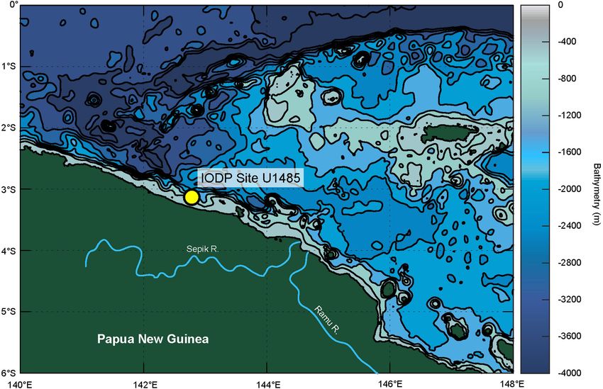
a 60 6 e 60 6
Se
radiative forcing (W m–2)
radiative forcing (W m–2)
radiative forcing (W m–2)
a
Change in mean annual
Change in mean annual
radiative forcing (W m–2)
lati
on ansona us mean
Change in seasonal
Change in seasonal
40 nso
nu l m 4 40 Seasonal minola 4
al i
al in
ins us annual ins tion
on ola m
eas tio ean
20 S n 2 20 Seasona
l insolati 2
in so la ti o n on
n annu a l
Mea Greenhouse gases
0 0 0 0
Greenhouse gases al insolation
Mean annu
–20 –2 –20 –2
b 29.5 32.5 f 32.5
29.5
29.0 32.0 32.0
29.0
Model seasonal SST (°C)
Model seasonal SST (°C)
28.5 31.5 31.5
28.5
28.0 31.0 31.0
SSTSN (°C)
SSTSN (°C)
27.5 30.5 28.0 30.5
27.0 30.0 30.0
27.5
26.5 29.5 29.5
27.0
26.0 IODP site U1485 Mg/Ca SSTSN 29.0 29.0
Accelerated CCSM3 October SST 26.5
25.5 28.5 28.5
c g
1.0 1.0
0.5 0.5
ΔSST (°C)
ΔSST (°C)
0 0
U1485 SSTSN - MASST
–0.5 –0.5
October SST - CCSM3 MASST
d 2.0 h 2.0
1.5 1.5
1 1.0
MASST anomaly (°C)
MASST anomaly (°C)
0.5 0.5
0 0
–0.5 –0.5
–1.0 –1.0
–1.5 –1.5
IODP site U1485 Mg/Ca SAT method MASST
–2.0 CCSM3 October SAT method MASST –2.0
CCSM3 MASST
–2.5 –2.5
–3.0 –3.0
128 126 124 122 120 118 116 12 10 8 6 4 2 0
Age (ka) Age (ka)
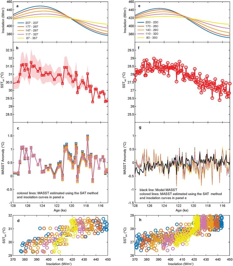
Fig. 1 | Application of SAT method at IODP Site U1485. a, e, Change nearest grid cell from the accelerated CCSM3 simulation (dashed red line).
in seasonal radiative forcing at 3° S (August, Is, left axis, red line; August minus Modern October SSTs (red solid square) and MASSTs (blue solid square) are
mean annual insolation, Is − Is, left axis, pink line) and mean annual radiative shown. c, g, Calculated ΔSST (Methods) for Site U1485 (solid black) and CCSM3
forcing 21,22 , including mean annual insolation ( Is, right axis, blue line) and seasonal output (dashed line). ΔSST is subtracted from SSTSN to convert to
greenhouse gases20 (right axis, grey line). We note that scale differences MASST. d, h, MASST calculated from seasonal SST at Site U1485 (blue solid line
showing the mean annual radiative forcings are an order of magnitude lower with squares) and CCSM3 (dashed lines), plotted with the true model MASST
than the seasonal forcing. b, f, Reconstructed SSTSN at IODP Site U1485 output (cyan). Shaded regions represent the 2 s.e. uncertainty bounds.
(G. ruber ss Mg/Ca, solid red line with squares) and seasonal SSTs from the
between conventionally derived LIG SSTs, hereafter referred to as extent of a proxy record, but rather detects bias toward a particular
seasonally unadjusted SSTs (SSTSN), and insolation averaged over a time of year (Methods). For reconstructions identified as seasonal,
30-day sliding window21,22. Should a record exhibit the strongest cor- we then calculate the linear sensitivity (regression) of LIG SSTSN values
relation with insolation averaged over a 30-day interval (Is) rather than to the seasonal component of the insolation (Is minus Is), where
the mean annual insolation (Is) it is deemed to be seasonally biased. We Is is the identified 30-day insolation curve (Extended Data Fig. 5d, h).
emphasize that the SAT method does not identify the full seasonal This sensitivity (regression coefficient) is then used to transform the
Nature | Vol 589 | 28 January 2021 | 549
Article
a 12 10 8 6 4 2 0 difference between seasonal and mean annual insolation into the
2 difference between SSTSN and MASST values (ΔSST) (Fig. 1c, g). Finally,
we subtract ΔSST from SSTSN to get the MASST values (Fig. 1d, h). We
1 note that this method assumes a linear relationship between SST and
insolation across the year (Methods).
SST anomaly (°C)
0
Western Pacific Mg/Ca SST reconstruction
–1 We demonstrate the utility of this method using a new, centennially
resolved Mg/Ca SSTSN record derived from the planktic foraminifer,
23.5° N–40° N
–2 Globigerinoides ruber (sensu stricto) from IODP Site U1485 (03° 06.16′ S,
142° 47.59′ E, 1,145 m water depth), collected during International
Ocean Discovery Program Expedition 363 and located off the north-
b 2 east coast of Papua New Guinea (Methods, Extended Data Fig. 1). Site
U1485, located in the heart of the Western Pacific Warm Pool (WPWP),
1 is well dated during both the current and previous interglacial peri-
SST anomaly (°C)
ods and glacial terminations (see Methods, Extended Data Figs. 2, 3).
We find a best fit between LIG Mg/Ca SSTSN (Fig. 1b) at Site U1485 with
0
insolation averaged over days-of-year 207 to 237, which roughly corre-
sponds to August, and a SSTSN sensitivity of 0.021 °C/(W m−2) (Extended
–1 Data Table 1). At present, SSTs at Site U1485 lag the insolation forc-
ing by around 1.5 months, suggesting that reconstructed SSTSN at
23.5° S–23.5° N this site is biased towards October SST23. The average uncertainty on
–2
reconstructed Holocene SSTSN and MASST at Site U1485 is ±0.20 °C
and ±0.21 °C (2 standard errors, s.e.), respectively, and LIG SSTSN and
c 2
MASST 2 s.e. uncertainty bounds are each ±0.43 °C.
Like most organisms, planktic foraminifers respond to changes in
1 their environment, such as food availability, light and competition24.
SST anomaly (°C)
Therefore, fluxes of G. ruber ss to the seafloor and thus the record of
0 SSTs preserved in the sediment record may be biased toward certain
times of year. Environmental conditions in the WPWP, however, are
among the most stable in the global ocean25. At present, the average sea-
–1
sonal range of WPWP SST is less than 0.5 °C, suggesting a more limited
impact of seasonality on reconstructed SST23. However, Site U1485, like
40° S–23.5° S
–2 most other marine sites included in global compilations, was recovered
from a margin environment where fast sediment accumulation rates
offer high-resolution, expanded interglacial sections, but seasonality
d 2
in SST and other environmental parameters are intensified relative to
conditions further offshore (Methods).
1 Application of the SAT method to data from Site U1485 demon-
SST anomaly (°C)
strates that Mg/Ca SSTSN values from this location are seasonally biased
0 (Fig. 1b), and that the evolution of MASST during the LIG was one of
warming, rather than cooling, consistent with rising mean annual inso-
lation across this time interval (Fig. 1a–d). Assuming the same seasonal
–1
bias and SSTSN sensitivity to insolation, similar results emerge from
Proxy SSTSN Model SSTSN the Holocene data (Fig. 1e–h). However, seasonality is lower during
–2 40° S–40° N the Holocene owing to the Earth’s low eccentricity state and unlike
Proxy MASST Model MASST
during the LIG, Holocene greenhouse gas forcing is non-negligible and
12 10 8 6 4 2 0
seems to offset cooling driven by the decrease in seasonal insolation in
Age (ka)
the mid- to late Holocene. The combined effects explain the absence
Fig. 2 | Regional seasonal and mean annual temperature reconstructions. of a decrease in SSTSN at Site U1485 and the subdued cooling trends
a, Proxy SST anomaly stacks (n = 11) for the northern mid-latitudes (solid lines with at other sites in the western Pacific Ocean26. Compared with the LIG,
squares) plotted with mean annual and seasonal SST from Trace4, averaged over Holocene MASSTs at Site U1485 show a stronger increasing trend in the
23.5° N to 40° N (thin lines). Trace MASST values are from the full Trace experiment, mid- to late interglacial period, beginning 6.5 ka (Fig. 1d–h), consistent
including orbital, greenhouse gas, ice, and meltwater forcing (Trace-all) and Trace
with the observed rise in Holocene greenhouse gases and mean annual
seasonal SST is from the Trace single-forcing experiment in which only orbital
insolation at this time (Fig. 1e).
forcing varies. SSTSN = August–November. b, Proxy SST stacks for the tropics
(SSTSN: n = 28, MASST: n = 31) (solid lines with squares) plotted with Trace4 seasonal
(Trace-orb) and mean annual (Trace-all) SST averaged over 23.5° S to 23.5° N (thin
Validating the SAT method
lines). SSTSN = August–November. c, Proxy SST stacks for the southern mid-latitudes
(n = 2) (solid lines with squares) plotted with Trace4 seasonal (Trace-orb) and mean To independently test the efficacy of the SAT method, we apply it to
annual (Trace-all) SST averaged over 40° S to 23.5° S (thin lines). SSTSN = November– monthly SST anomaly data from a transient model simulation, where
January. d, Full proxy SST compilations (SSTSN: n = 41, MASST: n = 44) (solid lines with the seasonal and mean annual temperatures are known. As LIG SSTs
squares) plotted with Trace4 seasonal (Trace-orb) and mean annual (Trace-all) SST are a necessity for applying our method, we validated our approach
averaged over 40° S to 40° N (thin lines). SSTSN = August–November, shown in red; using the output from a transient experiment of the past 300 ka in the
MASST is shown in blue. Shaded areas represent the 1 s.e. bounds. Trace data were fully coupled National Center for Atmospheric Research Community
smoothed by taking a 60-yr moving mean.
550 | Nature | Vol 589 | 28 January 2021
Climate System Model, version 3 (NCAR-CCSM3) model under realistic
orbital and greenhouse gas forcings, with an acceleration of 100 times                          1.0
                                                                                                           a
on the forcing7 (Methods) (Fig. 1). We use the SSTs from the nearest grid
cell to site U1485 and follow the same method of converting model                               0.5
October SST anomalies to MASST anomalies that we applied to the

                                                                            SST anomaly (°C)
SSTSN reconstruction from Site U1485. As shown in Fig. 1, the SAT method                         0                  MR13
successfully converts October SSTs to mean annual SSTs within error                                                 Temperature 12k
of the true mean annual model output for both the Holocene and LIG                             –0.5
(Fig. 1b–d, f–h).                                                                                                                                        Pages 2k
                                                                                               –1.0                                                   Instrumental       1.0

Building regional SST stacks                                                                   –1.5                                                                      0.5
Given the success of the SAT method in reproducing simulated MASSTs
                                                                                                           b

                                                                                                                                                                                      SST anomaly (°C)
from seasonal SSTs as well as the consistency of our results from Site                         –2.0                                                                      0
U1485 with mean annual forcings, we apply the method to a suite of
eight additional planktic foraminifer Mg/Ca and eleven alkenone                                                                                                          –0.5
SSTSN records from 40° S to 40° N that have Holocene and LIG sections
(Extended Data Table 1, Extended Data Fig. 6, Methods). To increase                                                 SSTSN (this study)                                   –1.0
data coverage over the Holocene, we transfer the inferred seasonality                                               MASST (this study)
                                                                                                0.5
and SSTSN sensitivities to insolation to 24 additional locations that                                                                                                    –1.5
have Holocene but no LIG reconstructions within the same region.                                                                                      MASST
Datasets with better than 2 kyr resolution across at least two-thirds of                                                            (40° S–40° N, Trace-GHG)             –2.0
the LIG and/or Holocene are included. We exclude records from higher                             0
                                                                                                           c
latitudes owing to the scarcity of LIG records and the proximity of many
                                                                            SST anomaly (°C)

                                                                                                                                                                                                              Change in radiative forcing by greenhouse gases (W m–2)
                                                                                                                                                                                                         3
of the records that do contain reasonably resolved LIG and Holocene                                                                                    MASST
sections to ocean fronts where SST can be strongly affected by ocean                           –0.5                                    (40° S–40° N, Trace-all)
                                                                                                                                                       MASST
dynamics. We find that the vast majority of SSTSN records examined,
                                                                                                                                             (Global, Trace-all)
whether derived by Mg/Ca or alkenone palaeothermometry, track                                                                                                                                            2
boreal summer and autumn insolation (Extended Data Fig. 7, Extended
                                                                                               –1.0
Data Table 1). We therefore argue that reconstructions based on stacked
                                                                                                                      Sea level39              Sea level38               20
Mg/Ca and alkenone SSTSN records are biased toward boreal summer/
autumn temperatures, and do not reflect the annual mean.                                                                                                                 0                               1
                                                                                               –1.5        d
   From these datasets, we built regional composite stacks of SSTSN

                                                                                                                                                                               Sea level (m)
and MASST for both the LIG and Holocene time intervals for three                                                                                                         –20
latitudinal bands: the tropics (23.5° S–23.5° N), Northern Hemisphere
                                                                                                                                                                         –40                             0
mid-latitudes (23.5–40° N), and Southern Hemisphere mid-latitudes
(23.5–40° S) (Fig. 2). To account for uncertainty in age–depth models
                                                                                                                                                                         –60
and the necessity of including low-resolution records (>500 yr reso-                                                     Radiative forcing (CO2 + CH4 +N2O)
lution) to increase data coverage, we binned the data at 1,000-year                                                                                                      –80                             –1
intervals. The resulting regional stacks demonstrate that Holocene                                    12       10         8           6           4          2       0
climate, at least between 40° S and 40° N, has been warming since the                                                               Age (ka)
early Holocene, with no evidence for an early- or mid-Holocene thermal      Fig. 3 | Holocene warming driven by retreating ice sheets and rising
maximum in the annual mean in the tropics or Northern Hemisphere            greenhouse gases. a, Previous global proxy temperature reconstructions for the
stacks. The Southern Hemisphere ‘stack’ does exhibit an early-Holocene      Holocene, Temperature 12k (refs. 1,2) and MR133, and the past 2 kyr (Pages 2k)10,
thermal maximum but is highly uncertain owing to limited (n = 2) record     with 1σ uncertainty shaded. The instrumental record29 since 1850 is shown in
availability and the proximity of one of the two records (MD97-2121)        black. b, Seasonal (n = 41) and mean annual (n = 44) SST reconstructions (this
to oceanographic fronts. Early Holocene (about 10–5 ka) warmth is           study) for 40° S to 40° N and the Pages 2k10 reconstruction, with 1 s.e. and 1σ
identified at all latitudes in the SSTSN stacked records, a result sug-     uncertainties shaded, respectively. The instrumental record29 since 1850 is shown
gesting that the Holocene thermal maximum is a seasonal, rather than        in black. c, Simulated Holocene mean annual global (green) and 40° S to 40° N
                                                                            (dark blue) MASSTs from Trace-all (60-yr moving average)4. Also shown are
mean annual, feature driven by the early Holocene maximum in boreal
                                                                            simulated 40° S–40° N MASSTs for the Trace-GHG single forcing experiment
summer insolation.
                                                                            (light blue; 60-yr moving average). d, Holocene sea level curves38,39, representative
   The large-scale features of our 40° S–40° N stacked record of
                                                                            of changing global ice volume, and the combined evolution of CO2, CH4 and N2O
SSTSN—early interglacial warmth followed by cooling—are broadly             radiative forcing20. All reconstructions are referenced to their respective values
comparable to previous global compilations of Holocene surface tem-         averaged between 0 and 1 ka.
peratures1–3 (Fig. 3a, b). The Holocene global compilations are based
on a variety of temperature-sensitive proxies, including non-marine
archives. The MR13 (https://science.sciencemag.org/highwire/file-           to strong nonlinearities in the response of terrestrial surface air tem-
stream/594506/field_highwire_adjunct_files/1/Marcott.SM.database.           peratures to insolation forcing.
S1.xlsx) compilation3 is largely derived from marine archives (about
80%), of which the majority are Mg/Ca and alkenone. In contrast, just
31% of the records in the Temperature 12k (https://www.ncdc.noaa.           Holocene conundrum revisited
gov/paleo-search/study/27330) compilation1,2 are marine. Therefore,         Confidence in our method and its application to the Mg/Ca and alk-
if our interpretation is correct, it is possible that a substantial swath   enone SSTSN records compiled here is buoyed by the resemblance
of terrestrial proxies may also exhibit seasonal biases similar to those    during the Holocene between our mean annual tropics-only and
explored here. Alternatively, local and/or regional dynamics may lead       40° S–40° N stacked records (Fig. 2b, d) and corresponding MASSTs

                                                                                                                                    Nature | Vol 589 | 28 January 2021 | 551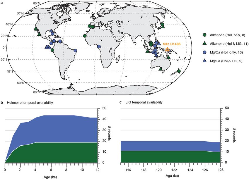
Article
a LIG age (ka) b LIG age (ka)
127 125 123 121 119 117 115 127 125 123 121 119 117 115
2.5
50
Change in seasonal insolation (W m–2)
LIG Holocene
2.0
40
SSTSN anomaly (°C)
1.5
30
1.0
20
0.5 10
0 0
–0.5 –10
–1.0 –20
12 10 8 6 4 2 0 12 10 8 6 4 2 0
c 127 125 123 121 119 117 115 d 127 125 123 121 119 117 115
20
1.5
10
1.0 0
MASST anomaly (°C)
–10
0.5
Sea level (m)
–20
0
–30
–0.5 –40
LIG37
–1.0 –50 Holocene39
–60 Holocene38
–1.5
–70
12 10 8 6 4 2 0 12 10 8 6 4 2 0
Holocene age (ka) Holocene age (ka)
Fig. 4 | Evolution and drivers of Holocene and LIG SST. LIG, triangles; anomalies (LIG n = 13; Holocene n = 31). d, Sea level reconstructions for the
Holocene, squares. a, Tropical SSTSN anomalies (LIG n = 10; Holocene n = 28). LIG (triangles)37 and current interglacial period38,39 (dashed and solid lines).
b, Average tropical June–September insolation21,22. c, Tropical MASST All proxy stacks show 1 s.e. bounds shaded.
in the unaccelerated transient simulation Trace with all climate forc- the Northern Hemisphere monsoon regions and the high north-
ings (Trace-all) (https://www.cgd.ucar.edu/ccr/TraCE/) (Fig. 2a–d, ern latitudes. For example, a wide range of palaeoclimate archives,
Fig. 3c)4. The tropics-only and 40° S–40° N stacked SST reconstruc- including palaeo-lake levels, pollen and geochemical data, document
tions are within error of the simulated evolution of mean tropical and early Holocene increases in North African monsoon precipitation
40° S–40° N SSTs. In the model, annual temperature change averaged and subsequent greening of the Sahara (the Holocene African humid
between 40° S and 40° N is analogous to simulated global SSTs (Fig. 3c). period)30, large swaths of northwest Canada transitioned from tundra
This suggests that the mean trends of both our tropics-only and full to forest31, and glaciers retreated in the Arctic32. These observations
stacked datasets are representative of global mean trends. can be, and in fact have always been, attributed to the early Holocene
Now that the proxy data and model simulations are directly compa- maximum in boreal summer insolation. Summer insolation, not the
rable, we can further isolate the primary forcings responsible for rising annual mean, has long been deemed the ‘pacemaker’ of the ice ages33–35
mean annual temperatures across the Holocene by taking advantage and the monsoons36. Thus, reconstructions and simulations of mean
of single forcing sensitivity experiments that accompany Trace-all, in annual temperatures are important, but are not fully descriptive of
which orbital, greenhouse gases, ice and meltwater forcings are inde- past climates.
pendently changed4 (Fig. 3d). We find that the late Holocene (6.5–0 ka) The lack of a thermal maximum in global mean annual temperatures
rise in global temperatures can be attributed solely to rising atmos- is not limited to the Holocene interglacial period. Like the Holocene
pheric greenhouse gas levels (Fig. 3c), whereas the early Holocene thermal maximum, we show that the LIG thermal maximum8 is a sea-
(12–6.5 ka) increase arises via a combination of mechanisms, including sonal feature (Fig. 4a, b), coinciding with maximum boreal summer
greenhouse gas, ice and orbital forcings, as was suggested previously4. insolation (120–128 ka), and is not observed in the LIG mean annual tem-
Although the source of the rising late Holocene greenhouse gas con- perature stack (Fig. 4c). Owing to the relative lack of LIG records from
centrations is still contentious27,28, whether natural or anthropogenic the mid-latitudes, we focus on the tropics, which are well documented
in origin, we estimate a 0.25 ± 0.21 °C increase in global mean annual with 13 records from the Indo-Pacific warm pool, eastern tropical Pacific
surface temperature between binned data at 6.5 ka and 0.5 ka (Fig. 3b), and tropical Atlantic oceans. We find that maximum boreal summer/
that is, about a quarter of the post-industrial warming29. autumn SSTs were 1.24 ± 0.69 °C warmer during the LIG relative to
maximum Holocene boreal summer/autumn SSTs, consistent with
higher June–September insolation during the LIG (Fig. 4a).
Seasonal origin of interglacial peak warmth Average LIG tropical MASSTs were 0.62 ± 0.60 °C warmer than late
A seasonal origin for the Holocene thermal maximum in global Holocene MASSTs averaged between 0 and 1 ka, but the difference in
reconstructions does not negate the impact of the event on regional mean annual radiative forcing (+1.4 W m−2 for the LIG) is inadequate to
climates. Evidence of its impact is widespread, particularly within explain this offset. We therefore hypothesize that the Holocene was
552 | Nature | Vol 589 | 28 January 2021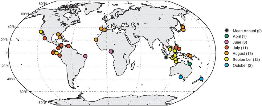
cooler than the LIG largely owing to differences in ice volume, deter-                           10.   PAGES 2k Consortium. Consistent multidecadal variability in global temperature
                                                                                                       reconstructions and simulations over the Common Era. Nat. Geosci. 12, 643–649
mined not by differences in interglacial forcings, but by the dynamics of                              (2019).
their preceding deglaciations. The penultimate deglaciation occurred                             11.   Marsicek, J., Shuman, B. N., Bartlein, P. J., Shafer, S. L. & Brewer, S. Reconciling divergent
more rapidly than the last; ice sheets shrank to near-modern levels by                                 trends and millennial variations in Holocene temperatures. Nature 554, 92–96 (2018).
                                                                                                 12.   Rodriguez, L. G. et al. Mid-Holocene, coral-based sea surface temperatures in the
the onset of the LIG37, whereas only about half their retreat occurred                                 western tropical Atlantic. Paleoceanogr. Paleoclimatol. 34, 1234–1245 (2019).
before the start of the Holocene38,39 (Fig. 4d). Greater ice extent dur-                         13.   Timmermann, A., Sachs, J. & Timm, O. E. Assessing divergent SST behavior during the last
ing the early Holocene would have increased the surface albedo of                                      21 ka derived from alkenones and G. ruber-Mg/Ca in the equatorial Pacific. Paleoceanogr.
                                                                                                       Paleoclimatol. 29, 680–696 (2014).
Earth relative to the LIG and cooled the planet. Holocene temperatures                           14.   Leduc, G., Schneider, R., Kim, J.-H. & Lohmann, G. Holocene and Eemian sea surface
therefore began cooler than during the LIG, a fortuitous advantage for                                 temperature trends as revealed by alkenone and Mg/Ca paleothermometry. Quat. Sci.
our warming world, but increased more rapidly across the interglacial                                  Rev. 29, 989–1004 (2010).
                                                                                                 15.   Liu, Y. et al. A possible role of dust in resolving the Holocene temperature conundrum.
period owing to mid- to late-Holocene increases in atmospheric green-                                  Sci. Rep. 8, 4434 (2018).
house gas concentrations.                                                                        16.   Park, H.-S., Kim, S.-J., Stewart, A. L., Son, S.-W. & Seo, K.-H. Mid-Holocene Northern
   In summary, our new method suggests (1) that the majority of                                        Hemisphere warming driven by Arctic amplification. Sci. Adv. 5, eaax8203 (2019).
                                                                                                 17.   Affolter, S. et al. Central Europe temperature constrained by speleothem fluid inclusion
high-resolution palaeotemperature reconstructions from the marine                                      water isotopes over the past 14,000 years. Sci. Adv. 5, eaav3809 (2019).
realm based on Mg/Ca and alkenone palaeothermometry reflect the                                  18.   Martin, C. et al. Early Holocene Thermal Maximum recorded by branched tetraethers and
evolution of seasonal, rather than mean annual, temperatures and (2)                                   pollen in Western Europe (Massif Central, France). Quat. Sci. Rev. 228, (2020).
                                                                                                 19.   Longo, W. M. et al. Insolation and greenhouse gases drove Holocene winter and spring
that there is no thermal maximum in global mean annual tempera-                                        warming in Arctic Alaska. Quat. Sci. Rev. 242, 106438 (2020).
tures during the first half of the last and current interglacial periods.                        20.   Köhler, P., Nehrbass-Ahles, C., Schmitt, J., Stocker, T. F. & Fischer, H. A. 156 kyr smoothed
It follows, therefore, that the post-industrial increase in global mean                                history of the atmospheric greenhouse gases CO2, CH4, and N2O and their radiative
                                                                                                       forcing. Earth Syst. Sci. Data 9, 363–387 (2017).
annual surface temperatures rose from the warmest background state                               21.   Huybers, P. & Eisenman, I. (eds) NOAA/NCDC Paleoclimatology Program, http://eisenman.
of the Holocene, making current temperatures the warmest observed                                      ucsd.edu/code/daily_insolation.m (IGBP PAGES/World Data Center for Paleoclimatology,
over the past 12,000 years and probably reaching the warmth of the                                     2006).
                                                                                                 22.   Berger, A. Long-term variations of daily insolation and Quaternary climatic changes.
LIG. Given that previous interglacial periods were forced similarly, we                                J. Atmos. Sci. 35, 2362–2367 (1978).
speculate that an early thermal maximum may also be lacking in global                            23.   Freeman, E. et al. ICOADS Release 3.0: a major update to the historical marine climate
                                                                                                       record. Int. J. Climatol. 37, 2211–2232 (2017).
mean annual temperature in all interglacial periods. This suggests
                                                                                                 24.   Be, A. & Hamilton, W. H. Ecology of recent planktonic foraminifera. Micropaleontology 13,
that the maximum mean annual global temperature in each glacial                                        87–106 (1967).
cycle is reached not in the middle of the interglacial period when the                           25.   De Deckker, P. The Indo-Pacific warm pool: critical to world oceanography and world
                                                                                                       climate. Geosci. Lett. 3, 20 (2016).
boreal summer insolation peaks, but instead thousands of years later,
                                                                                                 26.   Moffa-Sanchez, P., Rosenthal, Y., Babila, T. L., Mohtadi, M. & Zhang, X. Temperature
which should be considered when using these periods as analogues of                                    evolution of the Indo-Pacific warm pool over the Holocene and the last deglaciation.
future warming.                                                                                        Paleoceanogr. Paleoclimatol. 34, 1107–1123 (2019).
                                                                                                 27.   Ruddiman, W., He, F., Vavrus, S. & Kutzbach, J. The early anthropogenic hypothesis: a
                                                                                                       review. Quat. Sci. Rev. 240, 106386 (2020).
                                                                                                 28.   Studer, A. S. et al. Increased nutrient supply to the Southern Ocean during the Holocene
Online content                                                                                         and its implications for the pre-industrial atmospheric CO2 rise. Nat. Geosci. 11, 756–760
                                                                                                       (2018).
Any methods, additional references, Nature Research reporting sum-
                                                                                                 29.   Cowtan, K. & Way, R. G. Coverage bias in the HadCRUT4 temperature series and its
maries, source data, extended data, supplementary information,                                         impact on recent temperature trends. Q. J. R. Meteorol. Soc. 140, 1935–1944 (2014).
acknowledgements, peer review information; details of author contri-                             30.   Pausata, F. S. R. et al. The greening of the Sahara: past changes and future implications.
                                                                                                       One Earth 2, 235–250 (2020).
butions and competing interests; and statements of data and code avail-
                                                                                                 31.   Ritchie, J. C., Cwynar, L. C. & Spear, R. W. Evidence from north-west Canada for an early
ability are available at https://doi.org/10.1038/s41586-020-03155-x.                                   Holocene Milankovitch thermal maximum. Nature 305, 126–128 (1983).
                                                                                                 32.   McKay, N. P., Kaufman, D. S., Routson, C. C., Erb, M. P. & Zander, P. D. The onset and rate of
                                                                                                       Holocene neoglacial cooling in the Arctic. Geophys. Res. Lett. 45, 12487–12496 (2018).
1.   Kaufman, D. et al. Holocene global mean surface temperature, a multi-method                 33.   Hays, J. D., Imbrie, J. & Shackleton, N. J. Variations in the Earth’s orbit: pacemaker of the
     reconstruction approach. Sci. Data 7, 201 (2020).                                                 Ice Ages. Science 194, 1121–1132 (1976).
2.   Kaufman, D. et al. A global database of Holocene paleotemperature records. Sci. Data 7,     34.   Milankovitch, M. Kanon Der Erdbestrahlung Und Seine Anwendung Auf Das
     183 (2020).                                                                                       Eiszeitenproblem (Mihaila Ćurčića, 1941).
3.   Marcott, S. A., Shakun, J. D., Clark, P. U. & Mix, A. C. A reconstruction of regional and   35.   Imbrie, J. et al. On the structure and origin of major glaciation cycles. 1. Linear responses
     global temperature for the past 11,300 years. Science 339, 1198–1201 (2013).                      to Milankovitch forcing. Paleoceanogr. Paleoclimatol. 7, 701–738 (1992).
4.   Liu, Z. et al. The Holocene temperature conundrum. Proc. Natl Acad. Sci. USA 111,           36.   Wang, P. X. et al. The global monsoon across time scales: mechanisms and outstanding
     E3501–E3505 (2014).                                                                               issues. Earth Sci. Rev. 174, 84–121 (2017).
5.   Brierley, C. M. et al. Large-scale features and evaluation of the PMIP4-CMIP6               37.   Clark, P. U. et al. Oceanic forcing of penultimate deglacial and last interglacial sea-level
     mid-Holocene simulations. Clim. Past Discuss. 2020, 1–35 (2020).                                  rise. Nature 577, 660–664 (2020).
6.   Varma, V., Prange, M. & Schulz, M. Transient simulations of the present and the last        38.   Lambeck, K., Rouby, H., Purcell, A., Sun, Y. & Sambridge, M. Sea level and global ice
     interglacial climate using the Community Climate System Model version 3: effects of               volumes from the Last Glacial Maximum to the Holocene. Proc. Natl Acad. Sci. USA 111,
     orbital acceleration. Geosci. Model Dev. 9, 3859–3873 (2016).                                     15296–15303 (2014).
7.   Lu, Z., Liu, Z., Chen, G. & Guan, J. Prominent precession band variance in ENSO intensity   39.   Grant, K. M. et al. Rapid coupling between ice volume and polar temperature over the
     over the last 300,000 years. Geophys. Res. Lett. 46, 9786–9795 (2019).                            past 150,000 years. Nature 491, 744–747 (2012).
8.   Hoffman, J. S., Clark, P. U., Parnell, A. C. & He, F. Regional and global sea-surface
     temperatures during the last interglaciation. Science 355, 276–279 (2017).                  Publisher’s note Springer Nature remains neutral with regard to jurisdictional claims in
9.   Mann, M. E. et al. Proxy-based reconstructions of hemispheric and global surface            published maps and institutional affiliations.
     temperature variations over the past two millennia. Proc. Natl Acad. Sci. USA 105,
     13252–13257 (2008).                                                                         © The Author(s), under exclusive licence to Springer Nature Limited 2021

                                                                                                                                         Nature | Vol 589 | 28 January 2021 | 553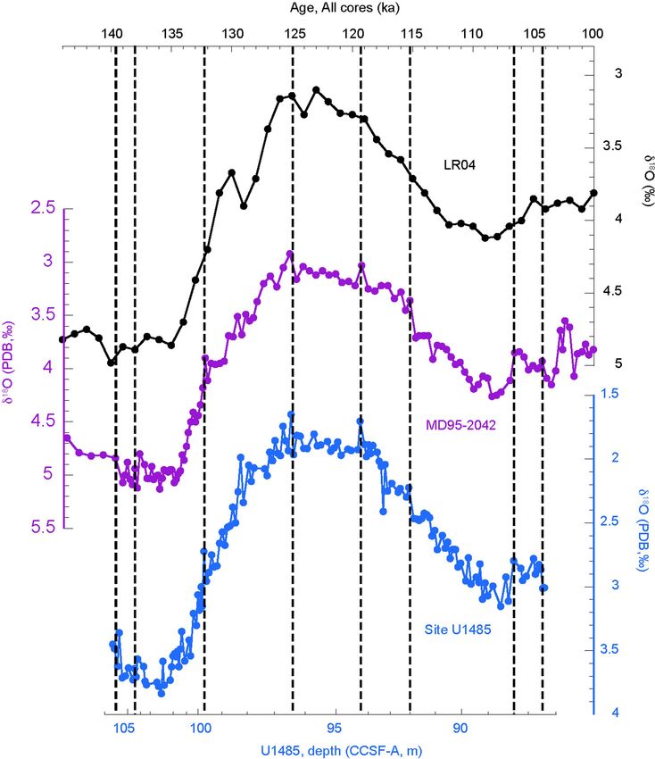
Article
Methods
Foraminifer preservation. Foraminifer preservation at IODP Site U1485
Site U1485 is excellent and glassy, with no evidence of dissolution, recrystalliza-
Age–depth model. We measured 20 accelerator mass spectrome- tion or cementation48.
try radiocarbon dates on G. ruber (>150 μm) and converted them to
calendar ages using the IntCal13 calibration curve40. Corrections for The SAT method
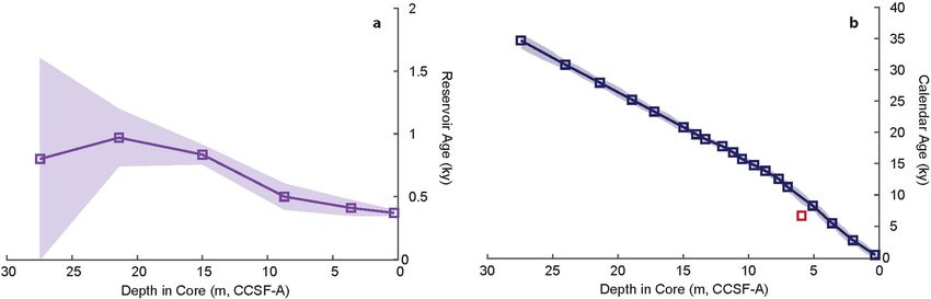
the reservoir age (the radiocarbon age difference between the at- Identifying seasonal bias. The method presented here for identifying
mosphere and ocean) were determined by measuring 18 accelerator seasonal bias in temperature-sensitive proxy records relies on the avail-
mass spectrometry radiocarbon measurements on wood fragments, ability of records that span the LIG. The LIG between 127 ka and 115 ka is
containing atmospheric radiocarbon, picked out of the >63 μm sam- a uniquely useful interval because (1) the high eccentricity state leads
ple coarse fractions. Twelve of the wood 14C dates were removed from to strong seasonality, which makes proxy seasonal biases, if present,
reservoir age calculations following two criteria: the wood 14C age easier to diagnose and (2) greenhouse gas concentrations and sea level37
was older than the coexisting planktonic foraminifera 14C age41 and were stable across this time interval, which means that SST change can
wood 14C dates that suggest lower than present surface reservoir ages be attributed solely to variations in solar insolation. We thus explicitly
(
study/6355?siteId=56411, https://doi.org/10.1594/PANGAEA.882099,                               uncertainty of the individual records, including calibration error and
www.ncdc.noaa.gov/paleo-search/study/6247?siteId=30616, http://                                regression error for the transformed MASST estimates, the number of
ncdc.noaa.gov/pub/data/paleo/contributions_by_author/lea2000/                                  records, and the variability among records within each stack. For each
readme_lea2000.txt, https://doi.org/10.1594/PANGAEA.819829, http://                            record, we estimate a calibration error ec derived as the standard error
ncdc.noaa.gov/pub/data/paleo/paleocean/sediment_files/complete/                                of the SSTSN anomalies calculated using two calibrations (Mg/Ca from
odp1012-tab.txt and http://ncdc.noaa.gov/pub/data/paleo/contribu-                              Anand et al.91 and BAYMAG92; alkenone from Prahl et al.94 & BAY-
tions_by_author/yamamoto2007/yamamoto2007.txt).                                                SPLINE95). For MASST estimates, we assess the error on the regression
                                                                                               coefficient er between the seasonal component of the insolation of best
Selection criteria. The purpose of the temperature reconstructions                             fit (Is − Is) and SSTSN. er is determined via a jackknife cross-validation
presented in this paper is to evaluate multi-millennial temperature                            procedure that estimates variability in MASST derived by fitting insola-
change over the Holocene and the LIG. We therefore include records                             tion to n − 1 proxy data points. For each regional stack, we add an addi-
that extend over at least two-thirds of the LIG and/or Holocene inter-                         tional error term that quantifies the variability among the available re-
vals, with at least 2 kyr resolution. Most records, however, are better                        cords, calculated as the standard error of the mean SST (that is, the
resolved, with an average resolution for Holocene records of 330 yr and                        standard deviation of the SST records at each binned data point divided
LIG records of 850 yr. We use the new age–depth models generated for                           by the square root of the number of records in each stack). The uncer-
the Holocene records included in the Temperature 12k database2 and                             tainty on the final stack is calculated as the square root of the sum of the
the original age–depth models for sites that were not included in this                         errors on each regional stack squared. All SST stacks (regional and the
database and all LIG sections.                                                                 full 40° S–40° N stack) are plotted in figures with the 1 s.e. bound shaded.

Proxy temperature calibrations. We apply the traditional multi-species                         Transient model simulations
calibration from Anand et al.91 that assumes that foraminiferal Mg/Ca                          Our model is the National Center for Atmospheric Research Community
is dominantly controlled by temperature (Mg/Ca = 0.38e0.09SST) as well                         Climate System Model, version 3 (NCAR-CCSM3)97. The atmospheric
as a recent, multivariate calibration (BAYMAG) that also considers the                         model has a ~3.75° latitude/longitude resolution (T31) and the ocean
impacts of salinity, pH, dissolution, and cleaning methods on planktic                         model has a ~3.6° longitudinal resolution, a variable latitudinal resolu-
foraminifer Mg/Ca (ref. 92) (Extended Data Fig. 4; Methods). When ex-                          tion (~0.9° near the Equator, gx3v5). A 3000-year-long transient simula-
pressed as temperature anomalies, the SSTSN estimates for the LIG and                          tion (ORB, ORB+GHG) was performed in which the orbital forcing and
Holocene time intervals are largely consistent between the calibrations                        greenhouse gases concentration were prescribed as in the past 300,000
(Extended Data Fig. 4; Methods). Final SSTSN anomalies represent the                           years (300 ka to the present day), but with an acceleration factor of 100
average value from the two calibrations.                                                       (ref. 7). The tropical–subtropical climate and surface ocean are expected
   At IODP Site U1485 we tested a third calibration93 (GE2019, Mg/                             to reach quasi-equilibrium with this acceleration and therefore their
Ca = e[0.036(S − 35) + 0.064SST − 0.87(pH = −8) − 0.03], where S is salinity) (Extended Data   evolution is affected little by the acceleration7,98. Indeed, the Holocene
Fig. 4). SSTSN anomalies calculated via this method are also consistent                        part of the simulation compares well with the transient simulation in
with results from the Anand et al.91 and BAYMAG92 calibrations.                                the same model without acceleration4.
                                                            k′
   The alkenone unsaturation index (U37                        ) is converted to SSTSN using
                       94
the Prahl et al. palaeotemperature equation and the BAYSPLINE                                  Geographic variability in proxy seasonal bias
calibration programme95. Anomalies resulting from each calibration                             High-resolution marine sediment records. The average annual range
are averaged.                                                                                  in sea surface temperature in the WPWP (
Article
rates offer high-resolution, expanded sections, come with the cost 44. Lisiecki, L. E. & Raymo, M. E. A Pliocene-Pleistocene stack of 57 globally distributed benthic
δ18O records. Paleoceanogr. Paleoclimatol. 20, https://doi.org/10.1029/2004PA001071
of increased likelihood of seasonal bias in palaeo-reconstructions. (2005).
Recovery of LIG sections in these locations is therefore essential to 45. Shackleton, N. J., Hall, M. A. & Vincent, E. Phase relationships between millennial‐scale
leverage high-fidelity reconstructions of mean annual conditions. events 64,000–24,000 years ago. Paleoceanogr. Paleoclimatol. 15, 565–569 (2000).
46. Rosenthal, Y., Boyle, E. A. & Slowey, N. Temperature control on the incorporation of
Recovery of complementary, lower-resolution, offshore sites would magnesium, strontium, fluorine, and cadmium into benthic foraminiferal shells from
also be advisable. Little Bahama Bank: prospects for thermocline paleoceanography. Geochim.
Cosmochim. Acta 61, (1997).
47. Rosenthal, Y., Field, M. P. & Sherrell, R. M. Precise determination of element/calcium ratios
The Southern Hemisphere temperature conundrum. The lack of a in calcareous samples using sector field inductively coupled plasma mass spectrometry.
long-term warming trend in Holocene SSTSN records from the Southern Anal. Chem. 71, 3248–3253 (1999).
Hemisphere is often used to support a lack of summer/autumn biases 48. Rosenthal, Y., Holbourn, A. E., Kulhanek, D. K. & Expedition 363 Scientists. Western Pacific
Warm Pool. In Proc. IODP Vol. 363, https://doi.org/10.14379/iodp.proc.363.2018
on global proxy temperature reconstructions1. The argument goes that (International Ocean Discovery Program, 2018).
if proxies are summer/autumn-biased in the Northern Hemisphere, 49. Minoshima, K., Kawahata, H. & Ikehara, K. Changes in biological production in the mixed
one would expect them to exhibit a similar bias in the Southern Hemi- water region (MWR) of the northwestern North Pacific during the last 27 kyr. Palaeogeogr.
Palaeoclimatol. Palaeoecol. 254, 430–447 (2007).
sphere, and therefore Southern Hemisphere SSTSN records should track 50. Bard, E. et al. Retreat velocity of the North Atlantic polar front during the last deglaciation
rising austral summer/autumn insolation across the Holocene and LIG. determined by 14C accelerator mass spectrometry. Nature 328, 791–794 (1987).
However, when we apply our method to the alkenone SST record from 51. Bard, E., Rostek, F., Turon, J.-L. & Gendreau, S. Hydrological impact of Heinrich events in
the subtropical northeast Atlantic. Science 289, 1321–1324 (2000).
site MD03-2607 recovered from the Great Australian Bight in the South- 52. Martrat, B. et al. Four climate cycles of recurring deep and surface water destabilizations
ern Hemisphere mid-latitudes, we detect bias towards austral spring on the Iberian margin. Science 317, 502–507 (2007).
(boreal autumn). If correct, alkenone producers in this region appar- 53. Rodrigo-Gámiz, M., Martínez-Ruiz, F., Rampen, S. W., Schouten, S. & Sinninghe Damsté,
J. S. Sea surface temperature variations in the western Mediterranean Sea over the last
ently have a different relationship to the seasonal cycle than they do 20 kyr: a dual-organic proxy (UK′37 and LDI) approach. Paleoceanogr. Paleoclimatol. 29,
in the Northern Hemisphere—an interesting, but somewhat puzzling 87–98 (2014).
result. 54. Cacho, I. et al. Dansgaard-Oeschger and Heinrich event imprints in Alboran Sea
paleotemperatures. Paleoceanogr. Paleoclimatol. 14, 698–705 (1999).
The observed SSTSN bias towards austral spring could be an artefact. 55. Isono, D. et al. The 1500-year climate oscillation in the midlatitude North Pacific during
Southern Hemisphere (23.5° S–40° S) Mg/Ca and alkenone datasets the Holocene. Geology 37, 591–594 (2009).
56. Yamamoto, M., Yamamuro, M. & Tanaka, Y. The California current system during the last
from the LIG that pass our inclusion criteria are sparse (n = 1), which
136,000 years: response of the North Pacific High to precessional forcing. Quat. Sci. Rev.
limits our ability to determine whether the identified seasonal bias is 26, 405–414 (2007).
a local phenomenon or spatially widespread. However, sediment trap 57. Herbert, T. D. et al. Collapse of the California Current during glacial maxima linked to
climate change on land. Science 293, 71–76 (2001).
datasets from multiple Southern Hemisphere locations, including
58. Ziegler, M., Nürnberg, D., Karas, C., Tiedemann, R. & Lourens, L. J. Persistent summer
the Chatham Rise (offshore New Zealand)101,102 and along the polar expansion of the Atlantic Warm Pool during glacial abrupt cold events. Nat. Geosci. 1,
front in the south Atlantic Ocean102,103 do show maximum fluxes of 601–605 (2008).
59. Schmidt, M. W., Weinlein, W. A., Marcantonio, F. & Lynch-Stieglitz, J. Solar forcing of
both alkenones and foraminifera to the seafloor during austral spring
Florida Straits surface salinity during the early Holocene. Paleoceanogr. Paleoclimatol.
into early summer (approximately September–December). Although 27, https://doi.org/10.1029/2012PA002284 (2012).
Southern Hemisphere sediment trap datasets are also sparse, the gen- 60. Zhao, M., Beveridge, N. A. S., Shackleton, N. J., Sarnthein, M. & Eglinton, G. Molecular
stratigraphy of cores off northwest Africa: sea surface temperature history over the last
eral agreement between observed modern fluxes of proxy recorders to
80 Ka. Paleoceanogr. Paleoclimatol. 10, 661–675 (1995).
the seafloor and the identified seasonal bias in Southern Hemisphere 61. Schmidt, M. W., Spero, H. J. & Lea, D. W. Links between salinity variation in the Caribbean
LIG SSTSN records lends support to our interpretations. Nevertheless, and North Atlantic thermohaline circulation. Nature 428, 160–163 (2004).
62. Schmidt, M. W. et al. Impact of abrupt deglacial climate change on tropical Atlantic
more data are needed to address these issues fully. We contend that the
subsurface temperatures. Proc. Natl Acad. Sci. USA 109, 14348–14352 (2012).
acquisition of LIG SST records from a variety of Southern Hemisphere 63. Lea, D. W., Pak, D. K., Peterson, L. C. & Hughen, K. A. Synchroneity of tropical and
locations should be a high-priority target for the palaeoclimate com- high-latitude Atlantic tmperatures over the Last Glacial Termination. Science 301,
1361–1364 (2003).
munity in the future. 64. de Garidel-Thoron, T., Beaufort, L., Linsley, B. K. & Dannenmann, S. Millennial-scale
dynamics of the east Asian winter monsoon during the last 200,000 years. Paleoceanogr.
Paleoclimatol. 16, 491–502 (2001).
Data availability 65. Rosenthal, Y., Oppo, D. W. & Linsley, B. K. The amplitude and phasing of climate change
during the last deglaciation in the Sulu Sea, western equatorial Pacific. Geophys. Res.
The datasets generated and compiled for this study are available in Lett. 30, https://doi.org/10.1029/2002GL016612 (2003).
the NOAA Database, World Data Service for Paleoclimatology at https:// 66. Zhao, M., Huang, C.-Y., Wang, C.-C. & Wei, G. A millennial-scale U37K′ sea-surface
temperature record from the South China Sea (8°N) over the last 150 kyr: monsoon and
www.ncdc.noaa.gov/paleo/study/31752. International Comprehen- sea-level influence. Palaeogeogr. Palaeoclimatol. Palaeoecol. 236, 39–55 (2006).
sive Ocean-Atmosphere Data Set data were provided by the National 67. Pelejero, C., Grimalt, J. O., Heilig, S., Kienast, M. & Wang, L. High-resolution UK37
Oceanic and Atmospheric Administration/Oceanic and Atmospheric temperature reconstructions in the South China Sea over the past 220 kyr. Paleoceanogr.
Paleoclimatol. 14, 224–231 (1999).
Research/Earth System Research Laboratories Physical Sciences 68. Benway, H. M., Mix, A. C., Haley, B. A. & Klinkhammer, G. P. Eastern Pacific Warm Pool
Laboratory at https://psl.noaa.gov/. Source data are provided with paleosalinity and climate variability: 0–30 kyr. Paleoceanogr. Paleoclimatol. 21,
this paper. https://doi.org/10.1029/2005PA001208 (2006).
69. Dubois, N., Kienast, M., Normandeau, C. & Herbert, T. D. Eastern equatorial Pacific cold
tongue during the Last Glacial Maximum as seen from alkenone paleothermometry.
Paleoceanogr. Paleoclimatol. 24, https://doi.org/10.1029/2009PA001781 (2009).
Code availability 70. Bolliet, T. et al. Mindanao Dome variability over the last 160 kyr: episodic glacial cooling
of the West Pacific Warm Pool. Paleoceanogr. Paleoclimatol. 26, https://doi.org/10.1029/
A MATLAB code that implements the SAT method is available on GitHub 2010PA001966 (2011).
(https://github.com/sambova/SAT). 71. Kienast, M., Steinke, S., Stattegger, K. & Calvert, S. E. Synchronous tropical South China
Sea SST change and Greenland warming during deglaciation. Science 291, 2132–2134
(2001).
40. Reimer, P. J. et al. Intcal13 and Marine13 radiocarbon age calibration curves 0-50,000 72. Fan, W. et al. Variability of the Indonesian throughflow in the Makassar Strait over the last
years cal BP. Radiocarbon 55, 1869–1887 (2013). 30 ka. Sci. Rep. 8, 5678 (2018).
41. Rafter, P. A., Herguera, J.-C. & Southon, J. R. Extreme lowering of deglacial seawater 73. Weldeab, S., Lea, D. W., Schneider, R. R. & Andersen, N. 155,000 years of west African
radiocarbon recorded by both epifaunal and infaunal benthic foraminifera in a monsoon and ocean thermal evolution. Science 316, 1303–1307 (2007).
wood-dated sediment core. Clim. Past 14, 1977–1989 (2018). 74. Weldeab, S., Schneider, R. R., Kölling, M. & Wefer, G. Holocene African droughts relate to
42. Galbraith, E. D., Kwon, E. Y., Bianchi, D., Hain, M. P. & Sarmiento, J. L. The impact of eastern equatorial Atlantic cooling. Geology 33, 981–984 (2005).
atmospheric pCO2 on carbon isotope ratios of the atmosphere and ocean. Glob. 75. Lea, D. W., Pak, D. K. & Spero, H. J. Climate impact of Late Quaternary equatorial Pacific
Biogeochem. Cycles 29, 307–324 (2015). sea surface temperature variations. Science 289, 1719–1724 (2000).
43. Haslett, J. & Parnell, A. A simple monotone process with application to radiocarbon-dated 76. Lea, D. W. et al. Paleoclimate history of Galápagos surface waters over the last 135,000yr.
depth chronologies. J. R. Stat. Soc. C 57, 399–418 (2008). Quat. Sci. Rev. 25, 1152–1167 (2006).77. Pena, L. D., Cacho, I., Ferretti, P. & Hall, M. A. El Niño–Southern Oscillation–like variability 96. Schneider, T. Analysis of incomplete climate data: estimation of mean values and
during glacial terminations and interlatitudinal teleconnections. Paleoceanogr. covariance matrices and imputation of missing values. J. Clim. 14, 853–871 (2001).
Paleoclimatol. 23, https://doi.org/10.1029/2008PA001620 (2008). 97. Yeager, S. G., Shields, C. A., Large, W. G. & Hack, J. J. The low-resolution CCSM3. J. Clim.
78. Schröder, J. F., Holbourn, A., Kuhnt, W. & Küssner, K. Variations in sea surface hydrology in 19, 2545–2566 (2006).
the southern Makassar Strait over the past 26 kyr. Quat. Sci. Rev. 154, 143–156 (2016). 98. Timmermann, A., Lorenz, S. J., An, S.-I., Clement, A. & Xie, S.-P. The effect of orbital forcing
79. Linsley, B. K., Rosenthal, Y. & Oppo, D. W. Holocene evolution of the Indonesian on the mean climate and variability of the tropical Pacific. J. Clim. 20, 4147–4159 (2007).
throughflow and the western Pacific Warm Pool. Nat. Geosci. 3, 578–583 (2010). 99. Delcroix, T. et al. Sea surface temperature and salinity seasonal changes in the western
80. Bova, S. C. et al. Links between eastern equatorial Pacific stratification and Solomon and Bismarck seas. J. Geophys. Res. Oceans 119, 2642–2657 (2014).
atmospheric CO2 rise during the last deglaciation. Paleoceanogr. Paleoclimatol. 30, 100. Palmer, M. R. & Pearson, P. N. A. 23,000-year record of surface water pH and pCO2 in the
1407–1424 (2015). western equatorial Pacific Ocean. Science 300, 480–482 (2003).
81. Arz, H. W., Pätzold, J. & Wefer, G. Correlated millennial-scale changes in surface 101. Sikes, E. L., O’Leary, T., Nodder, S. D. & Volkman, J. K. Alkenone temperature records and
hydrography and terrigenous sediment yield inferred from last-glacial marine deposits biomarker flux at the subtropical front on the Chatham Rise, SW Pacific Ocean. Deep Sea
off northeastern Brazil. Quat. Res. 50, 157–166 (1998). Res. Part I 52, 721–748 (2005).
82. Weldeab, S., Schneider, R. R. & Kölling, M. Deglacial sea surface temperature and salinity 102. King, A. L. & Howard, W. Planktonic foraminiferal δ13C records from Southern Ocean
increase in the western tropical Atlantic in synchrony with high latitude climate sediment traps: new estimates of the oceanic Suess Effect. Glob. Biogeochem. Cycles 18,
instabilities. Earth Planet. Sci. Lett. 241, 699–706 (2006). GB2007 (2004).
83. Visser, K., Thunell, R. & Stott, L. Magnitude and timing of temperature change in the 103. Park, E. M. Variations In GDGT Flux And TEX Thermometry In Three Distinct Oceanic
Indo-Pacific warm pool during deglaciation. Nature 421, 152–155 (2003). Regimes Of The Atlantic Ocean: A Sediment Trap Study. https://epic.awi.de/id/
84. Lückge, A. et al. Monsoon versus ocean circulation controls on paleoenvironmental eprint/51148/1/EPark_PhDThesis_2019.pdf PhD thesis, University of Bremen (2019).
conditions off southern Sumatra during the past 300,000 years. Paleoceanogr. 104. Amante, C. & Eakins, B. W. ETOPO1 Global Relief Model Converted To PanMap Layer
Paleoclimatol. 24, https://doi.org/10.1029/2008PA001627 (2009). Format. https://doi.org/10.1594/PANGAEA.769615 (NOAA-National Geophysical Data
85. Gibbons, F. T. et al. Deglacial δ18O and hydrologic variability in the tropical Pacific and Center, PANGAEA, 2009).
Indian oceans. Earth Planet. Sci. Lett. 387, 240–251 (2014). 105. Emile-Geay, J., McKay, N. P., Wang, J. & Anchukaitis, K. J. CommonClimate/PAGES2k_
86. Xu, J., Holbourn, A., Kuhnt, W., Jian, Z. & Kawamura, H. Changes in the thermocline phase2 code: first public release https://doi.org/10.5281/zenodo.545815 (2017).
structure of the Indonesian outflow during Terminations I and II. Earth Planet. Sci. Lett.
273, 152–162 (2008).
87. Lawrence, K. T. & Herbert, T. D. Late Quaternary sea-surface temperatures in the western Acknowledgements This research used samples and data provided by the International
Coral Sea: implications for the growth of the Australian Great Barrier Reef. Geology 33, Ocean Discovery Program (IODP). We thank the science party, technical staff and crew of IODP
677–680 (2005). Expedition 363, who together ensured the successful recovery of IODP Site U1485. Funding for
88. Lopes dos Santos, R. A. et al. Abrupt vegetation change after the Late Quaternary this research was provided by NSF grants OCE-1834208 and OCE-1810681, the NSF-sponsored
megafaunal extinction in southeastern Australia. Nat. Geosci. 6, 627–631 (2013). US Science Support Program for IODP, the Institute of Earth, Ocean, and Atmospheric
89. Lopes dos Santos, R. A. et al. Comparison of organic (UK´37, TEXH86, LDI) and faunal Sciences at Rutgers University, the Chinese NSF (grant NSFC41630527), Chinese MOST
proxies (foraminiferal assemblages) for reconstruction of late Quaternary sea surface (grant 2017YFA0603801), the School of Geography, Nanjing Normal University and the
temperature variability from offshore southeastern Australia. Paleoceanogr. USIEF-Fulbright Program.
Paleoclimatol. 28, 377–387 (2013).
90. Pahnke, K. & Sachs, J. P. Sea surface temperatures of southern midlatitudes 0–160 kyr B.P. Author contributions S.B. and Y.R. derived the empirical form of the SAT method. S.B.
Paleoceanogr. Paleoclimatol. 21, https://doi.org/10.1029/2005PA001191 (2006). compiled and analysed the proxy datasets and wrote the first manuscript draft. S.B. and S.P.G.
91. Anand, P., Elderfield, H. & Conte, M. H. Calibration of Mg/Ca thermometry in planktonic collected the geochemical data from Site U1485 under the supervision of Y.R. Z.L. and M.Y.
foraminifera from a sediment trap time series. Paleoceanogr. Paleoclimatol. 18, provided access to and interpretation of model results, and the theory explaining the SAT
https://doi.org/10.1029/2002PA000846 (2003). method. All authors provided review and editing.
92. Tierney, J. E., Malevich, S. B., Gray, W., Vetter, L. & Thirumalai, K. Bayesian calibration of
the Mg/Ca paleothermometer in planktic foraminifera. Paleoceanogr. Paleoclimatol. 34, Competing interests The authors declare no competing interests.
2005–2030 (2019).
93. Gray, W. R. & Evans, D. Nonthermal influences on Mg/Ca in planktonic foraminifera: a Additional information
review of culture studies and application to the Last Glacial Maximum. Paleoceanogr. Supplementary information The online version contains supplementary material available at
Paleoclimatol. 34, 306–315 (2019). https://doi.org/10.1038/s41586-020-03155-x.
94. Prahl, F. G., Muehlhausen, L. A. & Zahnle, D. L. Further evaluation of long-chain alkenones Correspondence and requests for materials should be addressed to S.B.
as indicators of paleoceanographic conditions. Geochim. Cosmochim. Acta 52, Peer review information Nature thanks Jeroen Groeneveld, Jennifer Hertzberg, Feng Zhu, and
2303–2310 (1988). the other, anonymous, reviewer(s) for their contribution to the peer review of this work. Peer
95. Tierney, J. E. & Tingley, M. P. BAYSPLINE: a new calibration for the alkenone reviewer reports are available.
paleothermometer. Paleoceanogr. Paleoclimatol. 33, 281–301 (2018). Reprints and permissions information is available at http://www.nature.com/reprints.You can also read