JOINT ESTIMATION OF ROAD ROUGHNESS FROM CROWD-SOURCED BICYCLE ACCELERATION MEASUREMENTS
←
→
Page content transcription
If your browser does not render page correctly, please read the page content below
ISPRS Annals of the Photogrammetry, Remote Sensing and Spatial Information Sciences, Volume V-4-2021
                                                XXIV ISPRS Congress (2021 edition)

     JOINT ESTIMATION OF ROAD ROUGHNESS FROM CROWD-SOURCED BICYCLE
                       ACCELERATION MEASUREMENTS

                                                           O. Wage1 ∗, M. Sester1
       1
           Institute of Cartography and Geoinformatics, Leibniz University Hannover, Appelstraße 9a, 30167 Hannover, Germany
                                                 - {wage, sester}@ikg.uni-hannover.de

                                                        Commission IV, WG IV/4

KEY WORDS: floating bike data, volunteered geographic information, data integration, cycling comfort

ABSTRACT:

In contrast to cars, route choices for cycling are barely influenced by the respective traffic situation, but to a large extent by the
routes’ comfort. Especially in urban settings with several alternatives, segments with many or long stops at traffic lights and badly
maintained roads are avoided due to a low comfort and cyclists vary from the shortest route. This fact is only indirectly considered
in common navigation applications.
This work aims to integrate surface roughness measurements collected from diverse bicycles to a joint scale via a least-squares
adjustment. Data was collected using smartphones, which were mounted to bike hand bars and measured positions and vertical
accelerations on user’s trips. As this way sensed roughness also depends on the bike setting and type, the resulting values would be
different for different users. Thus, this paper presents a novel approach to harmonize observations from differing sensitive setups.
The basic concept idea of bundle block adjustment is adapted to calibrate a basic scale model and in parallel adjust the observations
of surface roughness to a common scale.
This way a crowd-sourced roughness map can be generated. Such a map can be used to enrich bike focused routing services and
thus encourage cycling in daily live. In addition, it can also be used to derive hints for infrastructure servicing.

       1. INTRODUCTION AND RELATED WORK                                  ies on cycling route choice behavior also taking surface quality
                                                                         into account. In recent years authors like (Broach et al., 2012)
Due to the wide availability on smartphones, navigation applic-          analyze the influence of attributes derived from sensor measure-
ations are no longer used only for driving in unknown surround-          ments on cyclist route choice behavior. They are mostly based
ings, but also for everyday rides by bicycle. In contrast to the         on GPS data and do not specifically take the comfort or sur-
car where route choice is mainly influenced by estimated travel          face quality into account. In the thesis by (van Overdijk, R.P.J.,
time, cyclists rather look also for comfortable routes. Espe-            2016) is claimed that good quality paths and low slopes can be
cially to avoid situations with low comfort like gradients, many         worth more than 4 minutes of travel time reduction, and sur-
or long stops at traffic lights and badly maintained roads, cyc-         face quality is placed in the group of most relevant factors for
lists vary from the shortest route ((McCarthy et al., 2016), (van        comfortable routes. In line with this, (McCarthy et al., 2016)
Overdijk, R.P.J., 2016)). This fact is only indirectly considered        also state that cyclists are quite sensitive to comfort and safety
in common navigation applications.                                       aspects and thus are not only interested in the most direct or
                                                                         fast route. In the stated preference survey of (Stinson, Bhat,
In addition to the ongoing revival and increasing popularity of          2003), after travel time and distance to motorized traffic, also
the bicycle for everyday travel and leisure, this development is         the surface type is of highest interest for cyclists. Further, sur-
also interesting from a public policy perspective, as it can be          face quality seems to be the most important aspect compared to
seen as a way to address widespread urban traffic and related            other comfort measures like hilliness, continuity or delays from
environmental problems. In parallel, new bicycle related busi-           stops. This supports the relevance of smooth surface conditions
nesses arise, such as sharing services for bikes and scooters,           for comfortable bicycle routes.
but also a significant spread of parcel and food deliveries by bi-
cycle. In many regions, this development is intended to be fur-          In order to incorporate these factors into a routing service, it
ther promoted by expanding the corresponding infrastructure,             is necessary to have a preferably complete and up-to-date data-
which requires extensive planning and, in some areas, prioritiz-         base. Information on some of the comfort-relevant aspects can
ation. Options for optimizing the above mentioned services on            be obtained from public or free sources. Gradients, for ex-
the existing infrastructure also depend to a large extent on the         ample, can be derived from globally available surface models,
available data. Detailed mapping and monitoring of the state of          and intersections and traffic signals can now usually be found
infrastructure is therefore crucial for informed decision making         in OpenStreetMap (OpenStreetMap contributors, 2020) (OSM).
in a wide range of mobility domains.                                     However, the surface condition of paths is only partially in-
                                                                         cluded in the latter. There is already a routing service, Komoot
In (Dane et al., 2019) a literature overview is given for different      (komoot GmbH, 2021), based on OSM surface tags, but this
factors influencing cyclists’ route choice in general, although          requires a prior manual labeling of the paths by volunteers.
the focus of the paper is on E-bikes. Although based only on hy-
pothetical routes, (Bovy, Bradley, 1985) is one of the first stud-       Automating the acquisition of surface type and roughness by
∗   Corresponding author                                                 means of the smartphones of volunteer cyclists would therefore

             This contribution has been peer-reviewed. The double-blind peer-review was conducted on the basis of the full paper.
                         https://doi.org/10.5194/isprs-annals-V-4-2021-89-2021 | © Author(s) 2021. CC BY 4.0 License.                    89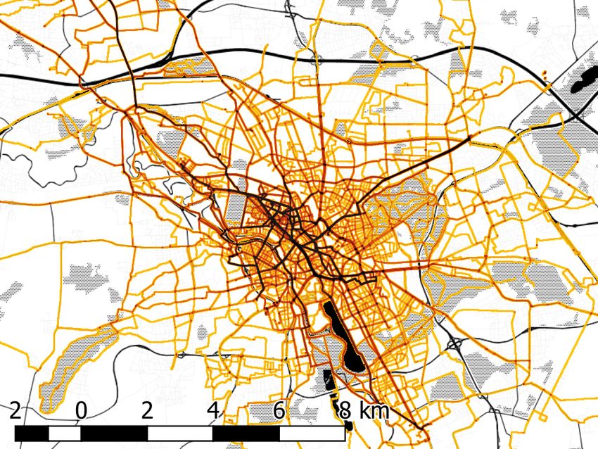
ISPRS Annals of the Photogrammetry, Remote Sensing and Spatial Information Sciences, Volume V-4-2021
                                             XXIV ISPRS Congress (2021 edition)

be desirable, in the sense of crowd-sourcing and volunteered
geographic information. Recently (Brauer et al., 2021) presen-
ted a processing pipeline for bicycle movement data to determ-
ine the flow of different routes, based on the riders speed. In
recent years, applications with different approaches have been
developed in this direction. For example, (Bike Citizens Mobile
Solutions GmbH, 2021) from Austria offers a navigation app
for cyclists similar to Komoot, but also promotes the record-
ing and uploading of the trajectory traveled during use. This
is then analyzed in comparison to the shortest routes to adapt
future recommendations. In this way it can be inferred, at least
implicitly, that short but bypassed route segments are not com-
fortable. The SimRa and RideVibrations projects go one step
further, taking into account other sensors such as acceleration
sensors in addition to the smartphone positioning service. In
SimRa by (Karakaya et al., 2020) from Berlin, data is collected
with the objective of detecting sudden maneuvers due to (near-)
accidents. The aim is to identify dangerous spots. The app and
first collected data are open-source. In (Wage et al., 2020) po-
sition and acceleration data is collected in a very similar way
while riding. However, the focus of the development, data re-
cording and analysis was placed on capturing the way surface
conditions.
Published works such as (Bı́l et al., 2015), (Dawkins et al.,
2011) and (Wage et al., 2020) have shown that vertical accel-
eration measurements on bicycles (but also other vehicles) can
provide information about the roughness (or smoothness) of the
ground. However, scores of roughness were calculated from the
measurements of single, particularly known bicycles. The wide
availability and convenience of smartphones offers much more
possibilities, if used in a crowd-source manner, to achieve much
better coverage and actuality, than individual measurement sys-
tems could achieve. (Wage et al., 2020) reveals relevant influ-
ences of the ridden bike type and tire pressure on the measured
roughness. An open point to bring measurements of a wide
variety of bicycles and settings into a joint frame of roughness
is to model and handle their different sensitivities. As a solu-
tion to this problem, we present an approach for adjusting data
collected from diverse cyclists relatively to each other and thus
into a joint roughness level.

                        2. APPROACH

This approach is based on the data and findings described in
(Wage et al., 2020). The objective is not to classify discrete sur-             Figure 1. Approach process chain overview.
face types, but to score their roughness (and thus ride quality)
on a continuous scale. This way, the challenge of separating and      called map matching) to enable segment based analysis. Match-
ordering meaningful and generically applicable classes is omit-       ing each point naively just to the nearest network segment is
ted and a continuous roughness index can be integrated into a         quite error-prone, because especially in covered urban spaces
variety of applications more directly. For example, in the con-       the location inaccuracy can easily add up to several meters.
text of bicycles, they can be used for surface-sensitive routing      A probabilistic and more reliable approach was introduced by
in the form of graph weights.                                         (Newson, Krumm, 2009) and is used for this work. Instead of
The approach includes a preprocessing of trajectories (see 2.1)       considering each point individually, a Hidden-Markov-Model
where they are matched to the underlying street network, a pre-       is used to find the most probable sequence of segments tra-
paration of the raw roughness observations (see 2.2) and the          versed by the cyclist. The distance and angular differences are
actual adjustment step (see 2.3). Each step is presented in the       compared between the geographic and graph space to score the
following and is given in the overview chart of Figure 1. The         matching candidates. In this way each trajectory point is re-
mentioned analysis step is presented in the case study discus-        lated to the most probably passed network segment for upcom-
sion in section 4.                                                    ing processing steps.

2.1   Trajectory preprocessing                                        2.2   Roughness observation preparation

The collected trajectories are a sequences of geo-located points      There is not a generic definition of roughness and many authors
and need to be linked to the associated network segment (so           use different approaches and indices. In numerous studies, the

         This contribution has been peer-reviewed. The double-blind peer-review was conducted on the basis of the full paper.
                     https://doi.org/10.5194/isprs-annals-V-4-2021-89-2021 | © Author(s) 2021. CC BY 4.0 License.                 90
ISPRS Annals of the Photogrammetry, Remote Sensing and Spatial Information Sciences, Volume V-4-2021
                                            XXIV ISPRS Congress (2021 edition)

RMS (Root Mean Square) is derived from measured accelera-              • possible external temporal effects on the surface roughness
tions to represent roughness, or own indices based on this are           are left out; temporal changes of the bike like load or tire
constructed (see (Bı́l et al., 2015), (Dawkins et al., 2011)). Due       pressure are assumed to be constant for the related trip.
to many possible disturbances (isolated bumps such as gullies
or branches) on an individual road segment pass, which can             • speed: vertical acceleration is assumed to be related lin-
also be bypassed, a comparable, but more robust measure was              early to speed; speeds for each segment pass are handled
selected as a roughness index. The Median Absolute Devi-                 constant as the median; observations with speed smaller
ation (MAD) in (1) is therefore used in this study, where the            2.5 m/s are assumed to be unreliable and are ignored.
median of the absolute deviation between the individual meas-
ured values and their median is used (cf. (Leys et al., 2013)).
                                                                     Based on this assumptions, corrected roughness-observations
It takes double advantage of the greater outlier robust median,
                                                                     of the same street segments should lead to the same values after
compared to the commonly used mean based RMS.
                                                                     the adjustment. As an analogy to the well-known bundle block
                                                                     adjustment in photogrammetry (e.g. in (Luhmann et al., 2013)),
             MAD(p) = median (|azi (p) − ã(p)|)              (1)    where corresponding tie points in images of different perspect-
                                                                     ives are used to reconstruct their relative poses, our approach
where     ã(p) = median(azi (p))                                    utilizes street segments as tie points to adjust differing observa-
          azi (p) : vertical accelerations of segment passage p      tions of their roughness. Like estimating camera model para-
                                                                     meters in parallel, the trip specific parameters including user-
                                                                     bike setting are determined. This way different shock sensitiv-
As measure of dispersion the Median Absolute Deviation (1) is
                                                                     ities of the measurement system are modeled implicitly.
used to calculate an index of roughness. Each time a user is
passing a segment, this observed vertical accelerations are used
to calculate a MAD-value.                                            In the absence of suitable preliminary work on the functional
                                                                     relationship between road roughness and resulting vertical ac-
The sensed vertical acceleration, and thus the calculated rough-     celeration for bikes, a basic linear scale model is used. The
ness index, increases with increasing speed. (Dawkins et al.,        relation between observations and unknown parameters is in-
2011) and own comparisons indicate a linear relation. Based          troduced via the functional model (3).
on this all observations are normalized to a common speed of 5
m/s via Equation (2) with measured speeds vi in m/s.                                   lMAD (p) = xtrip (t) · xrough (s)            (3)

                                   MAD(p)                            where     lMAD (p) : speed normalized MAD observation of
                   lMAD (p) =                                 (2)              segment passage p
                                ṽ(p) · 5 [m/s]
                                                                               xtrip (t) : unknown correction parameter of trip t
where     ṽ(p) = median(vi (p))                                               xrough (s) : unknown roughness of segment s
          vi (p) : measured speeds [m/s] on segment passage p
                                                                     Due to no prior knowledge about stochastic relations, they are
Giving an idea of scale, from our experience it can be said          assumed to be equally accurate and uncorrelated. Thus the sto-
that index values of about 1 are associated with smooth asphalt      chastic model is represented by an identity matrix.
tracks. Values from around 2 indicate some minor flaws, coarse
asphalt or a smooth paving. Unpaved, graveled or damaged             The trip parameters xtrip (t) to be estimated beside the segment
surfaces commonly result in values above 3. From 4 on bumps          roughness include all trip specific influences. The user-bike set-
might occur more frequently and values of 8 and more indicate        ting is assumed to be the largest included effect. They are as-
the presence of rough cobblestone, planks and similar surface        sumed to be constant for each trip, thus for each trip one para-
types.                                                               meter value is estimated. Because most external effects’ influ-
                                                                     ence can not be differentiated from each other, the main object-
2.3   Adjustment                                                     ive is to model them implicitly. Included factors are the bicycle
                                                                     and tire type (e.g. tight racing bike or spring damped MTB),
The underlying idea of the approach is that the roughness of a       user’s weight and common pose and phone holder setup. Devi-
road segment is observed by different bicycles. Due to differ-       ations in an user-bike setup (and thus in the system’s sensitivity)
ent influences such as type of bike and setup, the observations      over time are this way also included in the related trip paramet-
will not yield to the same roughness values. As there are many       ers, i.e. if the tires are pumped up between two trips or the bike
observations of the same road segment, the problem can be for-       is changed. In this way, an assignment to specific users is not
mulated as an optimization problem, where each measurement           strictly required.
contributes to the unknown roughness value of a segment, un-
der the constraint that all observations yield the same roughness
value. The problem is solved by a least-squares adjustment, so                   3. CASE STUDY: HANOVER CITY
in parallel to the segment roughness also parameters represent-
ing the main varying influencing factors are estimated.
                                                                     The previously introduced approach is applied to a real world
Our design decisions are as follows:                                 data set from Hanover (Germany) in this section.

  • street segment: surface types are assumed not to change          3.1   Used data sets
    during a road segment, so segments between two junc-
    tions are assumed to be homogeneous. Separate paths (e.g.        In the following subsections the cyclists data and way network
    street and bike path) are modeled as separate segments.          used in this case study are explained.

         This contribution has been peer-reviewed. The double-blind peer-review was conducted on the basis of the full paper.
                     https://doi.org/10.5194/isprs-annals-V-4-2021-89-2021 | © Author(s) 2021. CC BY 4.0 License.                    91
ISPRS Annals of the Photogrammetry, Remote Sensing and Spatial Information Sciences, Volume V-4-2021
XXIV ISPRS Congress (2021 edition)
3.1.1 Collected smartphone data: In (Wage et al., 2020) StreetMap contributors, 2020) data was used. All segments are
an Android smartphone application, called RideVibes, has been interpreted bidirectional, because in the case of cyclists, many
developed to comfortably collect cyclist trajectory and acceler- paths are not restricted to a specific one.
ation data. A sensor logging application for smartphones has
been used to comfortably collect cyclist trajectory and acceler-
ation data. To acquire data on their everyday rides, users just
need to attach their smartphone via a holder to their bike and
run the app. The participants must start and stop recording the
sensor data individually for each trip. Further, for maximum
control of the data, it is first logged locally and can be uploaded
selectively in a pseudonymized way to a backend infrastructure
including a database server.
The application records a smartphone’s position and speed once
per second via common GNSS-based location services. In con-
trast, accelerations affecting the smartphone are logged with
about 100 Hz. The influence of gravitation is removed and the
phone orientation in the holder is compensated by transforming
the acceleration measurements in the way that the z-axis points
to the sky. The rotation matrix is calculated using also the mag-
netometer and gyroscope of the smartphone.
Figure 3. Example of the used way network routing graph.
The data was recorded over a period of about one and a half Including a park on the bottom right and a residential street with
years by about 8 test persons in Hanover with about 13 different separately modeled road and bike ways. (base map by Stamen
user-bike combinations. For this study trajectory and accelera- Design, data from OpenStreetMap)
tion data of about 1454 trips with a total length of 7200 km is
used. They include actual everyday trips, as well as sporadic
For this case study OSM data (from April 2020) of the re-
additional trips on less explored streets in and around the city
gion around Hanover was processed with the open-source tool
center for better coverage.
osm2pgrouting (Kastl et al., 2017). Based on related tags, the
tool filters the comprehensive OSM data set for bike paths. Fur-
ther, the resulting way geometries are transformed into a topo-
logically connected (thus routable) graph structure and stored
into a database. In the resulting graph, nodes represent way
intersections and connecting edges reproduce street and path
segments in between. An example is given in Figure 3.
3.2 Realization
As introduced in the approach, in a preprocessing the collected
bike trajectories are matched to the network graph. Next, as
observation input for the least-squares adjustment, the vertical
acceleration values of each time a network segment is passed
are processed via (2) into a roughness measure.
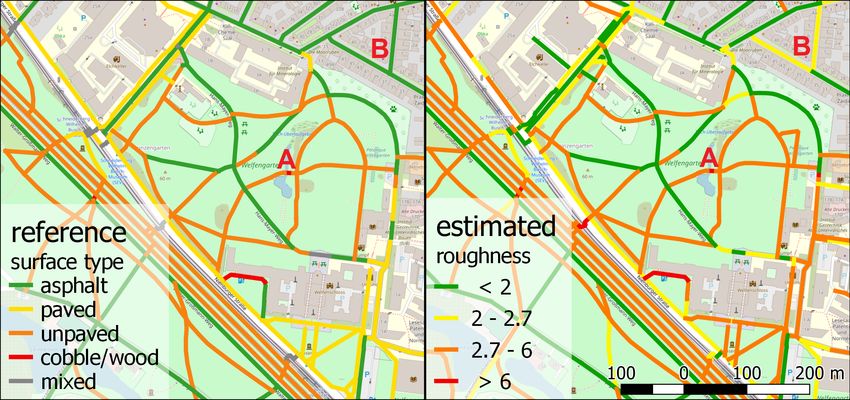
The available 1454 bike trips include 95337 segment passes and
Figure 2. Trajectory heat map as overview for Hanover network thus result in a corresponding amount of observations as input
exploration. (base map by Stamen Design, map data from for the adjustment. Those cover 17694 distinct segments, which
result – in combination with the number of trips – in 19148
OpenStreetMap)
unknown parameters to estimate.
About half of the trips were recorded by the authors alone (us- For an experimental evaluation, the adjustment approach of sec-
ing different bikes). This way we were able to reach quite a tion 2.3 was realized using the least squares function of the
good exploration rate of the center districts network (Figure 2), Python library Scipy (Virtanen et al., 2020) including the fol-
but also a basic coverage around. Due to the urban setting, a lowing cost function:
bias towards paved surfaces can be assumed. However, the au-
thors do not see this as a problem for the test scenario, since it 1 X
ρ fi (x)2
is a realistic application area for such an approach. In line with F (x) = ·
2 (4)
widespread behavior - but certainly reinforced by the desire to √
ρ(z) = 2 · 1+z−1
protect the smartphone from wetness - few trips in acute rain
are included, but this should not have a significant impact on where ρ(z) : soft-l1 loss function
roughness given the predominantly paved paths in urban areas. fi (x) : residuals
Only some very soft dirt paths in parks, etc., could be influ-
enced in their roughness by greater wetness, but this is not the Since many outliers are to be expected, a more robust soft-l1
purpose of this study. loss (smooth approximation of l1) is used instead of a standard
linear one. In contrast to the even more robust Cauchy loss,
3.1.2 Way network: To extract a georeferenced graph rep- experience has shown that this converges more reliably and was
resentation of the bikeable way network topology OSM (Open- therefore chosen as a compromise.
This contribution has been peer-reviewed. The double-blind peer-review was conducted on the basis of the full paper.
https://doi.org/10.5194/isprs-annals-V-4-2021-89-2021 | © Author(s) 2021. CC BY 4.0 License. 92ISPRS Annals of the Photogrammetry, Remote Sensing and Spatial Information Sciences, Volume V-4-2021
XXIV ISPRS Congress (2021 edition)
Figure 4. Plotted observation residuals (blue) with 5- and 95-percentiles (red).
4. RESULTS AND DISCUSSION the values of gravel paths diverge more, but their actual quality
also varies more.
For this study scenario after 156 iterations the adjustment con-
verged sufficiently. The change of the cost function (4) went Not only roughness is estimated, also trip (and thus implicitly
below the threshold of 10−8 , so no further significant changes user-bike setting) specific corrections. The resulting parameter
of the overall cost are assumed. The initial cost of 28813 was values of a selection (all are too confusing in a plot) of users
reduced to 17612. As a result, each segment is assigned an es- is plotted in combination with their trips over time in Figure
timated roughness value and each trip a correction factor. 7. Although the curves vary a lot, their different levels attract
attention: User 3, 24 and also 31 show up relatively high correc-
4.1 Resulting Residuals tion values most of the time, compared to others. Actually those
users rode sporty (track/racing) bikes with high tire pressures of
In Figure 4 the resulting residuals of all observations are plotted 6-8 bar. In contrast, users 10 and 32 went by classic city bikes,
as scatter. Although it looks quite noisy, the absolute median used between 2-3 bar and a more relaxed rider pose. Thus, even
of all values is 0.27. The lower 5-percentile is at a level of if they are noisy, the trip specific scale corrections show up to
-1.22 and the upper 95-percentile at 0.94, indicating a small adapt varying shock sensitivities. Based on this, future research
asymmetry. As an orientation, a difference of less than 1 is could reveal anomalous behavior like badly inflated tires.
subjectively rated by the authors as little perceptible in practice.
4.3 Multiply Observed Segments
In the case of very fine asphalt, this may already be caused by
several cracks or by a coarser asphalt composition. Figures 8 and 9 give a more detailed insight into specific way
segments. Beyond the overview of adjusted roughness paramet-
ers in Figure 6, they show two exemplary segments with mul-
tiple observations over time. The values of corrected roughness
observations give an impression of the measurement dispersion.
The variance of observations varies between different segments
and also coarse outliers can occur for different reasons. Due
to the very simple functional model, influences of the user-bike
system are assumed to be constant for a trip, so differing poses
Figure 5. Observation residuals plotted by related speed. over time or sequences of one/no hand riding are not handled
and can potentially distort the respective observations. A sim-
ilar effect will also result from incorrect map matching or miss-
Further, in Figure 5 the residuals can be visually checked to
ing way segments, which leads to wrong assignments of obser-
have no remaining systematic effects related to speed. The most
vations and segments. However, those issues should have no
common speed seems to be around 6 - 7 m/s, so about 21 - 25
major influence on the parameter estimation, because they only
km/h, coherent with a sporty bias of the users.
occur infrequently and thus for multiple observations the robust
loss function downgrades them.
4.2 Estimated Parameters
We refrain from presenting segment examples with perfectly
The estimated roughness parameters of the way segments are small deviations here and focus on two challenging examples
mapped exemplary for the area of the university park and il- with rather scattered and inhomogeneous roughness. Based on
lustrated in Figure 6 (right map). On the left are given the them, two observed inhomogeneity phenomena are differenti-
ways’ surface types as kind of reference. In general, segments ated and discussed in more detail, spatial and temporal inhomo-
of cobblestone or planks (with a roughness larger 6) are red, geneity:
badly paved and gravel paths (between 2.7 and 6) are colored
orange, smoothly paved ways are yellow (2 - 2.7) and plain 4.3.1 Spatially inhomogeneous segments occur with very
asphalt (roughness smaller 2) is green. Even a small wood scattered or reoccurring outlier roughness samples over the full
planked bride over a small pond in the park (A) is represented time period. Possible reasons are very inhomogeneous way
(reasonably) as a quite coarse part. Most asphalted main ways profiles or inconsistencies at road intersections. But also un-
and streets show similar values less than 2, but those in a bad modeled parallel tracks or incorrectly assigned segments can
condition (B) show similar roughness to paved parts. However, result in this.
This contribution has been peer-reviewed. The double-blind peer-review was conducted on the basis of the full paper.
https://doi.org/10.5194/isprs-annals-V-4-2021-89-2021 | © Author(s) 2021. CC BY 4.0 License. 93ISPRS Annals of the Photogrammetry, Remote Sensing and Spatial Information Sciences, Volume V-4-2021
XXIV ISPRS Congress (2021 edition)
Figure 6. To give an example of the results, way segments in and around the university park are colored by their surface type (left) and
by the estimated roughness value (right). They are ordered by smoothness and colored from green (asphalt - smooth) to red
(cobblestone/wood planks - rough). For an easy comparison the estimated roughness values are also grouped into four related classes.
(base map and data from OpenStreetMap)
Figure 7. Plot of estimated trip parameters over time. They are
colored by user and include the median as dashed line. User 3,
24 and 31 rode sporty track bikes with high tire pressures and
users 10 and 32 city bikes.
An example for this type of inhomogeneity is given in Figure 8.
Most of the samples are located on a level around the actually Figure 8. Plot of adjusted roughness observations over time for
estimated roughness (dashed green line). Beside those, some an exemplary street segment. The coarse outliers are assumed to
outliers from different users with higher values of about 3-5 are result from incorrectly assigned observations, actually belonging
occurring infrequently over the time. The segment is one of to the parallel sidewalk.
the roadways of Schneiderberg street shown in Figure 3 with
separated (but optional to use) bike paths on both sides. Thus ing alternative ways to be added to the network model. This
those outliers can be assumed to result from wrong matches will be investigated in future work.
due to the small margin between both similar courses. Those
samples indicating a substantial higher level of roughness were 4.3.2 Temporally inhomogeneous way segments actually
actually sensed on the poorly paved bike and foot path next changed their roughness over time. This might happen in both
to the smoothly asphalted roadway and are only linked to the directions, lower e.g. due to a reconstruction, or higher e.g. due
roadway segment because of an inaccurate trajectory and thus to additional damages or seasonal effects like massive autumnal
wrong map matching. However, the estimation of the actual leaves and branches which can fall on the ground.
roughness adapts robustly to the majority of the observations,
thus a relevant influence is not expected, but of course this find- An example of this type is given in Figure 9. In the first half of
ing could be used to correct the matching. the plot the observations scatter around the estimated rough-
ness (dashed green line), but after a gap between April and
Similar patterns might occur when alternative/parallel paths are June 2020 further observations are located on a significantly
missing in the underlying road network. In those cases, occa- smoother (lower roughness) level. A plausible reason for this
sionally reoccurring coarse outliers are a hint on actually exist- effect is a road reconstruction of this segment’s asphalt, which
This contribution has been peer-reviewed. The double-blind peer-review was conducted on the basis of the full paper.
https://doi.org/10.5194/isprs-annals-V-4-2021-89-2021 | © Author(s) 2021. CC BY 4.0 License. 94ISPRS Annals of the Photogrammetry, Remote Sensing and Spatial Information Sciences, Volume V-4-2021
XXIV ISPRS Congress (2021 edition)
algorithm correctly identifies July 15th as change point (based
on the minimum within class variance, depicted in Figure 10,
lower part). As an advantage of this method, there is no need
for assumptions about the change point. Further, no threshold
parameters need to be given.
5. CONCLUSION
This paper addresses the problem of integrating measurements
of roughness from diverse bikes and users into a jointly scaled
representation by applying a least-squares adjustment. A case
study is carried out to test the presented approach with real-
world floating smartphone data.
The underling way network was extracted from OpenStreetMap
and the sensor data was acquired with standard smartphones
running a special logging app. Participant just needed to attach
Figure 9. Plot of adjusted roughness observations over time for a phone to their bike and collected trajectory and acceleration
an exemplary street segment. The temporal discontinuity results data while riding their trips.
from a new asphalt surface in May 2020, before it had several
cracks. The collected trajectory data is automatically map matched to
the way segments. Then, the vertical acceleration signal of
each segment pass is transformed into a robust roughness in-
dex. Those are used as observation input for a least-squares
adjustment, to estimate trip-wise scaling factors and a corrected
roughness parameter for each segment. Alongside the robustly
estimated roughness parameters for each segment, also a way’s
change over time can be analyzed across varying bike-user set-
tings. In addition, a method for automatic detection of abrupt
changes (e.g. due to reconstruction) in the surface quality is
suggested and applied to an exemplary street.
Even if the functional and stochastic models are quite basic, the
results and conclusions of the case study already show sufficient
performance for the intended purposes. Thus, this is a prom-
ising approach to collectively evaluate crowd-sourced ride dy-
namics using commonly available smartphones. Despite the re-
lated inhomogeneities and without explicit knowledge of the re-
spective settings, the information can be supplemented to form
a unified view of the ways surface roughness. With sufficient
dissemination, spatial and temporal coverage could be achieved
in a way that would not be possible with individual specialized
measurement systems.
Figure 10. Example of an automatic change detection via Otsu Resulting outputs like a roughness map of the way and street
segmentation in segment of Figure 9. graph can be used as weight factor in comfort sensitive bike
routing services. Besides individual mobility, efficient bicycle
navigation is also gaining importance in commercial traffic, es-
took place around May 2020. The asphalt surface before was pecially in the area of increasingly bicycle-based urban logist-
in a bad condition with several cracks and potholes. This way, ics (e.g. food and parcel delivery services). Further, pain points
affected segments can be split into two (or more) virtual ones, in the network can not only be bypassed via such a routing,
representing it before and after the break point. Alternatively, but also could be identified in quasi-real time for future infra-
even more straight forward, all observations before the break structure maintenance and planning. Further, a conceivable re-
point can be filtered out and ignored in a future adjustment to search option would be to use the knowledge gained about the
represent only the latest network state. This, however, presumes surface conditions for an additional similarity measure in map
that such break points are identified automatically. matching. In this way, despite their spatial proximity, paral-
lel roads and bike paths could be better differentiated based on
Based on the discussed example in Figure 9 a first test for an their roughness.
automatic change (or break point) detection for a temporally
inhomogeneous segment was applied. Otsu’s method (Otsu, Besides those findings, there are open issues, which should be
1979), originally suggested for basic fore- and background seg- addressed and included in future works into the modular and
mentation in image analysis, was adapted to segment the two flexible process chain. One of those is to introduce reference
major roughness level over time. The result plotted in Figure 10 values for several segments into the adjustment. Such refer-
nicely shows the roughness of about 2.8 before and 1.1 after the ence values could be determined using a theoretical analysis of
asphalt changes sometime between March and July 2020. The rough surfaces. An alternative is to use another data source, e.g.
This contribution has been peer-reviewed. The double-blind peer-review was conducted on the basis of the full paper.
https://doi.org/10.5194/isprs-annals-V-4-2021-89-2021 | © Author(s) 2021. CC BY 4.0 License. 95ISPRS Annals of the Photogrammetry, Remote Sensing and Spatial Information Sciences, Volume V-4-2021
XXIV ISPRS Congress (2021 edition)
LiDAR point clouds, to analyze the surface and derive a proxy Karakaya, A.-S., Hasenburg, J., Bermbach, D., 2020.
for the roughness. In this way, there would be an absolute refer- SimRa: Using crowdsourcing to identify near miss hot-
ence and also regions (e.g. different cities) which are not linked spots in bicycle traffic. Pervasive and Mobile Computing,
by joint trips, could be leveled in a common scale and thus be 67, 101197. http://www.sciencedirect.com/science/
comparable. Also a more detailed accuracy investigation for article/pii/S157411922030064X.
observations and parameters and a more refined integration of
Kastl, D., Nagase, K., Obe, R., Vergara, V., Sharma, A., Pavie,
stochastic information would be supported by absolute and su-
A., Patrushev, A., Wendt, D., Anderson, J., Kumar, J. K.,
perior reference observations. Gained insights would also facil-
de Sousa, L., Agarwal, S., 2017. osm2pgrouting v2.3.1. https:
itate a refinement (and extension) of the functional model.
//pgrouting.org/docs/tools/osm2pgrouting.html.
In summary, the calibration approach presented here for surface komoot GmbH, 2021. Komoot. https://www.komoot.com.
roughness determination of bike paths is a relevant progres-
sion from recent bike specific approaches. The process chain Leys, C., Ley, C., Klein, O., Bernard, P., Licata, L.,
enables to analyze crowd-sourced data without further explicit 2013. Detecting outliers: Do not use standard deviation
knowledge about the user and bike system. Only based on ac- around the mean, use absolute deviation around the me-
celeration (and location) data, the differently scaled trips can be dian. Journal of Experimental Social Psychology, 49(4), 764 -
fit on each other via shared way segments. 766. http://www.sciencedirect.com/science/article/
pii/S0022103113000668.
ACKNOWLEDGEMENTS Luhmann, T., Robson, S., Kyle, S., Boehm, J., 2013. Close-
Range Photogrammetry and 3D Imaging. Walter de Gruyter.
This work is partially funded by the BMBF Germany projects McCarthy, O. T., Caulfield, B., Deenihan, G., 2016. Evaluating
USEfUL and USEfUL XT (grants 03SF0547B & 03SF0609C), the quality of inter-urban cycleways. Case Studies on Transport
as well as supported by the DFG GRK 1931 SocialCars. The Policy, 4(2), 96–103.
authors also thank the volunteers who contributed to the data
collection and the reviewers for their valid and helpful feed- Newson, P., Krumm, J., 2009. Hidden Markov Map Matching
back. Through Noise and Sparseness. Proceedings of the 17th ACM
SIGSPATIAL International Conference on Advances in Geo-
graphic Information Systems, GIS ’09, ACM, New York, NY,
REFERENCES USA, 336–343. event-place: Seattle, Washington.
OpenStreetMap contributors, 2020. Data dump retrieved from
Bike Citizens Mobile Solutions GmbH, 2021. Bike citizens.
https://planet.osm.org . https://www.openstreetmap.org.
https://www.bikecitizens.net.
Otsu, N., 1979. A Threshold Selection Method from Gray-
Bı́l, M., Andrášik, R., Kubec̆ek, J., 2015. How comfortable are Level Histograms. IEEE Transactions on Systems, Man, and
your cycling tracks? A new method for objective bicycle vibra- Cybernetics, 9(1), 62-66.
tion measurement. Transportation Research Part C: Emerging
Technologies, 56, 415–425. Stinson, M. A., Bhat, C. R., 2003. Commuter Bicyc-
list Route Choice: Analysis Using a Stated Prefer-
Bovy, P. H. L., Bradley, M. A., 1985. Route Choice Analyzed ence Survey. Transportation Research Record: Journal
with Stated-Preference Approaches. Transportation Research of the Transportation Research Board, 1828(1).
Record, 1037, 10. https://journals.sagepub.com/doi/abs/10.3141/1828-13.
Brauer, A., Mäkinen, V., Oksanen, J., 2021. Characteriz- van Overdijk, R.P.J., 2016. The influence of comfort aspects on
ing cycling traffic fluency using big mobile activity track- route- and mode-choice decisions of cyclists in the netherlands:
ing data. Computers, Environment and Urban Systems, an approach to improve bicycle transportation planning in prac-
85, 101553. http://www.sciencedirect.com/science/ tice. Master’s thesis, Eindhoven University of Technology.
article/pii/S0198971520302866.
Virtanen, P., Gommers, R., Oliphant, T. E., Haberland, M.,
Broach, J., Dill, J., Gliebe, J., 2012. Where do cyclists ride? Reddy, T., Cournapeau, D., Burovski, E., Peterson, P., Weck-
A route choice model developed with revealed preference GPS esser, W., Bright, J., van der Walt, S. J., Brett, M., Wilson,
data. Transportation Research Part A: Policy and Practice, J., Millman, K. J., Mayorov, N., Nelson, A. R. J., Jones, E.,
46(10), 1730–1740. Kern, R., Larson, E., Carey, C. J., Polat, İ., Feng, Y., Moore,
E. W., VanderPlas, J., Laxalde, D., Perktold, J., Cimrman, R.,
Dane, G., Feng, T., Luub, F., Arentze, T., 2019. Route Choice Henriksen, I., Quintero, E. A., Harris, C. R., Archibald, A. M.,
Decisions of E-bike Users: Analysis of GPS Tracking Data in Ribeiro, A. H., Pedregosa, F., van Mulbregt, P., SciPy 1.0 Con-
the Netherlands. P. Kyriakidis, D. Hadjimitsis, D. Skarlatos, tributors, 2020. SciPy 1.0: Fundamental Algorithms for Sci-
A. Mansourian (eds), Geospatial Technologies for Local and entific Computing in Python. Nature Methods, 17, 261–272. ht-
Regional Development, Lecture Notes in Geoinformation and tps://rdcu.be/b08Wh.
Cartography, Springer International Publishing, Cham, 109–
Wage, O., Feuerhake, U., Koetsier, C., Ponick, A., Schild,
124.
N., Beening, T., Dare, S., 2020. RIDE VIBRATIONS: TO-
Dawkins, J., Bishop, R., Powell, B., Bevly, D., 2011. Investiga- WARDS COMFORT-BASED BICYCLE NAVIGATION. IS-
tion of pavement maintenance applications of intellidrivesm (fi- PRS - International Archives of the Photogrammetry, Re-
nal report): Implementation and deployment factors for vehicle mote Sensing and Spatial Information Sciences, XLIII-
probe-based pavement maintenance (pbpm). Technical report, B4-2020, 367–373. https://www.int-arch-photogramm-remote-
Auburn University. sens-spatial-inf-sci.net/XLIII-B4-2020/367/2020/.
This contribution has been peer-reviewed. The double-blind peer-review was conducted on the basis of the full paper.
https://doi.org/10.5194/isprs-annals-V-4-2021-89-2021 | © Author(s) 2021. CC BY 4.0 License. 96You can also read