Muon radiography to visualise individual fuel rods in sealed casks - EPJ N
←
→
Page content transcription
If your browser does not render page correctly, please read the page content below
EPJ Nuclear Sci. Technol. 7, 12 (2021)                                                                                              Nuclear
                                                                                                                                    Sciences
 c T. Braunroth et al., Published by EDP Sciences, 2021                                                                             & Technologies
https://doi.org/10.1051/epjn/2021010
                                                                                                                          Available online at:
                                                                                                                         https://www.epj-n.org

    REGULAR ARTICLE

Muon radiography to visualise individual fuel rods in sealed
casks
Thomas Braunroth 1, * , Nadine Berner 2 , Florian Rowold 3 , Marc Péridis 2 , and Maik Stuke 4
1
    GRS   gGmbH, Schwertnergasse 1, 50667 Cologne, Germany
2
    GRS   gGmbH, Boltzmannstr. 14, 85748 Garching, Germany
3
    GRS   gGmbH, Kurfürstendamm 200, 10719 Berlin, Germany
4
    BGZ   mbH, Dammstraße, 84051 Essenbach, Germany

             Received: 26 February 2021 / Received in final form: 4 May 2021 / Accepted: 11 May 2021

             Abstract. Cosmic-ray muons can be used for the non-destructive imaging of spent nuclear fuel in sealed dry
             storage casks. The scattering data of the muons after traversing provides information on the thereby penetrated
             materials. Based on these properties, we investigate and discuss the theoretical feasibility of detecting single
             missing fuel rods in a sealed cask for the first time. We perform simulations of a vertically standing generic
             cask model loaded with fuel assemblies from a pressurized water reactor and muon detectors placed above and
             below the cask. By analysing the scattering angles and applying a significance ratio based on the Kolmogorov-
             Smirnov test statistic we conclude that missing rods can be reliably identified in a reasonable measuring time
             period depending on their position in the assembly and cask, and on the angular acceptance criterion of the
             primary, incoming muons.

1 Introduction                                                              several orders of magnitude and have a mean momentum
                                                                            of approximately 4 GeV/c [4]. For muons with an absolute
The operation of nuclear power plants generates high-level                  momentum above 1 GeV/c the integral vertical intensity
radioactive wastes which need to be stored and disposed                     IV is approximately 70 m−2 s−1 sr−1 [5,6] and the decrease
of. A well-established part of nuclear waste management                     of the flux intensity scales approximately with cos(θ), with
is the dry storage of used fuel assemblies in designated                    θ being the angle with respect to the vertical [4]. In exper-
casks. Depending on the availability of a final repository,                 imental physics, a value of IV ≈ 1 cm−2 min−1 has been
the fuel assemblies might remain inside the casks placed                    established for working with horizontal detectors.
in interim storage facilities for decades. The casks are                       Alvarez and colleagues were one of the first to use
designed to enclose the high-level radioactive waste and                    muons for non-invasive imaging and published their land-
separate it from the biosphere.                                             mark paper on the search for hidden chambers in the
   Inspecting the interior of a storage cask directly would                 pyramids of Giza in 1970 [7]. These first studies were
require an opening of the cask, a difficult task due to                     based on the measurement of the attenuation of the cos-
the radiation. So far, conventional radiography using neu-                  mic muon flux and provided two-dimensional projection
trons or photons could not be applied successfully, partly                  images (muon radiography). Since then, muon radiogra-
due to the rich scattering history of traversing particles                  phy has been used in various fields such as the study of
as a direct result of the dimensions of the storage cask                    volcanoes [8], geological applications [9], the identifica-
[1]. Other methods such as three-dimensional temperature                    tion of cavities in archaeology [10] as well as in industrial
field measurements or antineutrino monitoring [2] require                   applications [11].
a detailed knowledge of the fuel history or are not suit-                      In 2003, a Los Alamos research group proposed using
able for the assessment of individual storage casks. Cosmic                 the scattering angle of the outgoing muons as the basic
muons, created directly or indirectly in the atmosphere by                  information for imaging [12]. This approach requires the
the interaction of cosmic radiation with particles, have                    measurement of the incoming as well as the outgoing
been also used for imaging purposes (muography) [3].                        trajectories of the muons and allows to obtain three-
These muons and anti-muons (muons in the following)                         dimensional images (muon tomography) of volumes not
are characterized by a broad energy spectrum spanning                       exceeding tens of meters. This technique has already been
                                                                            used in various fields, such as nuclear control [13], trans-
*   e-mail: thomas.braunroth@grs.de                                         port control [14] and the monitoring of historical buildings

This is an Open Access article distributed under the terms of the Creative Commons Attribution License (https://creativecommons.org/licenses/by/4.0),
             which permits unrestricted use, distribution, and reproduction in any medium, provided the original work is properly cited.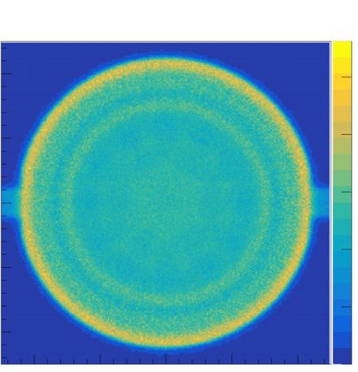
2                                   T. Braunroth et al.: EPJ Nuclear Sci. Technol. 7, 12 (2021)

[15]. In addition to experimental studies, Monte-Carlo         Does the significance depend on the relative position of the
simulations play an important role in muon imaging,            considered fuel rod within the fuel assembly and is the sig-
e.g. in terms of feasibility studies or with respect to the    nificance dependent on the number of considered events?
detector design.                                                  This contribution is structured as follows: in Section 2
   The application of muography for the purpose of non-        we provide a detailed description of the simulation tool as
invasive control and monitoring of the interior of dry         well as the investigated geometry. Moreover, we describe
storage casks has gained an increasing interest and fos-       the data processing and aspects related to the validation
tered experimental and simulation studies. Besides the         of the simulation. Section 3 features the analysis and dis-
fundamental suitability of muography for this purpose,         cussion. We address two levels of detail concentrating on
these efforts also addressed methodological and time           the recognition of (missing) fuel assemblies and individual
requirements. Durham et al. [16] applied muon-scattering       fuel rods. This is followed by a summary and conclusion
radiography to a Westinghouse MC-10 cask and showed            in Section 4. We end with a short outlook in Section 5.
experimentally that cosmic muons can indeed be used to
determine if spent fuel assemblies are missing without the
need to open the cask. A number of simulation studies
                                                               2 Simulation and data processing
were performed using two planar tracking detectors placed
on opposite sides of an object, each focusing on different     Simulations were performed with a dedicated tool based
aspects, for example: Jonkmans et al. [17] investigated the    on the Monte-Carlo toolkit Geant4 [23–25]. Geant4 allows
capabilities of muons to image the contents of shielded        simulating the passage of particles through matter and
containers to detect enclosed nuclear materials with high-     has been used for numerous applications, including high
Z. Clarkson et al. [18] performed Geant4 simulations           energy physics, nuclear physics, accelerator physics and
of a scintillating-fibre tracker for tomographic scans of      others.
legacy nuclear waste containers. Chatzidakis [19] applied         In this section we describe the key aspects of the tool,
a Bayesian approach to monitor sealed dry casks to infer       i.e. the geometry (Sect. 2.1), the treatment of primary
on the amount of spent nuclear fuel and to investigate         particle properties (Sect. 2.2), aspects related to physics
the limitiations of this approach. Using the attenuation       and tracking (Sect. 2.3) as well as optimization strategies
and scattering characteristics of the muons derived from       (Sect. 2.4) to reduce the computational time.
Geant4 simulations, Ambrosino et al. [20] found that a            The tool was compiled against v10.06.p2 of Geant4 and
10 cm3 Uranium block inside a concrete structure could         allows using multithreading. The results are written event-
be identified after a one-month period of measurement.         by-event into ROOT [26,27] container files, which allows
Poulsen et al. [21] were the first to apply filtered back-     performing post-processing in a flexible manner. Finally,
projection algorithms to muon tomography imaging of dry        Section 2.5 discusses the validation of the code by compar-
storage casks using simulated data and could show that         ing simulated and tabulated (or empirically established)
this technique can be applied to the detection of missing      energy losses and angular straggling for different target
fuel assemblies. In a more recent work, Poulsen et al. [22]    materials and projectile energies.
used the experimental data of reference [16] for a numer-
ical study using Geant4 to distinguish different loads of      2.1 Geometry
a cask. The study indicates that a one-week muon mea-
surement for the given experimental setup is sufficient to     2.1.1 Generic cask
detect a missing fuel assembly or to identify a dummy          The key component of the geometry is a generic cask
assembly made out of iron or lead.                             model (referred to as generic model in the following) which
   With respect to the resolving power, both experimental      mimics the features of the CASTOR R V/19 cask [28], e.g.
and simulation studies have been focused on the level of       in terms of major components, dimensions, materials and
fuel assemblies so far. In addition, the majority of stud-     masses. The CASTOR R V/19 cask is used for transport
ies are based on a transversal configuration, where the        as well as storage purposes and is designed to carry up to
detectors are placed on the sides of the cask.                 19 fuel assemblies from pressurized water reactors (PWR).
   In this study, we use Monte-Carlo simulations to inves-     All information on geometries and materials specifying the
tigate a longitudinal configuration, with the detectors        generic model was derived from public available sources
placed above and below the cask. We will investigate           such as references [28,29].
if muography allows detecting individual missing fuel             A visualisation of the generic model was generated with
rods. To unravel insights independent of reconstruction        the Geant4 OpenGL interface and is depicted in Figure 1.
algorithms, this work will focus on radiographic images        The individual components of the generic model can be
based on transmission ratios as well as scattering-angle       identified in the exploded view shown in Figure 2.
information.                                                      A comparison of some key properties of the generic
   The guiding questions of this work are as follows: is it    model on the one hand and the CASTOR R V/19 cask
possible to even detect individual missing fuel rods with      on the other hand can be found in Table 1 and highlights
muon radiography? If so, are there any constraints or          the mutual similarities.
requirements with respect to the experimental setup and           Each of the 19 fuel compartments can be occupied with
how much time does a measurement require? What can be          one (modelled) fuel assembly. Each modelled fuel assembly
used as a significance measure to detect a missing fuel rod?   comprises top- and bottom-nozzle, fuel rods as well as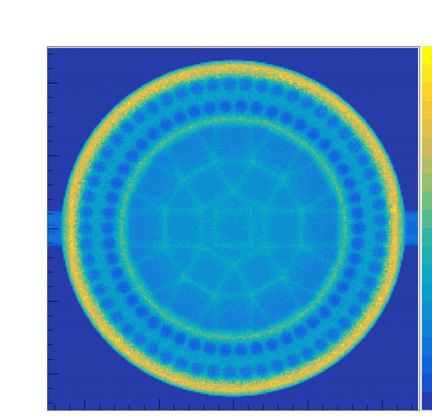
T. Braunroth et al.: EPJ Nuclear Sci. Technol. 7, 12 (2021)                                      3

                                                                   Fig. 2. Exploded view of the generic model showing its indi-
                                                                   vidual components: monolithic body (1), basket with 19 fuel
                                                                   compartments (2), trunnions (3), primary lid (4), polyethylene
                                                                   plate (5), secondary lid (6), protection plate (7), inner moder-
                                                                   ator rods and plugs (8), outer moderator rods and plugs (9),
                                                                   polyethylene plate (10), base plate (11) and a representative fuel
                                                                   assembly (12). See text for details.

                                                                   Table 1. Comparison of key dimensions between the
                                                                   generic model and the CASTOR R V/19 cask (in storage
                                                                   configuration).
                                                                    Property             Generic Model CASTOR R V/19 [28]
                                                                    Overall height       594 cm             594 cm
                                                                    Outer diameter       244 cm             244 cm
                                                                    Cavity height        502.5 cm           503 cm
                                                                    Cavity diameter      148 cm             148 cm

Fig. 1. Visualisation of the generic model and its upward ori-
entation within the present work. The coordinate system as it
is used in this study is provided in the lower right corner. The
origin of the coordinate system coincides with the center posi-
tion of the bottom part of the model. The red and green areas
above and below the model indicate the incoming and outgoing
detectors.

control rods. The fuel rods consist of nuclear fuel (UO2 )
and cladding tubes (Zirconium alloy). A complete 18x18-
24 fuel assembly consists of 300 fuel rods and 24 control
rods. The arrangement of fuel and control rods within a
                                                                   Fig. 3. Left: top-view on the arrangement of fuel rods (yellow),
complete fuel assembly is shown in Figure 3. The modelled          cladding tubes (green) as well as control rods (blue) in case of
top and base components of the assembly are simplified.            a complete fuel assembly. Each element can be specified unam-
They are assumed to be box-like, with heights chosen to            biguously based on its slot position given by xid , yid . Right: same
comply with real masses. Basic properties related to the           as left figure, but several elements along the diagonal are miss-
modelled fuel assemblies are summarized in Table 2.                ing (xid /yid = 1, 5, 9). This configuration is investigated in more
   All parts of the Geant4 model were derived from basic           detail in Section 3.2.
Geant4 solid objects and refined with Boolean opera-
tions. Each component can be switched on and off by a
                                                                   2.1.2 Box-like object
command-based user interface, which easily allows per-
forming simulations for different target geometries. In            Instead of the generic model, it is possible to generate a
addition, it is possible to remove arbitrary components            box-like object, whose basic properties – i.e. dimensions,
from a fuel assembly, e.g. specific fuel rods at specific          placement and material – can be specified individu-
slot positions. This allows, among others, for investigat-         ally for each simulation run. All interactions within this
ing the contribution of specific fuel rods to radiographic         box are recorded within ROOT container files, which is
(or tomographic) images in more detail.                            particularly useful for validation purposes.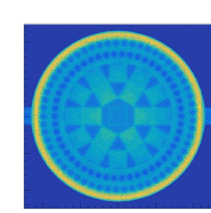
4                                            T. Braunroth et al.: EPJ Nuclear Sci. Technol. 7, 12 (2021)

Table 2. Properties of the modelled fuel assemblies.                          i.e. particle type (muon (µ− ) or anti-muon (µ+ )), ini-
     Value/Parameter              Property                                    tial momentum information (pµk , θk , ϕk ) as well as initial
                                                                              position information (xk , yk ). Details are described in the
        Material – Head and base             Stainless Steel
                                                                              following.
        Material – Cladding                  Zirconium Alloy
        Material – Fuel                      Uranium Dioxide
        Material – control rods              Zirconium Alloy                  2.2.1 Particle type
        Length – fuel rod                    4407 mm
        Length – active length               3900 mm                          All primaries are muons or anti-muons, assuming a charge
        Number of control rods               24                               ratio µ+ /µ− equal to 1.28 [30]. The particle type for the
        Number of fuel rods                  300                              event k is determined assuming U[0; 2.28] - if the generated
        Total weight                         845 kg                           random number is smaller than (or equal to) 1.28, the
                                                                              generated primary for this event will be an anti-muon
                                                                              (µ+ ), otherwise it will be a muon (µ− ).

2.1.3 Coordinate system
                                                                              2.2.2 Initial particle momentum
 The z-axis coincides with the symmetry axis of the generic
 model and is oriented upwards, i.e. its orientation is                       The description of the initial muon momentum is based
 selected so that the z-coordinate of the model’s top is                      on an empirical and parametric approach [31], according
 larger than the z-coordinate of its bottom, ztop > zbottom .                 to which the muon intensity at any given momentum and
 The x and y axis are orientated in such a way that                           angle to the vertical intensity IV is given by
 the (x, y, z)-coordinate system generates a right-handed
 euclidean space. The orientation of the individual axes is                                I(pµ , θ) = cos3 (θ) · IV (pµ · cos(θ)).                     (1)
 indicated in Figure 1. The angle θ reflects the angle of a
 given vector ~r and the inverted z-axis. Using this conven-                  Here, IV is given by the Bugaev parametrisation [32]:
 tion, a muon from the zenith is characterized by θ = 0◦ .                                       −(c2 +c3 ·log10 (pµ )+c4 ·log210 (pµ )+c5 ·log310 (pµ ))
 The angle ϕ is the angle between the projection of a vector                    IV (pµ ) = c1 · pµ                                  .
~r onto the (x, y)-plane and êx .                                                                                                  (2)
                                                                              The parameters c1 to c5 were determined in reference [31]
                                                                              by a fitting approach and are quantified as:
2.1.4 Detectors
Detector systems are mimicked by two rectangular detec-                                                   c1   = 0.00253
tor planes (vanishing thickness, area of (3 × 3) m2 ), whose                                              c2   = 0.2455
normal vectors are parallel to êz . The detector plane
                                                                                                          c3   = 1.288
placed above the generic model is called incoming detector
whereas the detector plane placed below the generic model                                                 c4   = −0.2555
is called outgoing detector. The gap between the detector                                                 c5   = 0.0209.
surface and the top (or the bottom) of the generic cask is
≈ 10 cm. Muons traversing these planes are tracked and                        Due to the lack of a suitable random number generator
key information is determined, see Section 2.3.                               to directly address the associated probability distribution
   This approach gives access to at least as many prop-                       in Geant4, the analytical description is discretized in a
erties as a real detection system for muon tomography                         two-dimensional pattern as follows.
may provide. Since the simulation allows determining all                         Firstly, the polar component of the angular spectrum
properties precisely on an event-by-event base, it bene-                      represented by θin , ranging from θmin = 0◦ to an upper
fits from an infinite resolving power.1 In this regard, it                    limit of θmax = 25◦ , is split into n bins bθ,i (i = 1, . . . , n).
provides a best-case scenario and can be considered as                        The quoted upper limit of 25◦ limits the contribution of
a first important theoretical step towards substantiated                      trajectories that do not cross the full longitudinal length
feasibility studies.                                                          of the cask. All bθ,i span over identical angular ranges. For
                                                                              each angular bin bθ,i , the lower and upper limits are then
2.2 Primary particles                                                         given by θill [◦ ] = 25 (i−1)
                                                                                                        n   and θiul [◦ ] = 25 ni .
                                                                                 The function Ii (pµ , θi ), for i = 1, . . . , n, can then be
Primaries are generated by a user-defined class based on                      associated to each of these bins of the angular spectrum,
the G4VUserPrimaryGeneratorAction class provided by                           where θi is the arithmetic mean angle of the specific bin.
Geant4.                                                                       These assigned functions Ii are then integrated numeri-
   The Monte-Carlo approach is realized by using uni-                         cally within the kinetic energy range of T ∈ [1 GeV; 1 TeV].
form random number generators with limits a, b (U[a; b])                      The calculated integrals quantify the relative weights wi
to determine for each event k the particle properties,                        for each of the angular bins bθ,i :
    1
    In principle, the present approach allows to include resolution effects                          Z   pµ (T =1 TeV)
in the post-processing without the need to repeat time-consuming                            wi =                         dp0µ Ii (p0µ , θi ).           (3)
simulations.                                                                                         pµ (T =1 GeV)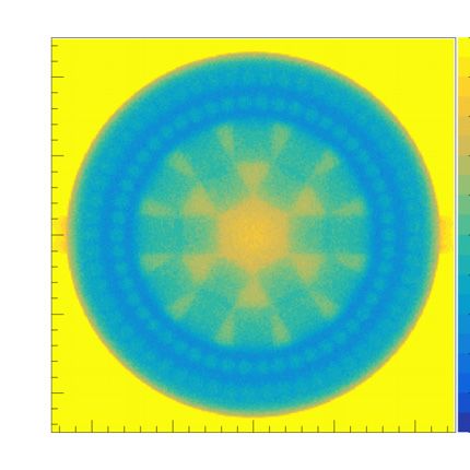
T. Braunroth et al.: EPJ Nuclear Sci. Technol. 7, 12 (2021)                          5

                                                                                respectively. The associated limits can be specified in the
                                                                                input file of the simulation.

                                                                                2.3 Physics and tracking
                                                                                This code uses the modular physics list FTFP BERT
                                                                                implemented in Geant4, which is recommended by the
                                                                                Geant4 developers for high-energy physics.
                                                                                   The incoming and outgoing detector volumes are linked
                                                                                to a dedicated tracking class. This allows tracking and
Fig. 4. Sample distributions of the initial angle θin (left) and of             storing information on the particle properties needed
the absolute muon momentum p (right) as determined with the                     for the post processing to generate radiographic (or
incoming detector. The red curve shown in the left spectrum is                  tomographic) images.
proportional to cos2 (θ), while the red curve shown in the right
spectrum is proportional to equation (1) with θ = 12.5◦ .
                                                                                2.4 Cutting conditions to reduce computational time
Information on   θill ,   θiul
                             and wi are stored in a dedicated text              Muons may interact with the materials of the generic
file that
        P    is used   as an  input parameter to the simulation.                model according to the chosen physics list in various
U[0, i wi ] uses these weights wi to determine for each                         ways. Some of these interactions are irrelevant to the
event k the proper angular bin bθ,k . In a next step, the                       present work. For example, some interactions may gener-
proper polar angle θk for the present event k is determined                     ate secondary particles – e.g. photons or neutrons – whose
using U[θkll ; θkul ]. The azimuthal angle ϕk is determined for                 tracking consumes computational time without any ben-
each event k using U[−π; π].                                                    efits or consequences to the generated images. To avoid
   Secondly, the absolute momentum spectra are treated                          an unnecessary increase of the computational time, the
comparably. The momentum axis from pµ (T = 1 GeV)                               trajectories of such secondary particles are annihilated at
to pµ (T = 1 TeV) is discretized into m bins bpµ ,j (j =                        the end of their first steps. It must be stressed that this
1, . . . , m) with increasing bin sizes. Each bin bpµ ,j is                     does not concern the possible interactions of muons with
characterized by the following integral:                                        matter - all interactions which may lead to such secondary
                                                                                particles still take place.
                                 Z   pul
                                      µ,j                                          In addition and as already described in Section 2.2,
                  vi,j =                    dp0µ Ii (p0µ , θi ).          (4)   the muon properties – with respect to the angle θ and
                                 pllµ,j
                                                                                kinetic energy T – were cut to limit the simulation of
                                                                                muon trajectories that are not useful for an analysis based
Here, pllµ,j and pul
                  µ,j denote the lower and upper limits of                      on a two-detector setup. Finally, all muon trajectories are
the bin bpµ ,j .
                                                                                annihilated at the exit of the outgoing detector.
   For each angular bin bθ,i , values for pllµ,j , pul
                                                     µ,j and
vi,j are stored in dedicated text files which are used as
mandatory
        P input information for the simulation code.                            2.5 Validation
   U[0; j vi,j ] uses these weights vi,j to determine for
each event k the proper momentum bin bpµ ,k . Finally, the                      This section discusses the validation of two key aspects
proper pµ,k is determined using U[pllµ,k ; pul                                  with respect to muon imaging. The first aspect deals with
                                            µ,k ]. Within the
                                                                                the energy loss of muons in matter and is discussed in
present work, all numerical integrations were performed
                                                                                Section 2.5.1. The second aspect deals with the angular
with GNU Octave [33].
                                                                                scattering of muons after traversing matter with a known
   Figure 4 shows histograms of the simulated angular and
                                                                                thickness, see Section 2.5.2. In both cases, the referenced
momentum distributions for θmin = 0◦ , θmax = 25◦ , n = 10
                                                                                thickness was specified to 1 mm.
and m = 172.
   In addition to this distribution-based approach
described above, the tool also allows performing simu-                          2.5.1 Energy loss of Muons in various target materials
lations with mono-energetic and mono-directional muons.
                                                                                In this section, we compare simulated energy losses of
                                                                                muons in relevant target materials – uranium dioxide,
                                                                                polyethylene, stainless steel, ductile iron and zirconium
2.2.3 Initial particle position
                                                                                alloy – to tabulated (or calculated) values of the mean
The initial positions of the muons are selected as fol-                         differential energy loss [34,35].
lows. The z-coordinate is a fixed value and selected so                            The quoted references provide only for two of the listed
that it is ensured that the muon is created just above the                      compound materials – uranium dioxide and polyethylene –
incoming detector. The x- and y-coordinates are selected                        tabulated values. Hence, reference values were calculated
from uniform distributions covering ranges from xmin                            for the other compounds – stainless steel, ductile iron and
to xmax (U[xmin ; xmax ]) and ymin to ymax (U[ymin ; ymax ]),                   zirconium alloy – according to Bragg’s Rule of Stopping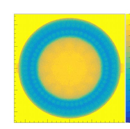
6                                   T. Braunroth et al.: EPJ Nuclear Sci. Technol. 7, 12 (2021)

Power Additivity [36]:
                           n j · Aj
                    wj = P                               (5)
                           k n k · Ak
                   dE    X         dE
                       =    wj ·        .                (6)
                   dx    j
                                   dx j

Here, wj denotes the mass fraction of the material j,
dE/dx|j is the differential energy loss in the material j
and dE/dx describes the mean differential energy loss by
the muons in the compound material.
   Strictly speaking, the simulated energy losses per dis-
tance ∆E are not identical to differential energy losses.
To increase the comparability, we consider for both num-
bers a distance of 1 mm and cut the lower limit of the
considered kinetic energy range to ensure that the (simu-
lated) mean energy losses are smaller (or comparable) to
five percent of the kinetic energy T , i.e. ∆E . 0.05 T . The
upper limit of the kinetic energy range is set to T = 1 TeV
which equals the maximal kinetic energy of the considered
muon primaries in the present study.
   The number of simulated events was chosen in a way
that the relative uncertainties of the mean values ∆E
extracted from the simulated energy-spectra are below
2%. The only exception is given for polyethylene, for which
the limit is increased to 5%. In total, between 105 and
5 · 106 events were simulated for each kinetic energy and
each material. The results are shown in Figure 5.
   For the materials stainless steel, ductile iron and
zirconium alloy, the agreement between simulated and
tabulated values is very good and the majority of values
deviate by less than 2%. Few exceptions were found for
kinetic energies close to 1 GeV. It shall be mentioned that
due to the high ∆E dispersion at high projectile energies,
the mean values are quite sensitive to statistical outliers.
   The largest deviations were found for polyethylene, for
which relative deviations close to 7% were determined over
a broad kinetic energy range.
   For uranium dioxide, the agreement for kinetic energies      Fig. 5. Comparison of simulated mean energy losses ∆E per
between T = 80 MeV and T = 10 GeV is very good. How-            distance and mean differential energy losses dE/dx (both in
ever, with increasing kinetic energy a clear trend towards      [MeV/mm]) of muons in various target materials. The top fig-
                                                                ure shows simulated mean energy losses (symbols) and compares
larger deviations of up to ∼ 6% was observed.
                                                                them to tabulated reference values (solid lines). The red curve
   In summary, the overall agreement between simulated
                                                                (boxes) shows the results for uranium dioxide, the orange curve
and tabulated (or calculated) stopping power values is          (circles) corresponds to polyethylene, the blue curve (pentagons)
convincing. In general and with respect to the given            corresponds to stainless steel, the green curve (up-pointing
kinetic energy limits, the models used in the simulation        triangles) corresponds to ductile iron and the violet curve (down-
have a tendency to yield slighter larger values of the stop-    pointing triangles) corresponds to zirconium alloy. The lower five
ping power in the investigated materials compared to the        figures show for each material the relative deviations between
reference tabulations of references [34,35].                    simulated energy loss per mm and tabulated mean stopping
                                                                power values.
2.5.2 Angular scattering of Muons in various target
materials
                                                                described using the following formula:
In this section, we investigate simulated scattering angles
θS of muons after traversing different target materials and                       13.6 MeV
                                                                                             q
                                                                                                 ∆z
                                                                                                       h                      i
compare the width of the associated distributions to an              σθpS     =    β·p·c         X0
                                                                                                      · 1 + 0.038 · ln X∆z
                                                                                                                        0 ·β
                                                                                                                             2    .   (7)
                                                                        x,y
established semi-empirical description. Each material had
a thickness of 1 mm.                                            Here, β is given by v/c, p is the absolute muon momentum,
  According to reference [37], the root-mean square of          ∆z is the thickness of the irradiated material and X0 is the
the scattering angle θpSx,y in the x- and y-planes can be       radiation length of the material. The root-mean square of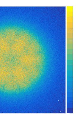
T. Braunroth et al.: EPJ Nuclear Sci. Technol. 7, 12 (2021)                              7

Table 3. Radiation lengths X0 for materials relevant to             the scattering angle θS in space is given by:
the present work.                                                                               √
          Material             X0 [g/cm ]
                                         2
                                              X0 [cm]                                    σθS = 2 σθpSx,y .                   (8)

          Uranium oxide        6.65           0.6068                In case of a compound material, the radiation length X0
          Polyethylene         44.77          50.31                 can be calculated using the formula
          Stainless steel      13.921         1.808
          Ductile iron         14.297         2.014                                       1     X wj
                                                                                             =                           (9)
          Zirconium alloy      10.223         1.558                                      X0        X0,j
                                                                                                 j

                                                                    where wj is the mass fraction of the component j and X0,j
                                                                    is the radiation length of the component j. The radiation
                                                                    lengths were either taken directly from references [34,35]
                                                                    or calculated according to equation (9). An overview of the
                                                                    various radiation lengths X0 for the relevant materials is
                                                                    given in Table 3.
                                                                       Simulations covering a broad range of kinetic energies
                                                                    were performed for all relevant materials with 105 events.
                                                                    With respect to the energy range, the same restrictions
                                                                    as for the discussion of the energy loss were applied. The
                                                                    simulated results are shown and compared to calculated
                                                                    values in Figure 6.
                                                                       The deviations between simulated and semi-empirical
                                                                    values for σθS are usually less than 3%. Only for UO2
                                                                    larger deviations of about 6% occur. In all cases, the devi-
                                                                    ations as a function of the kinetic energy remain rather
                                                                    constant. Overall, the agreement between simulated and
                                                                    calculated values is very good.

                                                                    3 Analysis and discussion
                                                                    The analysis is split into two main sections. The first sec-
                                                                    tion investigates longitudinal scans of the generic model
                                                                    and analyses simulated radiographic images. Here, the
                                                                    focus lies on the effects of various angular acceptances
                                                                    on the image quality. In addition, we compare trans-
                                                                    mission radiographic images with scattering radiographic
                                                                    images, e.g. in terms of image contrast and resolving
                                                                    power. The presentation focuses on qualitative aspects
                                                                    and is described in more detail in Section 3.1.
                                                                       The second section provides a detailed study that
                                                                    focuses on the central fuel assembly. In particular, it
                                                                    investigates the suitability of muon-scattering radiogra-
                                                                    phy to make statements about the occupancy of individual
                                                                    fuel-rod slots within a certain fuel assembly. This sec-
                                                                    tion focuses on quantitative aspects and is described in
                                                                    Section 3.2 in more detail.

Fig. 6. Comparison of root-mean square (RMS) values of scat-        3.1 Longitudinal scans covering the full cross section
tering angles (in [mrad]) between semi-empirical calculations       of the generic model
and simulated values for muons in various target materials
with a thickness of 1 mm. The top figure shows values derived       All simulations discussed in this section were performed
from the simulation (symbols) and compares them to calcu-           with 5 × 10⁷ events. All primary muons were generated at
lated values based on a semi-empirical approach (solid lines).      a fixed height (z ≈ 6.1 m) just above the generic model,
The red curve (boxes) shows the results for uranium dioxide,        while the initial x- and y-coordinates followed uniform
the orange curve (circles) corresponds to polyethylene, the blue    distributions within the limits of −1.25 m ≤ x, y ≤ 1.25 m.
curve (pentagons) corresponds to stainless steel, the green curve   This area of the initial flux is sufficient to cover the full
(up-pointing triangles) corresponds to ductile iron and the vio-    cross-section surface of the generic model.
let curve (down-pointing triangles) corresponds to zirconium          The absolute muon momenta p were treated as
alloy. The lower five figures show for each material the relative   described in Section 2.2, while different scenarios were
deviations between simulated and calculated values.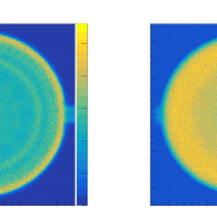
8 T. Braunroth et al.: EPJ Nuclear Sci. Technol. 7, 12 (2021)
simulated with respect to the initial muon direction. It is obvious that difference images between the two
As a first scenario (reference case), we assumed mono- geometries benefit from an improved contrast that allows
directional initial muons, i.e. p~ = −p · êz (p > 0) and identifying structural differences (or similarities) more
θin = 0◦ . In addition, we restricted the incoming muon easily. This, for instance, holds with respect to the
spectrum to various angular ranges with respect to θin . occupancy of the central fuel compartment. Even for
In particular, we considered angular distributions of 0◦ to the angular acceptance of 0◦ ≤ θin ≤ 25◦ the difference
1◦ , 0◦ to 5◦ and 0◦ to 25◦ . image provides weak evidence allowing the conclusion that
Simulations were performed for two geometries of the for both geometries the occupancies of the central fuel
generic model, which differed with respect to the occu- compartment were identical.
pancy of the fuel compartments with fuel assemblies. In
the first case, all fuel compartments were empty (no fuel
assemblies). In the second case, all fuel compartments with 3.1.2 Scattering-radiographic images
the exception of the central one were occupied with fuel Figure 8 shows scattering-radiographic images for the two
assemblies. geometries and the various angular acceptances as well
Projection images were generated using the as corresponding difference images. For each pixel, the
transmission-radiographic as well as the scattering- median of the associated scattering-angle distribution is
radiographic approach. used to generate the scattering-radiographic images.
In case of the transmission-radiographic analysis, the Similar to the transmission radiographic images, the
major imaging information is the ratio of muons reaching image quality deteriorates significantly with the increas-
the outgoing detector over the number of muons crossing ing angular acceptance with respect to θin . However, the
a specific pixel of the incoming detector. The pixel size image quality is much better and smaller structures can
was specified as (1 × 1) cm2 . be resolved. For example, the individual walls of the
In case of the scattering-radiographic analysis, the lead- fuel compartments can be easily identified for the angu-
ing imaging information is the effective scattering angle lar acceptance of 0◦ ≤ θin ≤ 1◦ and - with limitations -
θeff with respect to the initial direction, which is calculated also for the angular acceptance of 0◦ ≤ θin ≤ 5◦ . Unfortu-
event-by-event according to: nately, also the scattering-radiographic images would not
r allow for a reliable statement on the occupancy of the
2 central fuel compartment for an angular acceptance of
P di
i=x,y ∆i + ∆z · dz 0◦ ≤ θin ≤ 25◦ based on the number of simulated events.
θeff = arctan . (10) The improved resolution compared to the transmis-
zin − zout
sion radiographic images is also reflected in the differ-
ence images. With respect to the angular acceptance
of 0◦ ≤ θin ≤ 25◦ , at least the difference plot provides
The basis is given by the position information provided clear evidence that the occupancies of the central fuel
by the incoming (xin , yin , zin ) and outgoing (xout , yout , compartment are identical for both geometries.
zout ) detectors as well as the normalized muon direction
d~ = (dx , dy , dz ) provided by the incoming detector. The
projected distances ∆i (i = x, y, z) are given by iout − iin . 3.1.3 General aspects
Information on positions and directions was processed
The blurring of the structures with increasing angular
without any attempts to mimic resolution effects. Again,
acceptance can be easily understood in terms of the
the pixel size was defined as (1 × 1) cm2 .
longitudinal extension of the generic model.
In general, the simulated results show the advantages
of the scattering-radiographic over the transmission-
3.1.1 Transmission-radiographic images
radiographic approach. Here, the improved resolving
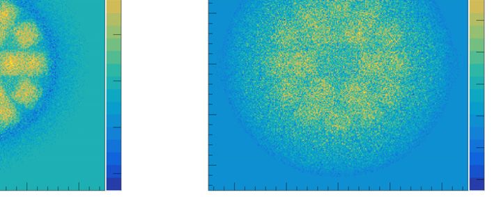
Figure 7 shows transmission radiographic images for the power is the most prominent indicator. Unlike most radio-
two geometries and the different angular distributions graphic detectors, tomographic detection systems would
with respect to θin as well as associated difference images. be able to apply cut conditions based on the incoming
It can be easily seen that the image quality in terms of muon flight directions which would allow us to realize
resolution decreases with increasing angular acceptance different angular acceptances with respect to θin .
with respect to θin . A good indicator is given in terms In summary, the simulations provide evidence that
of the absorber rods that can be easily identified for even without any reconstruction efforts to generate tomo-
the angular acceptance of 0◦ ≤ θin ≤ 1◦ . This, however, graphic images it would be possible to make conclusions
is not possible for an angular acceptance of 0◦ ≤ θin ≤ on the occupancy of specific fuel compartments with fuel
5◦ , at least not with the number of simulated events. assemblies within a reasonable amount of time. For exam-
A similar picture can be drawn for larger structures such ple, in case of an angular acceptance of 0◦ ≤ θin ≤ 25◦ and
as fuel assemblies: for the angular acceptance of 0◦ ≤ based on reasonable assumptions (see Sect. 3.2), the num-
θin ≤ 25◦ , the transmission-radiographic image based on ber of simulated events would correspond to a measuring
the simulated statistics does not allow for a reliable con- time of about 40 hours. This increases to ∼ 190 hours and
clusion on the occupancy of the central fuel compartment ∼ 930 hours in case of 0◦ ≤ θin ≤ 5◦ and 0◦ ≤ θin ≤ 1◦ ,
with a fuel assembly. respectively.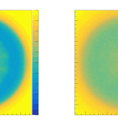
T. Braunroth et al.: EPJ Nuclear Sci. Technol. 7, 12 (2021)                                  9

Fig. 7. The figures in the two upper rows show transmission-radiographic images of longitudinal scans of a.) an empty generic
model (top row) as well as b.) a generic model filled with 18 out of 19 possible fuel assemblies (middle row) where the central fuel
compartment remained empty. The bottom row shows corresponding difference images, a − b. The color code represents the ratio of
muons that were detected in both detectors over the total number of muons. Different assumptions on the initial muon directions
are considered from left to right and range from a fixed initial muon direction with θin = 0◦ (left) to an angular distribution with
respect to θin of 0◦ to 25◦ (right). The x- and y-coordinates refer to the muon positions at the exit of the incoming detector.

   So far, these results cannot be extrapolated to smaller            All simulations were performed with up to 108 events.
structures such as individual fuel rods. Qualitatively, it         The treatment of the absolute muon momenta was iden-
can be expected that for such a level of detail a narrow           tical to the former Section 3.1. The considered angular
angular acceptance as well as a much larger muon flux per          acceptances with respect to θin of the primary muons
area would be required. The following section provides a           ranged from 0◦ ≤ θin ≤ 0.25◦ to 0◦ ≤ θin ≤ 2◦ . As in
more detailed discussion of this aspect.                           the former section, we also considered mono-directional
                                                                   incoming muons with θin = 0◦ to provide a reference sce-
                                                                   nario. The initial positions within the x, y-plane were
                                                                   restricted to −0.35 m ≤ x, y ≤ 0.35 m and the initial
3.2 Detailed longitudinal study of the central fuel                z-coordinate was fixed at z ≈ 6.1 m.
assembly to detect missing fuel rods                                  We performed simulations for two different geometries
                                                                   of the generic model. The first geometry ensured that
In this section, we investigate if muon-scattering radiog-         all fuel compartments of the model were occupied with
raphy can be used to make reliable statements about the            fuel assemblies and for each fuel assembly all individual
completeness of individual fuel assemblies. In particular,         slot positions were occupied according to the nominative
we investigate whether individual missing fuel rods in an          layout, see Figure 3. The second geometry differs from the
otherwise complete fuel assembly can be detected. This             first one only by three vacated fuel-rod positions along the
investigation takes into account a few variable boundary           diagonal (first, fifth and ninth position – see Fig. 3) within
conditions such as the angular acceptance with respect to          the central fuel assembly. The first fuel rod of interest
θin as well as the number of events, which most often can          (xid = yid = 1 (I)) is nominatively placed in the upper left
be used to provide reasonable estimates on the required            corner of the fuel assembly and is surrounded by three fuel
irradiation time.                                                  rods and the walls of the fuel compartment. The second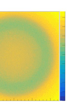
10                                      T. Braunroth et al.: EPJ Nuclear Sci. Technol. 7, 12 (2021)

Fig. 8. The figures in the two upper rows show scattering-radiographic images of longitudinal scans of a.) an empty generic
model (top row) as well as b.) a generic model filled with 18 out of 19 possible fuel assemblies (middle row) where the central fuel
compartment remained empty. The color code represents for each pixel the median of the associated scattering-angle distribution.
The bottom row shows corresponding difference images, b − a. Different assumptions on the initial muon directions are considered
from left to right and range from a fixed initial muon direction with θin = 0◦ (left) to an angular distribution with respect to θin of
0◦ to 25◦ (right). The x- and y-coordinates refer to the muon positions at the exit of the incoming detector.

                                                                     fuel rod of interest (xid = yid = 5 (II)), is surrounded by
                                                                     two control rods and six fuel rods, while the third fuel
                                                                     rod of interest (xid = yid = 9 (III)), is surrounded by fuel
                                                                     rods on all sides.
                                                                        Scattering-radiographic images were generated using a
                                                                     binning as indicated in Figure 9. Each bin covers (6.36 ×
                                                                     6.36) mm2 and is shifted in a way that for the central fuel
                                                                     assembly the center positions of the bins coincide with the
                                                                     nominative center positions within the (x, y)-plane of the
                                                                     various fuel and control rods.
                                                                        As in the previous section, the effective scattering
                                                                     angle θeff is calculated event by event according to equa-
                                                                     tion (10). For each pixel we obtain a histogram that shows
                                                                     the absolute frequencies of the effective scattering angles
                                                                     θeff . Representative examples of such absolute frequency
                                                                     distributions are shown in Figure 10.
                                                                        These frequency distributions are then normalized for
                                                                     each pixel (i, j) into a normalized probability distribution
Fig. 9. Illustration of the binning used for the analysis in Sec-    function (PDF) ρi,j (θeff ):
tion 3.2. The green disks represent the cross sections of the                           Z     π/2
various rods in the central fuel assembly. The grid indicates the                                     0          0
limits of the bins within the (x, y)-plane.                                                         dθeff ρi,j (θeff ) = 1.
                                                                                          0
T. Braunroth et al.: EPJ Nuclear Sci. Technol. 7, 12 (2021) 11
Fig. 10. Absolute frequency distributions of the effective
scattering angle θeff for different pixels and different angular Fig. 11. Probability density functions ρII (θ) (top) as well as
acceptances. The red and black curves correspond to the pixel cumulative probability functions FΘII (θ) (bottom) for the pixel
of the slot position (5,5) of the central fuel assembly. The black corresponding to the slot position with xid = yid = 5 within
curve represents the case where this particular slot position is the central fuel assembly for two different geometries. The red
empty while the red curve corresponds to the case where the slot curve represents the geometry with a complete fuel assembly
position is filled with a fuel rod. The blue curve corresponds to (all positions are occupied according to the nominative layout),
a pixel between two neighbouring fuel assemblies. The top fig- while the black curve corresponds to the geometry where the
ure shows results for a fixed angular acceptance (θin = 0◦ ) while specific slot position represented by this pixel is empty. The
the bottom figure shows results for an angular acceptance of distributions represent results of a simulation with 108 events
0◦ ≤ θin ≤ 2◦ . All distributions correspond to simulations with assuming mono-directional muons with θin = 0◦ .
108 events.
We consider for each pixel (i, j) in the (x, y)-plane the
two-sample Kolmogorov-Smirnov test,
In a final step, we use ρi,j (θeff ) to calculate for each pixel
i, j the cumulative distribution function (CDF) FΘi,j (θeff ), Di,j = sup |FΘocc
i,j
(θeff ) − FΘvac
i,j
(θeff ) |, (11)
i.e.: θeff
Z θ which allows us to make quantitative statements on the
0 0
FΘi,j (θeff ) = dθeff ρi,j (θeff ). agreement between FΘocc i,j
(θeff ) and FΘvac i,j
(θeff ).
0
The null hypothesis - i.e. FΘocc i,j
(θ eff ) and FΘvac
i,j
(θeff )
This procedure is repeated for each simulation. describe identical distributions – is rejected at a statistical
For illustration, Figure 11 shows for both geometries the significance level α if the test statistic satisfies
PDF ρII as well as the CDF FΘII corresponding to the s
pixel of the slot position with xid = yid = 5 within the cen- i,j ni,j + mi,j
D > c(α)
tral fuel assembly. The analysis focuses on a pixel-based ni,j · mi,j
comparison between the two geometries described above. p
By computing the local distances between the empirical c(α) = −0.5 · ln (α/2).
CDFs, the derived statistical measure can be used for the
pair-wise comparison of images [38,39]. In other words, Here ni,j (mi,j ) describes the number of entries in the
we compare for each pixel i, j the CDFs FΘocc (θeff ) and (i, j) pixel of the relevant vacated (occupied) spectrum.
i,j
The condition can be reformulated as:
FΘvac
i,j
(θ eff ). Here, F occ
Θi,j (θ eff ) corresponds to the geometry
for which all slot positions within the fuel assemblies are Di,j ni,j · mi,j
r
occupied, while FΘvac (θeff ) corresponds to the geometry D̃i,j ≡ > 1. (12)
i,j c(α) ni,j + mi,j
for which the fuel-rod slot positions within the central
fuel assembly are empty. We specified the significance level α of 0.1 in the following.12 T. Braunroth et al.: EPJ Nuclear Sci. Technol. 7, 12 (2021)
Fig. 12. A heat map showing the significance ratio D̃ in
the (x, y)-plane. One can easily identify the locations of the
three vacated fuel-rod slot positions along the diagonal. The
spectrum represents simulations with 108 events assuming
mono-directional muons.
Fig. 13. Significance ratios D̃i,j as a function of angular accep-
Figure 12 shows a heatmap of D̃i,j based on a simu-
tance with respect to θin and simulated events for the three pixels
lation with 108 events assuming mono-directional muons
of interest. The top figure shows the results of DI , while DII
with θin = 0◦ . One can clearly identify areas for which (DIII ) is shown in the middle (bottom) figure.
the Kolmogorov-Smirnov test statistic indicates signifi-
cant deviations. These areas coincide perfectly with areas
for which the two geometries differ, i.e. with respect to (4 · 107 events) are required for D̃II to exceed one for
the occupation of the slot positions xid = yid = 1 (I), 0◦ ≤ θin ≤ 0.5◦ , we also observe significant deviations with
xid = yid = 5 (II) and xid = yid = 9 (III) within the respect to 0◦ ≤ θin ≤ 0.75◦ . For the latter, at least 5 · 107
central fuel assembly. simulations events are required for D̃II to exceed one. In
Figure 13 summarizes D̃i,j for each of these three par- case of pixel III, we observe that D̃III also exceeds one
ticular pixels and for different angular acceptances and for 0◦ ≤ θin ≤ 1.0◦ , requiring at least 8.5 · 107 simulated
quantifies the evolution as a function of simulated events. events. The significant deviations between the individual
D̃I corresponds to the pixel of xid = yid = 1, while D̃II pixels may be related to the larger numbers of neighbour-
and D̃III correspond to the pixels of xid = yid = 5 and ing fuel rods in case of pixels II and III compared to
xid = yid = 9, respectively. pixel I.
It is obvious that for all three pixels the significance For a specific simulation with known momentum dis-
ratios D̃ decrease in general with an increasing angular tribution and angular acceptance, the measurement time
acceptance. The only exception is given in terms of the can be estimated according to the following formula:
angular acceptances 0◦ ≤ θin ≤ 1.5◦ and 0◦ ≤ θin ≤ 2◦ ,
simulated events
for which comparable significance ratios are observed. For ∆t[s] = . (13)
all three pixels one can observe a clear trend towards A[cm2 ] · Iµ [muons/cm2 /s] · Iθin · Ip ·
smaller slopes of progression with an increasing angular
acceptance and increasing number of simulated events. Here, A is the area of the initial (x, y)-plane, Iµ is the inte-
It is interesting to note that there are significant differ- grated muon flux at sea level (∼ 1 muon/cm2 /min), Iθin is
ences between the three pixels with respect to the trends the share within the angular acceptance with respect to
with increasing event numbers and the achieved signifi- θin , Ip is the share of the considered momentum distribu-
cance ratios. These effects are stronger for pixel II (III) tion with respect to the full momentum distribution and
compared to I. With respect to pixel I and based on is the efficiency of the detector system, which is assumed
the maximum number of events (108 ), the significance to be 1 in the following. For a certain angular acceptance,
Iθin can be estimated according to:
ratio D̃I exceeds one only up to an angular acceptance
of 0◦ ≤ θin ≤ 0.5◦ and requires at least 6 · 107 simulated R θin 0
events in case of the latter. A different picture can be 0
dθ cos2 θ0
Iθin = R π/2 . (14)
drawn for pixel II. Not only do we observe that less events 0
dθ0 cos2 θ0T. Braunroth et al.: EPJ Nuclear Sci. Technol. 7, 12 (2021) 13
Table 4. Estimations for Iθin for various angular accep- into smaller measurement times; on the contrary, larger
tances. angular acceptances lead to extended measurement times.
[0◦ ; 0.5◦ ] [0◦ ; 1◦ ] [0◦ ; 2◦ ] [0◦ ; 5◦ ] [0◦ ; 25◦ ]
Iθin [%] 1.11 2.22 4.44 11.08 52.16 4 Summary and conclusion
In this work we investigated the theoretical feasibility to
detect individual missing fuel rods in an otherwise fully
loaded cask within a reasonable amount of time using
cosmic muons. We used simulations based on the Geant4
toolkit and a generic model based on the CASTOR R V/19
(see Fig. 2) loaded with 18x18-24 PWR fuel assemblies
(see Fig. 3). The detectors above and below a verti-
cal (standing) model were mimicked by two rectangular
planes with vanishing thickness and an area of 9 m2 .
The gap between detectors and the model was assumed
to be 10 cm. The muon characteristics are described
in Section 2.2. The tool can be run with a realistic
muon spectrum but also allows for performing simu-
lations assuming mono-energetic and mono-directional
muons. For validation purposes, the stopping powers
(see Fig. 5) and scattering angles (see Fig. 6) of the
relevant target materials have been investigated and
compared against established reference values from the
literature. We found good agreement between simulated
and literature/analytical values.
We simulated longitudinal scans that covered the full
cross section of the model (full-model simulation). In addi-
tion, we put a special emphasis on a single fuel assembly
with missing fuel rods.
The focus of the full-model simulation was on the
effect of angular acceptance criteria on the resolution.
We compared mono-directional muons (θin = 0◦ ) with
different angular acceptance ranges with respect to θin :
Fig. 14. Significance ratios D̃i,j for different angular accep- 0◦ ≤ θin ≤ 1◦ , 0◦ ≤ θin ≤ 5◦ and 0◦ ≤ θin ≤ 25◦ . The inte-
tances with respect to θin as a function of the estimated
grated flux was kept constant with 5·107 muons, which
measurement time for the three pixels of interest. The top figure
corresponds to a radiation time of approximately 40 hours
shows the results of DI , while DII (DIII ) is shown in the middle
(bottom) figure.
in case of 0◦ ≤ θin ≤ 25◦ . We performed two analyses and
compared the empty model with a partially loaded one
and the resulting difference between the two radiographic
Values of Iθin for various angular acceptances are listed images. The partially loaded model was lacking the central
in Table 4. In a similar way, a simplified estimate of Ip fuel assembly. In the first analysis (transmission radio-
(≈ 0.8) can be determined by means of equation (1): graphic scans) we compared the ratio of muons in the
lower and upper detectors. This radiographic analysis
R p(T =1 TeV)
dp0 I(p0µ , 0) clearly indicated the decreasing resolution with increas-
p(T =1 GeV)
Ip = R∞ . (15) ing angular acceptance with respect to θin of the incoming
0
dp0 I(p0µ , 0) muons (see Fig. 7). The central fuel assembly could still
be identified as missing based on the difference plot of
Figure 14 summarizes D̃i,j for each of the three pixels of the acceptance criteria 0◦ ≤ θin ≤ 25◦ . In addition, we
interest and quantifies the evolution as a function of the repeated the analysis with a focus on the effective scatter-
estimated measurement time. ing angles of the muons to receive scattering-radiographic
In case of an angular acceptance of 0◦ ≤ θin ≤ 0.5◦ , images. The image quality was much better compared to
at least ∼ 1.8 years are required for a reliable statement the transmission-radiographic analysis and more details
for pixel II. Longer measurement times are required for could be identified (see Fig. 8). Again, for the acceptance
pixels I (∼ 2.6 years) and III (∼ 2.2 years). Smaller criteria of 0◦ ≤ θin ≤ 25◦ the difference plot can be used
measurement times are expected for the smaller angu- to identify the central fuel assembly as missing.
lar acceptance of 0◦ ≤ θin ≤ 0.25◦ : Here, the estimated We further investigated the capability of muon-
measurement times amount to ∼1.8 years (I and II) scattering radiography to provide reliable statements on
and ∼0.9 years (III), respectively. Overall and based on the completeness of a loaded fuel assembly, assuming up
the assumptions of the present work, the statistical ben- to 108 events and angular acceptance criteria of 0◦ ≤ θin ≤
efit of a larger angular acceptance does not translate 0.25◦ , 0◦ ≤ θin ≤ 0.5◦ , 0◦ ≤ θin ≤ 0.75◦ , 0◦ ≤ θin ≤ 1.0◦ ,14 T. Braunroth et al.: EPJ Nuclear Sci. Technol. 7, 12 (2021)
0◦ ≤ θin ≤ 1.5◦ and 0◦ ≤ θin ≤ 2.0◦ in addition to mono- arbitrarily selected three fuel rods and it may be worth
directional muons with θin = 0◦ . Focussing on the central the effort to repeat the analyses systematically, including
fuel assembly we investigated a fully loaded model and the effects of rods in the immediate surroundings. The sig-
one where the central assembly was missing three fuel nificance information of the second analysis part is derived
rods on the diagonal (see Fig. 3). All three missing from two predominantly identical geometries, which devi-
rods were clearly identifiable after the simulation of 108 ated only by the occupation of three fuel rod slots. It
events assuming mono-directional muons with θin = 0◦ would be insightful to investigate the effects of additional
(see Fig. 12). The significance ratio D̃ based on the differences such as slight misalignments. In addition, we
Kolmogorov-Smirnov test statistic of each fuel rod (and intend to investigate the sensitivity of the simulation
thus the significance of the contrast of a missing rod) results to the physics models in Geant4. The present work
depends on the relative position of the missing fuel rod in focuses on the modular physics list FTFP BERT.
the assembly, the angular acceptance criteria of incoming The fourth aspect addresses the extension to tomo-
muons and the number of simulated events (see Fig. 13). graphic images which allows using the complete infor-
The latter can be transformed accordingly into radiation mation of scattered (or absorbed) muons within one
or measuring times. Assuming significance ratios D̃i,j > 1 visualization processed by various potential statistical
leading to a successful identification of missing fuel rods muon-tomography reconstruction algorithms as discussed
we found measuring times of approximately 2 years for in [40]. For adaptively comparing muon-scattering (or
the two inner missing rods and ∼2.6 years for the corner absorption) images of a cask with the purpose of automat-
rod assuming an angular acceptance of 0◦ ≤ θin ≤ 0.5◦ . ically detecting changes within the interior of the cask, the
In summary, we have shown that the muon-scattering image-processing strategy needs to be extended towards
radiography is capable of reliably visualizing the inside of tomographic image reconstruction inherently designed for
a loaded and sealed model at a resolution scale of a sin- change detection or in combination with further image
gle fuel rod. The assumptions we made led to timescales analysis methods.
which seem feasible compared to the duration of the dry We intend to make the developed simulation code avail-
storage of spent nuclear fuel. In the next section we discuss able in the near future. If interested, please contact the
how future work might even shorten the theoretically esti- main author for more details.
mated measuring time and how image processing methods
may be used to gain more detailed insights into the cask’s This research was partially funded by the Federal Ministry for
interior for the detection of individual missing fuel rods. the Environment, Nature Conservation and Nuclear Safety in
Germany (BMU) under Contract 4720E03366.
5 Outlook
Author contribution statement
The present work will serve as a starting point for
further research activities that may evolve into several All the authors were involved in the preparation of the
independent aspects. manuscript. All the authors have read and approved the
The first aspect relates to the developed simulation tool final manuscript.
itself. We intend to include the discussion of transversal
scans, for which the detectors are located on the sides of
the generic model. The simulation can also be extended References
to additional geometries which do not have to be limited
to storage casks. 1. K.-P. Ziock, G. Caffrey, A. Lebrun, L. Forman, P. Vanier,
The second aspect treats the validation of the sim- J. Wharton, IEEE Nuclear Science Symposium Conference
ulated data and comparisons to other simulations. We Record, 2005, Fajardo, 2005, pp. 1163–1167
already addressed validation aspects in the present work 2. V. Brdar, P. Huber, J. Kopp, Phys. Rev. Appl. 8, 2331
that concerned the slowing-down process of the muons as (2017)
well as the angular scattering. A logical next step would 3. G. Bonomi, P. Checchia, M. D’Errico, D. Pagano, G.
be given by a comparison of simulated to experimental Saracino, Prog. Part. Nucl. Phys. 112, 103768 (2020)
4. P.A. Zyla et al. (Particle Data Group), Prog. Theor. Exp.
results. For this it might be reasonable to start with less
Phys. 2020, 083C01 (2020)
complex geometries or larger objects-of-interest which will 5. M.P. De Pascale et al., J. Geophys. Res. A 98, 3501 (1993)
require less time, both with respect to the computation 6. P.K.F. Grieder, Cosmic Rays at Earth (Elsevier Science,
and the experimental measurement. To take into account Amsterdam, 2001)
the uncertainty due to a particular choice of the simu- 7. L.W. Alvarez et al., Science 167, 832–839 (1970)
lation tool, it would be valuable to compare the results 8. H.K.M. Tanaka, T. Kusagaya, H. Shinohara, Nat. Commun.
from different simulation tools for identical geometries for 5, 3381 (2014)
benchmark purposes. 9. N. Lesparre, D. Gilbert, J. Marteau, Y. Déclais, D. Carbone,
The third aspect covers to sensitivity analyses. The E. Galichet, Geophys. J. Int. 183, 1348–1361 (2010)
present results indicate that the significance depends on 10. K. Morishima et al., Nature 552, 386–390 (2017)
the relative fuel rod position and, hence, the immedi- 11. H.K.M. Tanaka, K. Nagamine, S.N. Nakamura, K. Ishida,
ate surroundings of the considered rod. So far, we have Nucl. Instrum. Methods Phys. Res. A 555, 164–172 (2005)You can also read