Voluntary and Mandatory Social Distancing: Evidence on COVID-19 Exposure Rates from Chinese Provinces and Selected Countries 8243 2020 - ifo ...
←
→
Page content transcription
If your browser does not render page correctly, please read the page content below
8243
                                                          2020
                                                           April 2020

Voluntary and Mandatory
Social Distancing: Evidence on
COVID-19 Exposure Rates from
Chinese Provinces and
Selected Countries
Alexander Chudik, M. Hashem Pesaran, Alessandro Rebucci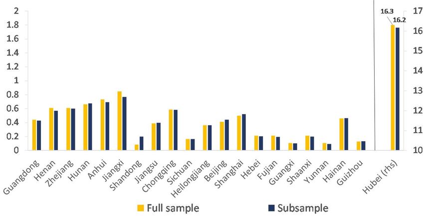
Impressum:

CESifo Working Papers
ISSN 2364-1428 (electronic version)
Publisher and distributor: Munich Society for the Promotion of Economic Research - CESifo
GmbH
The international platform of Ludwigs-Maximilians University’s Center for Economic Studies
and the ifo Institute
Poschingerstr. 5, 81679 Munich, Germany
Telephone +49 (0)89 2180-2740, Telefax +49 (0)89 2180-17845, email office@cesifo.de
Editor: Clemens Fuest
https://www.cesifo.org/en/wp
An electronic version of the paper may be downloaded
· from the SSRN website:       www.SSRN.com
· from the RePEc website:      www.RePEc.org
· from the CESifo website:     https://www.cesifo.org/en/wp

CESifo Working Paper No. 8243

       Voluntary and Mandatory Social Distancing:
       Evidence on COVID-19 Exposure Rates from
        Chinese Provinces and Selected Countries
                                                Abstract

This paper considers a modification of the standard Susceptible-Infected-Recovered (SIR)
model of epidemic that allows for different degrees of compulsory as well as voluntary social
distancing. It is shown that the fraction of population that self-isolates varies with the perceived
probability of contracting the disease. Implications of social distancing both on the epidemic and
recession curves are investigated and their trade-off is simulated under a number of different
social distancing and economic participation scenarios. We show that mandating social
distancing is very effective at flattening the epidemic curve, but is costly in terms of
employment loss. However, if targeted towards individuals most likely to spread the infection,
the employment loss can be somewhat reduced. We also show that voluntary self-isolation
driven by individual’s perceived risk of becoming infected kicks in only towards the peak of the
epidemic and has little or no impact on flattening the epidemic curve. Using available statistics
and correcting for measurement errors, we estimate the rate of exposure to COVID-19 for 21
Chinese provinces and a selected number of countries. The exposure rates are generally small,
but vary considerably between Hubei and other Chinese provinces as well as across countries.
Strikingly, the exposure rate in Hubei province is around 40 times larger than the rates for other
Chinese provinces, with the exposure rates for some European countries being 3-5 times larger
than Hubei (the epicenter of the epidemic). The paper also provides country-specific estimates
of the recovery rate, showing it to be about 21 days (a week longer than the 14 days typically
assumed), and relatively homogeneous across Chinese provinces and for a selected number of
countries.
JEL-Codes: D000, F600, C400, I120, E700.
Keywords: COVID-19, SIR model, epidemics, exposed population, measurement error, social
distancing, self-isolation, employment loss.

              Alexander Chudik                                        M. Hashem Pesaran
     Federal Reserve Bank of Dallas / USA                    University of Southern California / USA
        alexander.chudik@dal.frb.org                                    pesaran@usc.edu
                                        Alessandro Rebucci
                           Johns Hopkins University Carey Business School
                                         arebucci@jhu.edu
April 15, 2020
We thank Johns Hopkins University for assistance with the data. We would also like to acknowledge helpful
comments by Ron Smith. The views expressed in this paper are those of the authors and do not necessarily reflect
those of the Federal Reserve Bank of Dallas.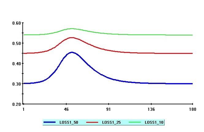
1    Introduction

The COVID-19 pandemic has already claimed many lives and is causing an unprecedented and

widespread disruption to the world economy. China responded to the initial outbreak with dra-

conian social distancing policies which are shown to be e¤ective in containing the epidemic, but at

the cost of large short term losses in employment and output. Other countries have responded more

timidly, either by deliberate choice, as in the United States, or due to implementation constraints,

as in some European countries. The purpose of this paper is to evaluate the impact of alternative

mitigation or containment policies on both the epidemic and the so-called recession curves, and to

empirically compare their implementation across countries.

    Most importantly we consider both government-mandated social distancing policies, and vol-

untary self-isolation, and endogenize the fraction of the population that remain exposed to the

virus within a standard Susceptible-Infected-Recovered model (SIR). Speci…cally, we distinguish

between individuals exposed to COVID-19 and those isolated from the epidemic. We decompose

the population, P , into two categories: those who are exposed to COVID-19 in the sense that they

can contract the virus because they are not isolated and they have not been infected yet, PE ; and

the rest, PI , that are isolated and therefore taken out of harm’s way. We denote the strength of the

mitigation policy by 1     , where   is the proportion of population that is exposed to COVID-19,

de…ned as    = PE =P . Initially we focus on the relatively simple case where    is set at the outset

of the spread of the epidemic, close to what we believe China did after the start of the epidemic

in Wuhan. We also consider a variation of the SIR model where         changes due to the voluntary

decision to isolate at the micro level. Using a simple decision model we show that the proportion of

the population that self-isolates rises with the probability of contracting the disease. We approxi-

mate this probability with the number of active cases and show (by simulation) that the e¤ect of

self-isolation occurs as the epidemic nears its peak, and is relatively unimportant during the early

or late stages of the epidemic. A coordinated social policy is required from the early outset of the

epidemic to ‡atten the epidemic curve.

    We then model the short-term impact of the epidemic on employment. This permits an eval-

                                                 1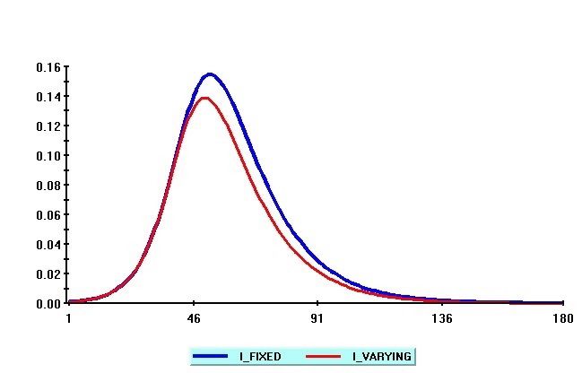
uation of the costs and bene…ts of alternative societal decisions on the degree and the nature of

government-mandated containment policies by considering alternative values of            in conjunction

with an employment loss elasticity, , that allows a given social distancing policy to have di¤erent

employment consequences. In the extreme case where the incidence of social distancing is uniform

across all individuals and sectors, a fall in     results in a proportionate fall in employment, and

  = 1. But by enabling individuals to isolate and to work from home, together with wide spread

targeted testing for the virus plus the use of protective clothing and equipment, it is possible to

mitigate somewhat the economic costs of social distancing policies. We simulate the employment

loss for alternative values of   and    and …nd that, for su¢ ciently low values of    required to man-

age the peak of hospitalization and death from COIVD-19, the economic costs could be substantial

even with smart social distancing policies. We also simulate the duration of the epidemic to be

around 120 days, with a sizeable part of the employment loss occurring close to the peak of the

epidemic.

      Whilst there is ample medical and biological evidence on the key parameters of the SIR model,

namely the basic reproduction rate, R0 , and the recovery rate, , to our knowledge there are no

direct estimates of . A recent report from the Imperial College COIVD-19 Response Team uses

a Bayesian hierarchical model to infer the impact of social distancing policies implemented across

11 European countries, see Flaxman et al. (2020). They use the number of observed deaths to

infer the number of infections and do not make use of con…rmed infections that are subject to

signi…cant measurement errors due to limited testing. Whilst acknowledging the measurement

problems, in this paper we provide estimates of         and   using daily data on con…rmed, recovered

and death cases from the Johns Hopkins University (JHU) hub.1 Using a discretized version of our

modi…ed SIR model we derive reduced form regressions in con…rmed recoveries and the number of

active cases that allow for systematic and random measurement errors. We show that              can be

identi…ed assuming that con…rmed infected and recovery cases are subject to a similar degree of

mis-measurement. We also show that, for a given value of R0 , the social distancing parameter, ;

can be identi…ed up to a fraction which is determined by the scale of mis-measurement of reported
  1
      Available at https://github.com/CSSEGISandData/COVID-19/tree/master/csse_covid_19_data.

                                                    2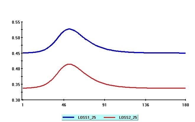
active cases. We calibrate this fraction using the data from the Diamond Princess cruise ship

reported by Moriarty et al. (2020).

   We …rst use daily data on Chinese provinces with complete history of the course of the epidemic.

The estimates of the recovery rates are very similar across the Chinese provinces and lie in the range

of 0.033 (for Beijing) and 0.066 (for Hebei). We also …nd that the random measurement in the

underlying data is relatively unimportant for the estimation of . The mean estimate of     across the

Chinese provinces is around 0:046 which corresponds to around 22 days from infection to recovery

(or death). This estimate is substantially larger than the 14 days typically assumed in designing

quarantine policies. Setting    = 0:046 and R0 , we then proceed to estimate       (up to the scaling

fraction). We …nd that for Chinese provinces    is very small even if we allow for a signi…cant under-

recording of infected and recovered cases. We …nd that, with the exception of Hubei province (the

epicenter of the epidemic), the share of exposed population across other provinces was less than 1

individuals per 100,000! This is an astonishingly low rate and is consistent with dramatically falling

estimates of the e¤ective reproduction rate at the onset of the epidemic in China. In contrast, the

estimates of   which we have obtained for European countries are signi…cantly higher even when

compared to the relatively high exposure rates for Hubei, with a substantial heterogeneity across

countries. In particular, we estimate exposure rates for Italy and Spain to be almost …ve times the

rate estimated for Hubei.

   To summarize, our theoretical analysis shows that voluntary social distancing is likely to be ef-

fective only when the epidemic begins to approach its peak, and mandated social distancing to ‡atten

the curve is required from the early phases of the epidemic. Our estimates show that in order to

‡atten the epidemic curve very strict mandatory policies are necessary, as in the case of the Chinese

provinces excluding the Hubei epicenter show. Unfortunately, our estimates suggest that, despite

the time-lag in the contagion from China to other countries, an inadequate and uncoordinated policy

response resulted in exposure rates outside of China that are multiples of those documented at the

epicenter of the epidemic in Hubei.

Related Literature

   The characteristics and the economic consequences of the COVID-19 outbreak, and of policies

                                                  3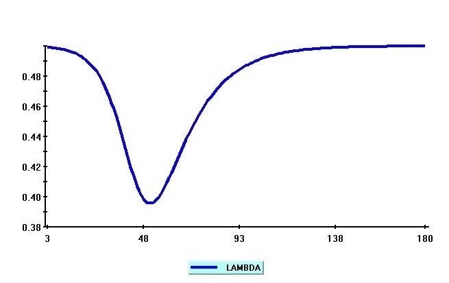
to contain its spread, are the subject of a fast growing body of research. Scienti…c evidence based

on more accurate data at the local level has begun to document the rate of transmission and

incubation periods. The literature has also begun to document the role of mitigation policies in

reducing transmission, and the rate of asymptomatic transmission.

   Kucharski et al. (2020) estimate that, in China, the e¤ective reproductive rate Rt fell from

2.35 one week before travel restrictions were imposed on Jan 23, 2020, to 1.05 one week after travel

restrictions. They use a SIR model and estimate it to forecast the epidemic in China, extending

the model to explicitly account for infections arriving and departing via ‡ights. Using data from

Wuhan, Wang et al. (2020) report a baseline reproductive rate of 3.86, that fell to 0.32 after the

vast lock-down intervention. They also …nd a high rate of asymptomatic transmission.

   Work on the economic impact of the epidemic is just starting, as the data are only partially

available. Atkeson (2020) explores the trade-o¤ between the severity and timing of suppression

of the disease, for example through social distancing, and the progression of the disease in the

population in simulations of a SIR model like ours with exposed and not exposed population, but

does not provide estimates and does not focus on the share of the exposed population, nor does he

provides estimates of the model parameters.

   Berger, Herkenho¤, and Mongey (2020) show that testing at a higher rate in conjunction with

targeted quarantine policies can reduce both the economic impact of the COIVD-19 and peak

symptomatic infections. As noted above, by selectively applying social distancing policies (with

di¤erent   parameters) it is also possible to reduce both the economic impact of the epidemic and

the peak symptomatic infections. Related to this, using data on the Spanish ‡ue, Correia, Luck,

and Verner (2020) …nd that cities that intervened earlier and more aggressively do not perform

worse and, if anything, grow faster after the pandemic is over. These …ndings thus indicate that

containment policies not only lower mortality, they also mitigate the adverse long term economic

consequences of a pandemic.

   Fang, Wang, and Yang (2020) analysis of Chinese e¤orts to contain the COIVD-19 outbreak

measures the e¤ectiveness of the lock-down of Wuhan and enhanced social distancing policies in

other cities. They produce evidence for all Chinese provinces and show that these policies con-

                                                 4
tributed signi…cantly to reducing the total number of infections outside of Wuhan.
Stock (2020) focuses on measurement error and explores the bene…ts of randomly testing the
general population to determine the asymptomatic infection rate.
Eichenbaum, Rebelo, and Trabandt (2020) discuss the trade o¤ between the economic costs of
containment policies — which could include a recession — and the number of lives saved in a model
in which agents optimize and the probability of infection is endogenous. Barro, Ursua, and Weng
(2020) estimate death rates and output losses based on 43 countries during the 1918-1920 Spanish
‡u. They …nd a very high death rate, with 39 million deaths, or 2.0 percent of world population,
implying 150 million deaths when applied to current population. According to their estimates, the
Spanish ‡ue resulted in economic declines for GDP and consumption in the typical country of 6
and 8 percent, respectively.
Linton (2020) uses a reduced form quadratic time trend model in log of new cases and new
deaths to predict the peak of COIVD-19 for a large number of countries.
As far as we are aware, no study has modelled the di¤erence between government-mandated
and self-imposed isolation and their implication for the ‡attening of the economic and pandemic
curves that we consider in this paper.
The rest of the paper is organized as follows. Section 2 sets out the modi…ed SIR model with
social distancing. Section 3 analyzes the distinction between mandatory and voluntary isolation.
Section 4 discusses the trade o¤ between containing the epidemic and the employment losses that
depend on the share of exposed population. Section 5 sets out the econometric and measurement
models and reports the estimation results. Section 6 concludes.
2 A Discrete-time SIR Model with Mitigation Policy
There are many approaches to modelling the spread of epidemics. The basic mathematical model
used by many researchers is the susceptible-infective-removed (SIR) model advanced by Kermack
and McKendrick (1927). This model, and its various extensions, has been the subject of a vast
number of studies, and has been used extensively over the past few months to investigate the spread
5of COVID-19. A comprehensive treatment is provided by Diekmann and Heesterbeek (2000) with
further contributions by Metz (1978), Satsuma et al. (2004), Harko et al. (2014), Salje et al.
(2016), amongst many others.
The basic SIR model considers a given population of …xed size P , composed of three distinct
groups, those individuals in period t who have not yet contracted the disease and are therefore
susceptible, denoted by St ; the ‘removed’ individuals who can no longer contract the disease,
consisting of recovered and deceased, denoted by Rt ; and those who remain infected at time t and
denoted by It . Thus
P = St + It + Rt : (1)
As it stands, this is an accounting identity, and it is therefore su¢ cient to model St and It and
obtain Rt as the remainder. The SIR model is typically cast in a set of di¤erential equations, which
we discretize and write as the following di¤erence equations (for t = 1; 2; :::; T )
St+1 St = st It ; (2)
It+1 It = ( st )It ; (3)
Rt+1 Rt = It ; (4)
where and are the key parameters of the epidemic. is the rate of transmission and is
the recovery rate. In this model it is assumed that an infected individual in period t causes st
secondary infections, where st = St =P is the share of susceptible individuals in the total population.
The time pro…le of It critically depends on the basic reproduction number, de…ned as the expected
number of secondary cases produced by a single infected individual in a completely susceptible
population, denoted by R0 = = . The parameter is determined by the biology of the virus, and
is assumed to be constant over time and homogeneous across countries and regions. The recovery
rate, , can also be written as = 1=d, where d denotes the number of days to recover or die
from the infection. We assume that is constant over time, but allow it to vary across countries
and regions, re‡ecting the di¤erences in the capacity of the local health care systems to treat the
infected population.
6The epidemic begins with non-zero initial values I1 > 0 and S1 > 0, and without any mitigation
policies in place it will spread widely if R0 > 1, ending up infecting a large fraction of the population
if R0 is appreciably above unity. We show below that the steady state value of this proportion is
given by 0 = (R0 1)=R0 . In the case of COVID-19, a number of di¤erent estimates have been
suggested in the literature, placing R0 somewhere in the range of 2:4 to 3:9.2
In the simulations, and the empirical analysis to follow, we adopt a central estimate and set
R0 = 3. As we shall see the SIR model predicts that in the absence of social distancing as much
as 2/3 of the population could eventually become infected before the epidemic runs its course–
the so-called herd immunity solution to the epidemic. Such an outcome will involve unbearable
strain on national health care systems and a signi…cant loss of life, and has initiated unparalleled
mitigation policies …rst by China and South Korea, and more recently by Europe, US and many
other countries. Such interventions, which broadly speaking we refer to as "social distancing",
include case isolation, banning of mass gatherings, closures of schools and universities, and even
local and national lock-downs.
To investigate the economic implications of such policies we …rst modify the SIR model by
decomposing the total population, P into two categories, those who are exposed to COVID-19 in
the sense that they could catch the virus (they have not been infected yet), PE , and the rest, PI ,
who are isolated and therefore taken out of harm’s way. We denote the strength of the mitigation
policy by 1 ; where is the proportion of population that is exposed to COVID-19, de…ned as
= PE =P . In practice, will be time-varying and most likely there will be feedbacks from the
progress of the epidemic to the coverage of the intervention policies. Here we consider the relatively
simple case where is set at the outset of the spread of the epidemics, close to what we believe
China did after the start of the epidemic in Wuhan.
In the presence of the social distancing intervention characterized by , the equations of the
2
Using data from Wuhan, Wang et al. (2020) report a pre-intervention reproductive rate of 3.86. Kucharski et al.
(2020) estimate that, in China, the reproductive rate was 2.35 one week before travel restrictions were imposed on
Jan 23, 2020. Ferguson et al. (2020) made baseline assumption of R0 = 2:4 based on the …ts to early growth-rate of
epidemic in Wuhan (and also examined values of 2.0 and 2.6) based on …ts to the early growth-rate of the epidemic
in Wuhan by Li et al. (2020) and Riou and Althaus (2020).
7SIR model now become (noting that the population exposed to the virus is now PE ):
St
St+1 St = It ;
PE
St
It+1 It = It ,
PE
P = St + It + Rt :
Dividing both sides of the above equation by P and using the fractions st = St =P , it = It =P and
rt = Rt =P , we have
st+1 st = st it ; (5)
it+1 it = st it , (6)
and
= st + it + rt . (7)
Given , the fraction of total exposed population, , determines the e¤ective transmission rate,
= = . When = 1, the whole population is exposed, and the e¤ective transmission rate
coincides with the biological one, .
The system equations (5) and (6) can be solved by iterating forward from some non-zero initial
values, with i1 a small fraction and s1 = i1 , since at the start of the epidemic we can safely
assume that r1 = 0. Iterating (6) forward from i1 > 0, and for given values of s1 ; s2 ; :::st we have
(where we have replaced = = = (R0 = ))
t
!
Y
it+1 = i1 ; (8)
=1
where = 1+ [(R0 = ) s 1]. Initially, where few are infected and s is close to , > 1 and the
number of infected individuals rises exponentially fast so long as R0 > 1. But as the disease spreads
and recovered and/or deceased are removed, at some point in time t = t , s starts to fall for > t
Qt
such that < 1 from > t ; and eventually limt!1 =1 = 0. Hence, limt!1 (it ) = i = 0.
8Further, limt!1 (it+1 =it ) = 1, and from (6) we have limt!1 st = s = ( = ) = =R0 , and using
the identity = s + r , we …nally obtain the following expression for the total number of infected
cases as a fraction of the population (c ):
(R0 1)
c =r = =R0 = : (9)
R0
The choice of also has important implications for the steepness and and the peak of the
epidemic curve, and can be used to ‡atten the trajectory of it . To this end, and also for the
purpose of estimating using data realizations from completed epidemics, we …rst eliminate st
from the equation for it noting from (6) and (5) that
st+1 it+1
=1 it and =1 + st . (10)
st it
it+1
Since > 0, solving for st , we have st = it 1+ , and hence
it+2
st+1 it+1 1+
= =1 it ;
st it+1
1+
it
which yields the following second-order non-linear di¤erence equation in it
it+1 = i2t =it 1 + it it 1 (1 ) i2t ; t = 1; 2; :::; T; (11)
with the initial values i1 and i2 = (1 + s1 ) i1 , where s1 = i1 . Realizations on it , for
t = 1; 2; :::; T , can also be used to estimate and from the above non-linear autoregression,
but it is important to note that and cannot be separately identi…ed without further a priori
knowledge. In the empirical analysis that follows we set R0 a priori and estimate from R0 = , as
= R0 and = = .
As an illustration in Figure 1 we show the time pro…le of it ( ) using the parameter values R0 = 3
and = 1=d = 1=14 and the initial values i1 ( ) = =1000; and i2 ( ) = [1 + ( R0 = ) s1 ( )] i1 ( ),
where s1 ( ) = i1 . Consider the following social distancing coe¢ cients, = 1; 0:75, and 0:50.
9The time pro…les of the infected (as the fraction of population) peak after 52 days and does not
seem to depend much on the choice of . But the choice of is clearly important for ‡attening the
curve and reduces the peak of infected from 31 percent when = 1, to 23 per cent for = 0:75;
and to 15 per cent for = 0:50.
Figure 1: Simulated values of it ( ) for di¤erent social distancing coe¢ cients: = 1 (blue); 0:75
(red), and 0:5 (green)
3 A voluntary model of social isolation: case of time-varying
So far we have assumed that , the proportion of population that can be infected is …xed and
set exogenously by central authorities. In practice, the degree of social distancing also depends
on the extent to which individuals follow the rules, which could depend on the fear of contracting
the disease and most likely will depend on the number of those who are already infected, and
an individual’s perception of the severity of the epidemic and its rate of spread. Even central
authorities can be slow to respond when the number of active cases is small and they might delay
or start with a low level of social distancing and then begin to raise it as the number of infected
cases start to increase rapidly. In the context of our modi…ed SIR model we can allow for such
time variations in by relating the extent of social isolation in day t, measured by 1 t, to the
probability of contracting the disease.
10More formally, consider an individual j from a …xed population of size P in the day t from the
start of an epidemic, and suppose the individual in question is faced with the voluntary decision of
whether to isolate or not. Under self-isolation the individual incurs the loss of wages net of transfers,
amounting to (1 j )wj , plus the inconvenience cost, aj , of being isolated. For those individuals
who can work from home j is likely to be 1 or very close to it. But for many workers who are
furloughed or become unemployed, j is likely to be close to zero, unless they are compensated by
transfers from the government. On the other hand, if the individual decides not to self-isolate then
he/she receives the uncertain pay-o¤ of (1 djt )wj djt j, where djt is an indicator which takes the
value of unity if the individual contracts the disease and zero otherwise. j represents the cost of
contracting the disease and is expected to be quite high. We are ruling out the possibility of death
as an outcome. In this setting the individual decides to self-isolate if the sure loss of self-isolating
is less than the expected loss of not self-isolating, namely if
(1 j ) wj + aj < E djt j (1 djt )wj jIt 1 ; (12)
where It 1 is the publicly available information that includes it 1, the proportion of population be-
ing infected in day t 1. We assume that the probability of anyone contracting the disease is uniform
across the population and this is correctly perceived to be given by t 1. Hence E (djt jIt 1) = t 1,
and the condition for self-isolating can be written as
(2 j )wj + aj < t 1 (wj + j );
or as
2 + (aj =wj )
j
= j < t 1: (13)
1 + j =wj
Since t 1 1, then for individual i to self-isolate we must have j < 1, (note that j 0, with
j = 0 when j ! 1) or if
j =wj > aj =wj + (1 j ): (14)
Namely, if the relative cost of contracting the disease, j =wj is higher than the inconvenience cost
11of self-isolating plus the proportion of wages being lost due to self-isolation. Also, an individual
is more likely to self-isolate voluntarily if the wage loss, measured by j; is low thus providing an
additional theoretical argument in favor of compensating some workers for the loss of their wages,
not only to maintain aggregate demand but to encourage a larger fraction of the population to
self-isolate.
The above formulation also captures the di¤erential incentive to self-isolate across di¤erent age
groups and sectors of economic activity. Given that the epidemic a¤ects the young and the old
di¤erently, with the old being more at risk as compared to the young, then old > young , and
the old are more likely to self-isolate. Similarly, low-wage earners are more likely to self-isolate as
compared to high-wage earners with the same preferences ( j and j ), and facing the same transfer
rates, j. But the reverse outcome could occur if low-wage earner face a higher rate of transfer
as compared to the high-wage earners. These and many other micro predictions of the theory can
be tested. But here we are interested in the aggregate outcomes, in particular the fraction of the
population that voluntarily self-isolates.
Denote the fraction of the population in day t who are self-isolating voluntarily by vt (P ) and
using (13) note that
P
X
1
vt (P ) = P I j < t 1 :
j=1
Suppose now that condition (14) is met and 0 j < 1. Further suppose that the di¤erences in
j across j can be represented by a continuous distribution function, F (:). Then assuming that
j are independently distributed across j, by the standard law of large numbers we have
vt = limP !1 ([vt (P )] = P r j < t 1 =F ( t 1) : (15)
In practice, although P is …xed, it is nevertheless su¢ ciently large (in millions) and the above result
holds, almost surely.3
In the case where a …xed fraction, 1 , of the population are placed under compulsory social
3
This limiting result holds even if j are cross correlated so long as the degree of cross correlation across j is
su¢ ciently weak.
12distancing, and the remaining fraction of population decides to self-isolate voluntarily, the overall
fraction of the population that isolates either compulsory or voluntarily is given by
1 t = (1 )+ F ( t 1) ;
which yields the following expression for the fraction of population in day t that is not self-isolating
t = [1 F ( t 1 )] : (16)
Assuming that j is distributed uniformly over 0 j < 1, we have t = (1 t 1 ). Other
distributions, such as Beta distribution can also be considered. But, as to be expected, it is clear
that t is inversely related to t 1. The higher the probability of contracting the disease the lower
the fraction of the population that will be exposed to the disease.
In order to integrate the possibility of time variations in to the SIR model, we need to provide
an approximate model for t 1, noting that t 1 is not the true probability of contracting the disease
(which itself depends on t in a circular manner), but the subjective (or perceived) probability by
individuals. As a simple, yet plausible approximation, we suppose that t 1 = it 1, where > 0,
and supt (it ) < 1, and write the modi…ed SIR model as
st+1 st = st it ; (17)
t
it+1 it = st it , (18)
t
t = (1 it 1 ); (19)
which can be solved iteratively from the initial values i1 and s1 . This formulation clearly reduces
to the time-invariant case when = 0. Since it 1 0; then t and the proportion of the
population who are in harm’s way declines as the epidemic spreads, and rises towards , as the
epidemic starts to wane. Following a similar line of reasoning as before, it is easily established that
i = limt!1 (it ) = 0, and = limt!1 t = , with the rest of the results for the case of …xed
holding in the limit.
13Figure 2 below shows the simulated values of t from iterating equations (17), (18) and (19)
forward with parameters R0 = 3; = 1=14; = 0:5 and = 1:5. The di¤erences in the time pro…les
of it without feedback e¤ects ( = 0:5, and = 0) and the ones with feedback e¤ects ( = 0:5,
and = 1:5) are shown in Figure 3. As can be seen, by relating t to vary inversely with it 1,
it is possible to ‡atten the peak of infected cases curve, and reduce the adverse public health and
economic implications of the epidemic. But voluntary social distancing starts to have an e¤ect only
once the epidemic is already widely spread, and some coordinated social policy is clearly needed
from the out-set, and before the epidemic begins to spread widely.
Figure 2: Simulated values of t in the case of the SIR model with parameters
R0 = 3; = 1=14; = 0:5 and = 1:5.
Figure 3: Time pro…les of it with a …xed = 0:5 and time-varying lambda with = 0 (blue) and
= 1:5 (red)
144 The Economic Cost of Mitigating Epidemics
The choice of plays a critical role in establishing a balance between the height of the infection
and the associated economic costs. The reduction in can be achieved through social distancing.
There is a clear trade o¤ between the adverse e¤ects of reducing on the employment rate and its
positive impact on reducing the fraction of the population infected, it ( ); and hence removed from
the work force. There is also the further trade o¤ between the employment rate and the death rate
due to the spread of the epidemic for di¤erent choices of . However, we do not model the death
rate or take into account its economic or social cost.
Since the duration of the epidemic is expected to be relatively short, 3 to 4 months at most, it
is reasonable to assume that the immediate economic impact of the epidemic will be on the rate
of employment. In the absence of the epidemic, we assume that the rate of employment in day t is
given by et = Et =P where Et is the counterfactual level of employment during day t; and P is the
population taken as given. For the US economy the current value of et is around 60%, which we
take to be the counterfactual employment rate.
Consider now the rate of employment during the spread of the epidemic, t = 1; 2; :::; T , under
the social distancing policy (0 < 1). The e¤ect of the epidemic on the employment level is
two-fold. First it reduces the number in employment directly by f ( ), where f (1) = 1, and f ( )
is an increasing function of , with f 00 ( ) 0, for in the range 0 < 1. In the extreme
scenario where the incidence of social distancing is uniform across all individuals and all sectors of
the economy, we have f ( ) = . But in practice the fall in employment is likely to be less than
proportional since some who work from home are less a¤ected by social distancing as compared
to those who are …red because of down-sizing and …rm closures. It is also possible to mitigate the
negative employment e¤ects of social distancing by focussing on sectors of the economy that are
less a¤ected by social distancing, by embarking on intensive and targeted testing, contract tracing,
and by more extensive use of protective clothing and equipment. To capture such e¤ects we set
f( ) = 1 (1 ) ; with 1: As required f (1) = 1, and f 0 ( ) = (1 )a 1 > 0. We refer to
as the elasticity of employment loss with respect to the degree of social distancing, . The direct
15employment e¤ect of social distancing will be less adverse for values of a > 1. In what follows, in
addition to the baseline value of = 1; we also consider = 2, under which a reduction of from
1 to 1=2, for example, reduces the employment rate by 1=4 as compared to 1=2 if we set = 1.
In addition to this direct e¤ect, the employment level also falls directly due to the number of
infected individuals, It ( ), which also depends on . Recall that It ( ) is increasing in . There
will be more infected individuals the higher the level of exposure to the virus. Overall, the rate of
employment during the spread of the epidemic is given by
et ( ) = f ( )et it ( ): (20)
The associated employment loss is then
`t ( ) = et et ( ) = [1 f ( )] et + it ( ); for t = 1; 2; :::; T: (21)
This relationship represents a trade o¤ between the opposing e¤ects of high and low exposures to
the epidemic on the rate of employment. In the event of a high exposure the …rst term of (21) will
be small relative to the second term, and when exposure is low the direct employment loss is much
higher than the indirect loss due to the spread of infection. It is also important to bear in mind
that employment losses can vary considerably over the course of the epidemic.
Figures 4 shows the time pro…le of the simulated values of employment losses, `t ( ); for selected
values of = 0:5; 0:25 and 0:1; with = 1. We focus on exposure rates of 50% and less, since
our estimates of to be discussed tend to be rather small. The losses are computed with daily
employment rates set to et = 0:6, which is approximately equal to the mean ratio of employment
to population in the US during the last quarter of 2019. As before, the simulated values for it ( )
are obtained using the SIR model with the parameters R0 = 3; = 1=d = 1=14; and the initial
values i1 ( ) = =1000; and i2 ( ) = [1 + ( R0 = ) s1 ( )] i1 ( ), where s1 ( ) = i1 ( ):
As to be expected, employment losses mount up as the rate of exposure to the disease is reduced
from 50% to 25% and right down to 10%. It is also evident from Figure 4 that with the ‡attening of
the infection curve, as is reduced, employment losses stabilize and remain high for the duration
16of the epidemic. However, as noted earlier, the extent of the losses from reducing very much
depends on . As can be seen from Figure 4, when a = 1 the losses can be quite substantial, as
everyone who is isolated has a full charge on the economy. When a = 2, the adverse e¤ects of
social distancing are somewhat mitigated, but could still be considerable for values of below 25%.
See Figure 5 which shows the simulated employment losses for a = 1 (blue) and a = 2 (red) with
= 0:25.
Figure 4: Simulated employment losses for = 1 and the values of = 0:5 (blue); 0:25 (red)
and 0:10 (green)
Figure 5: Simulated employment losses for = 0:25 and the values of employment loss elasticity,
a = 1 (blue) and a = 2 (red)
17A summary of average simulated employment losses for di¤erent values of and is provided
in Table 1. In this table we also give estimates for = 1 (case of no social distancing) and
= 0:75 representing a moderate degree of social distancing. We also computed the simulated
losses allowing for voluntary social distancing, but the results in Table 1 were not much a¤ected.
The results con…rm that average losses over the duration of the epidemic (simulated to be 120
days) can be signi…cant, but can be somewhat mitigated by working from home and by enabling
a select group of workers to take part in productive activities under medical supervision (through
regular testing for the disease) and by providing the necessary protective equipment for their own
and other people’s safety.
Table 1: Simulated average employment loss (in per cent per annum) due to epidemic under
di¤erent social distancing ( ) and economic impact ( ) scenarios
Employment loss elasticity Social distancing coe¢ cient ( )
1.0 0.75 0.50 0.25 0.10
1.0 3.6 7.7 11.8 15.9 18.4
1.5 3.6 5.2 8.9 13.9 17.4
2.0 3.6 4.0 6.8 12.2 16.6
Notes: This table reports results of a simulation of the epidemic under di¤erent social distancing ( ) and economic impact ( )
scenarios. The epidemic is simulated using SIR model with R0 = 3 and = 1=14. is the fraction of the population exposed
to the virus. determines the economic cost of the isolation measures, as de…ned by (1 )a . The losses are given in per cent
per annum over 120 days which is the simulated length of the epidemic.
The calibration of is a complicated undertaking and could di¤er across economies. In the case
of the U.S., it is possible to estimate from the recently stated aims by US administration to limit
the number of fatalities due to the COIVD-19 to less than 200; 000. Assuming a death rate of 1%,this
requires limiting the cumulative number of infected cases to C = 200; 000=0:01 = 20; 000; 000. For
a given and the reproduction ratio of R0 = 3, we have C =PU S = 2 =3, which gives the estimate
US = (20=320)(3=2) = 0:094, assuming a US population of 320 million. The implied value of US
18would need to be even lower if a higher death rate is assumed, as the current US data suggests.4
With US at 10%, the employment loss over the duration of the epidemic (estimated to be around
120 days), could be as much as 18.4% at an annual rate when = 1; but gets reduced to 16:6 per
cent per annum when = 2.
5 Fitting the modi…ed SIR model to the data: estimation of re-
moval and exposure rates
Whilst calibration can be helpful in counterfactual analysis, it is also desirable to obtain estimates
of from realized outcomes. This is fortunately possible using data on COIVD-19 from Chinese
provinces over the period January to March 2020. We also report estimates for a selected number
of countries, but these estimates should be considered as preliminary since at the time of writing
many of these epidemics are still unfolding. The attraction of using data from Chinese provinces is
two-fold. First we have complete daily time series data that cover the full duration of the epidemics
with slightly di¤erent start dates. Second, we can investigate the di¤erences in parameter estimates
(particularly ) for the Hubei Province, the epicenter of the epidemic in China, as compared to the
estimates for other provinces.
Our focus is on estimating the removal rate, , and the social distancing coe¢ cient, . We
base our estimation on equations (4) and the solution for it given by (11). However, it is widely
acknowledged that in the absence of large scale testing and given the asymptomatic nature of the
disease in the case of many infected individuals, the recorded numbers of infected and recovered
cases of COIVD-19 most de…nitely underestimate the true numbers of such cases. Before proceeding
therefore we need to address this challenge.
5.1 Adjusting for under-reporting and other measurement errors
To allow for under-recording of infected cases, and other related measurement errors, we distinguish
between the true and reported (con…rmed) measures. We denote the true measures of infected and
4
At the time of writing the death rate of COIVD-19 in the U.S. is around 4% using reported number con…rmed
cases. But as argued below, due to under reporting of infected cases the true death rate is likely to be around 2%.
19recovered cases by C~t and R
~ t , respectively, and denote the corresponding reported statistics by Ct
and Rt . Let t be the ratio of con…rmed to true cases, and suppose that
2
t = evt 0:5
; (22)
where (0 < < 1) is a …xed fraction, and vt is IIDN (0; 2 ). The assumption that follows a
t
log-normal distribution is made for convenience and can be relaxed, and ensures that E( t ) = .
2 (e 2
It is also worth noting that V ar ( t ) = 1). The inverse of measures of the degree
of under-reporting and is referred to as the multiplication factor (MF) in the literature–see, for
example, Gibbons et al. (2014). It is also reasonable to expect that the same fraction, t applies
to recovered cases. Under these assumptions we have
2 2
Ct = ~ = evt
t Ct
0:5
C~t ; and Rt = t Rt
~ = evt 0:5 ~t;
R (23)
which also yield
2
I t = Ct Rt = evt 0:5
I~t ; (24)
where It and I~t are the reported and the true number of active cases, namely the number of
individuals that remain infected in day t.
The theoretical equations (4) and (11) are derived in terms of the true measures, ~{t = I~t =P ,
~ t =P , but for estimation purposes they need to be cast in terms of the reported statistics,
and r~t = R
namely it = It =P and rt = Rt =P . Using (23) and (24) in the equation for the recovery rate, (4),
we have
rt+1 = evt+1 vt
(rt + it ) ;
which yields the following estimating equation
rt+1 = rt + ( ) it + "t+1 ; (25)
2 2 ),
where = e , and under the assumption that vt are IIDN (0; it follows that E ("t+1 jrt ; it ) = 0:
20It is interesting to note that the MF, 1= , does not enter the equation for rt+1 , and both of the
unknown parameters, 2 and can be estimated from the OLS regression of rt on rt and it .
1
Similarly, using (24) to replace the true values ~{t in (11) we obtain
2 R0
it+1 = i2t =it 1
3
+ it it 1 (1 ) i2t + t+1 ; (26)
2
where = e , E t+1 jit ; it 1 = 0. For a given value of , and R0 the above non-linear
regression can be used to provide estimates of . Thus, to estimate we need to make an
assumption regarding, , which we address below.
5.2 Estimates of recovery and social distancing rates
We allow recovery rates, j, to di¤er across Chinese provinces re‡ecting possible di¤erences in their
demographics and the availability of medical facilities. Let j be the recovery rate in province j,
and consider the regressions5
rj;t+1 = j rjt + j j ijt + "j;t+1 ; for j = 1; 2; :::; N; (27)
where rjt and ijt are measured as
rjt = (REjt + Djt )=Pj ; and Ijt = Cjt REjt Djt ,
in which Cjt ; REjt and Djt are daily time series data obtained from Johns Hopkins University
Carnivorous Resource Center, corresponding to the cumulative number of con…rmed, recovered
and deceased cases for province/country j; respectively.6
5
Here the recovery rate includes both the recovered and the deceased, and strictly speaking should be referred to
as the removal rate. But in line with the literature we use "recovery rate" in place of the "removal rate".
6
Available at https://github.com/CSSEGISandData/COVID-19/tree/master/csse_covid_19_data. Cjt is the
number of con…rmed cases taken from …le time_series_covid19_con…rmed_global.csv, REjt is the number of recov-
ered taken from …le time_series_covid19_recovered_global.csv, and Djt is the number of deceased taken from …le
time_series_covid19_deaths_global.csv.
215.2.1 Estimates for Chinese provinces
The estimates of j for 21 Chinese provinces are summarized in Table 2.7 As noted above, the
estimation of does not depend on under-recording of infected cases, but could depend on the
random component of the measurement equations (23) and (24). The extent of this type of mis-
measurement is given by the estimates of which we also report in Table 2. Recall that 2 = ln( j ),
j j
and j; for j = 1; 2; :::; 21 are identi…ed from regressions, (27). As can be seen, the estimates of
recovery rates, j, do not di¤er much across the provinces and lie in the range of 0:033 (for Beijing)
and 0:066 (for Hebei), with the mean across all the provinces given by bM G = 0:046, with a
standard error of 0:17%.8 The random measurement errors are also relatively unimportant, with
the estimates of j falling within the range (0:06 0:10) across the 21 provinces.9 The mean
estimate, bM G = 0:046, corresponds to around 22 days on average from infection to recovery or
death, with the rather narrow 95% con…dence interval of 20 to 23 days. Hubei and Beijing have
the lowest recovery rates, and Hebei, Hunan and Guinzhu provinces the highest. These estimates
are all longer than the 14 days typically assumed in designing quarantine policies and, as we shall
see, this has important implications for the estimates of the social distancing coe¢ cient, .10
Next, we report estimates of j by running the non-linear regressions in (26) for each province
separately. We consider two choices for and , namely the province-speci…c estimates, ^j , ^ j ,
reported in Table 2, and the pooled estimate, ^j = 1:0072, bM G = 0:046. Regarding the choice
of R0 , we consider 2:5 and 3, which are in the range of values reported in the recent report from
Imperial College, Ferguson et al. (2020). But we only report the results for R0 = 3, to save space.
The estimates of for other values of R0 di¤er only in scale and can be easily obtained if desired.
7
We dropped those provinces where the number of active cases did not exceed 100 during the period up to the
end of February. This leaves 21 provinces: Hubei, Guangdong, Henan, Zhejiang, Hunan, Anhui, Jiangxi, Shandong,
Jiangsu, Chongqing, Sichuan, Heilongjiang, Beijing, Shanghai, Hebei, Fujian, Guangxi, Shaanxi, Yunnan, Hainan,
and Guizhou. P
8
The standard errors for the mean group estimator, bM G = n 1 n j=1 ^ j , is computed using the formula given in
Pesaran and Smith (1995), and as shown in Chudik and Pesaran (2019), they are robust to weak cross correlations
across the provinces.
9
It is indeed reassuring to note that all the 21 estimates of j , computed from separate regressions, are all larger
q
than 1, and yield reasonable estimates for the standard error of the measurement errors, de…ned by j = ln( j ).
10
The medical evidence documented in Ferguson et al. (2020) implies a value for in the range 0:048 to 0:071,
with our empirical evidence suggesting that values at the lower end of this range might be more appropriate.
22Note from equation (26) that using time series data on it , we are only able to identify =R0 , and
other data sources must be used to set R0 and .
Finally, we calibrate the proportion of under reporting, , or its inverse, 1=M F , using the
data from the Diamond Princess cruise ship reported in Morbidity and Mortality Weekly Report,
Moriarty et al. (2020). This case could be viewed as quasi-experimental. It is reported that out
of 3,711 passengers and crew 712 had positive test results for SARS-Cov-2, with only 381 being
symptomatic with the remaining 311 asymptomatic at the time of testing. Since all of those on
board are tested, it is reasonable to assume that the true number of infected individuals is C~ = 712,
and in the absence of complete testing the con…rmed number of symptomatic cases C = 381, since
those without any symptoms would have been overlooked in the absence of complete testing. These
statistics suggest ^ = C=C~ = 381=712 = 0:535 or M F = 1:9, which we round to M F = 2. This
estimate is preliminary but seems plausible when we consider the death rate reported for China
and the death rate on Diamond Princess. It is widely recognized that the death rate of COIVD-19
based on con…rmed infected cases could be grossly over-estimated, again due to under testing, and
~ It is therefore interesting to see if we can obtain a death rate for China
under estimation of C.
which becomes closer to the death rate observed on Diamond Princess of 1:3%, if we adjust upward
the number of con…rmed cases by M F = 2. Based on con…rmed cases and the number of deaths
in China (at the time of writing) the crude death rate is dChina = C=D = 3; 335=81; 865 = 4:07%.
~ and setting M F = 2, the true death rate in China reduces to
But assuming that D = D,
~
D D C
d~China = = : = 2:03%:
~
C C C~
This is still somewhat larger than the death rate of 1:3% reported for Diamond Princess, but could
still be close to the truth, noting that on average access to medical facilities for the passengers
and crews on Diamond Princess might be better as compared to China where most of the fatalities
occurred at the epicenter of the epidemic in Hubei province without much warning or preparation
at the start of the epidemic. In view of these results we set = 0:5 and compute province-speci…c
estimates of j with R0 = 3 by running the regressions.11
11
The death rate of COIVD-19 in other countries where the epidemic is still at its early stages is likely to be further
23Estimates of j (per 100,000 of population) for Chinese provinces are reported in Table 3 using
the full sample and a subsample. Initially, we focus on the full sample estimates. The left panel
of Table 3 gives the results when the province-speci…c estimates of j and j are used, whilst
the right panel reports the estimates of j based on the pooled estimates of and , namely
^j = ^M G = 1:0072, and j = ^ M G = 0:046. The reason for including the pooled estimates is
to investigate the robustness of the exposure rates, j, to the choice of the recovery rate and the
extent of measurement errors. As it turns out, both sets of estimates are quite close, with the
ones based on the pooled estimates slightly larger. The largest di¤erence between the two sets
of estimates is obtained for Hubei province (the epicenter of the epidemic), namely 16:31 (1:76)
when we use province-speci…c estimates of j and j; and 23:74 (2:74), when we use the pooled
estimates (^M G and ^ M G ).12 Despite this di¤erence, both estimates of for Hubei province have a
high degree of precision and are statistically highly signi…cant, with their 95% con…dence interval
overlapping. What is striking is the large di¤erence between the estimates for Hubei and the rest of
the Chinese provinces. Outside the epicenter the estimates of are much smaller in magnitude and
range between 0:09 and 0:87, irrespective of whether we use province-speci…c or pooled estimates of
and . In fact the mean group estimates of across these provinces (excluding Hubei) are almost
the same, namely 0:393 (0:05), and 0:389 (0:05), respectively. Thus on average the exposure rate in
Hubei is estimated to be some 40 60 times higher than the average exposure rate of the provinces
outside of the epicenter. This makes sense, since it is likely that it took the Chinese authorities
some time before they managed to put into e¤ect very stringent social distancing polices that were
required to reduce substantially across China. Looking at the estimates of the province-speci…c
exposure rates outside Hubei, we also see a remarkably low degree of heterogeneity consistent with
a …rm and homogenous imposition of social distancing policies, following what had been learned at
the epicenter of the epidemic.
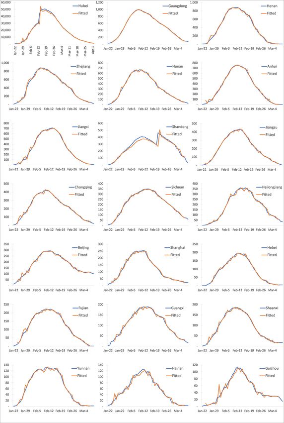
As can be seen from Figure 6, the regressions for ijt …t reasonably well and trace the epidemic
curves accurately for all 21 Chinese provinces that we consider. Here, it is also notable that the time
to the peak of the epidemic curve is about 4 weeks for most provinces, and the time to completion is
biased upward due to the long delay (4 weeks or more) between infection and death.
12
The …gures in brackets are standard errors of the estimates.
24around 8 weeks. It is clear that epidemic curves this ‡at could not have materialized if it were not
for the very stringent social distancing policies implemented by the Chinese authorities, as re‡ected
in the very low estimates of j that we obtain, particularly once we consider provinces outside of
the epicenter of the epidemic.
Thus far, we have focussed on Chinese data since they represent completed epidemic cycles
across all 21 provinces. In contrast, at the time of writing, the peak of the epidemic has not been
reached for other countries, where the …rst reported cases came a few weeks after China. So we
now turn our attention to other countries, considering only those countries for which we have a
su¢ cient history for a reliable estimation of . Before proceeding, for an accurate comparison with
China, we report estimates of and for the same 22 Chinese provinces over a subsample ending
on 20th of February (covering the initial stages of the epidemic before reaching its peak). For this
subsample the estimates of (and ) are summarized in Table 4, which are directly comparable to
the full-sample estimates in Table 2. As can be seen, for we obtain much smaller estimates when
we use the subsample as compared to the full sample, with a mean estimate of 0:018 compared to
the full-sample estimate of 0:046, possibly re‡ecting the fact that before the peak of the epidemic
the data do not capture the recoveries and deaths that will materialize in the following three weeks.
It is therefore reasonable to expect that removal rates in other countries will converge to the very
precise estimates for China that we have already reported for the full sample in Table 2.
Subsample estimates of are presented in Table 3. For the point estimates based on the
two samples are very close, in line with the news reporting/anecdotal evidence of stringent and
consistent implementation of social distancing. Remarkably, these estimates continue to be very
precisely estimated. A visual comparison between the estimates of based on the full and the
subsamples is given in Figure 7. As can be seen, the estimates of are essentially the same for the
two sample periods, with the exception of the estimates for Shandong province where the subsample
estimate of is larger than the full-sample estimate. This could be due to the fact that outside the
epicenter, Shandong is the only province to experience a second wave in mid course, as is evident
from the plot of active cases for Shandong in Figure 6.
25Table 2: Estimates of the recovery rates ( j ) for Chinese provinces
^j (s.e.) ^j (s.e.) ^j
Hubei 0.035 (0.0030) 1.0088 (0.0018) 0.09
Guangdong 0.042 (0.0032) 1.0070 (0.0018) 0.08
Henan 0.054 (0.0054) 1.0072 (0.0025) 0.08
Zhejiang 0.044 (0.0038) 1.0073 (0.0019) 0.09
Hunan 0.056 (0.0039) 1.0055 (0.0017) 0.07
Anhui 0.049 (0.0052) 1.0081 (0.0026) 0.09
Jiangxi 0.047 (0.0049) 1.0081 (0.0025) 0.09
Shandong 0.046 (0.0060) 1.0084 (0.0030) 0.09
Jiangsu 0.055 (0.0045) 1.0063 (0.0021) 0.08
Chongqing 0.043 (0.0039) 1.0077 (0.0021) 0.09
Sichuan 0.040 (0.0034) 1.0081 (0.0019) 0.09
Heilongjiang 0.043 (0.0052) 1.0086 (0.0030) 0.09
Beijing 0.033 (0.0042) 1.0053 (0.0028) 0.07
Shanghai 0.043 (0.0065) 1.0034 (0.0034) 0.06
Hebei 0.066 (0.0058) 1.0060 (0.0023) 0.08
Fujian 0.039 (0.0051) 1.0078 (0.0029) 0.09
Guangxi 0.037 (0.0051) 1.0093 (0.0031) 0.10
Shaanxi 0.044 (0.0051) 1.0074 (0.0027) 0.09
Yunnan 0.041 (0.0068) 1.0085 (0.0038) 0.09
Hainan 0.052 (0.0078) 1.0080 (0.0037) 0.09
Guizhou 0.056 (0.0079) 1.0049 (0.0038) 0.07
MG estimates 0.046 (0.0017) 1.0072 (0.0003) 0.08
q
Notes: Estimation is based on regression rj;t+1 = j rjt + j j ijt + "j;t+1 , where j = ln( j ). See also (27). Sample is
Jan-22 to March-31, 2020 (T = 70) with the exception of Hubei which is estimated using the sample Jan-22 to Apr-6 (T = 76).
26Table 3: Estimates of exposure rates ( j ) per 100,000 population for Chinese provinces
( = 0:5, R0 = 3)
Using province-speci…c estimates ^j ,^ j Using pooled estimates ^M G ; ^ M G
Full sample Subsample Full sample Subsample
cj (s.e.) cj (s.e.) cj (s.e.) cj (s.e.)
Guangdong 0.441 (0.042) 0.431 (0.044) 0.491 (0.044) 0.484 (0.046)
Henan 0.610 (0.099) 0.571 (0.115) 0.501 (0.085) 0.457 (0.093)
Zhejiang 0.610 (0.079) 0.599 (0.110) 0.643 (0.084) 0.633 (0.117)
Hunan 0.663 (0.108) 0.677 (0.146) 0.468 (0.072) 0.472 (0.095)
Anhui 0.734 (0.159) 0.692 (0.157) 0.722 (0.168) 0.675 (0.164)
Jiangxi 0.846 (0.166) 0.770 (0.176) 0.868 (0.180) 0.786 (0.190)
Shandong 0.087 (0.008) 0.200 (0.034) 0.088 (0.008) 0.216 (0.040)
Jiangsu 0.389 (0.065) 0.399 (0.075) 0.297 (0.049) 0.300 (0.057)
Chongqing 0.586 (0.106) 0.583 (0.133) 0.644 (0.118) 0.642 (0.150)
Sichuan 0.166 (0.021) 0.165 (0.026) 0.211 (0.027) 0.213 (0.035)
Heilongjiang 0.364 (0.050) 0.364 (0.057) 0.414 (0.060) 0.420 (0.072)
Beijing 0.412 (0.077) 0.444 (0.127) 0.586 (0.096) 0.644 (0.163)
Shanghai 0.498 (0.106) 0.524 (0.156) 0.451 (0.079) 0.472 (0.115)
Hebei 0.215 (0.050) 0.205 (0.070) 0.126 (0.029) 0.115 (0.037)
Fujian 0.211 (0.042) 0.194 (0.041) 0.266 (0.053) 0.251 (0.054)
Guangxi 0.106 (0.030) 0.104 (0.045) 0.156 (0.049) 0.156 (0.076)
Shaanxi 0.213 (0.040) 0.199 (0.050) 0.227 (0.043) 0.213 (0.054)
Yunnan 0.108 (0.020) 0.095 (0.019) 0.130 (0.026) 0.116 (0.025)
Hainan 0.461 (0.079) 0.463 (0.108) 0.396 (0.069) 0.395 (0.094)
Guizhou 0.131 (0.034) 0.133 (0.046) 0.096 (0.023) 0.096 (0.031)
MG estimate 0.393 (0.050) 0.391 (0.047) 0.389 (0.050) 0.388 (0.047)
Hubei 16.306 (1.764) 16.164 (2.765) 23.743 (2.720) 23.584 (4.395)
h i
j R0
Notes: Estimation is based on regressions ij;t+1 = i2jt =ij;t 1
3
j + 2
j ijt ij;t 1 1 j
2
j ijt + jt+1 , for
j
j = 1; 2; :::; 21 (provinces), with j; j imposed equal to the country-speci…c estimates from Table 2 or their MG estimates
from Table 2. The full sample is the same as in Table 2. The subample is Jan-22 to Feb-20 (T = 30).
27You can also read