Understanding deep learning in land use classification based on Sentinel 2 time series - Nature
←
→
Page content transcription
If your browser does not render page correctly, please read the page content below
www.nature.com/scientificreports
OPEN Understanding deep learning
in land use classification based
on Sentinel‑2 time series
Manuel Campos‑Taberner1*, Francisco Javier García‑Haro1, Beatriz Martínez1,
Emma Izquierdo‑Verdiguier2, Clement Atzberger2, Gustau Camps‑Valls3 &
María Amparo Gilabert1
The use of deep learning (DL) approaches for the analysis of remote sensing (RS) data is rapidly
increasing. DL techniques have provided excellent results in applications ranging from parameter
estimation to image classification and anomaly detection. Although the vast majority of studies report
precision indicators, there is a lack of studies dealing with the interpretability of the predictions. This
shortcoming hampers a wider adoption of DL approaches by a wider users community, as model’s
decisions are not accountable. In applications that involve the management of public budgets or
policy compliance, a better interpretability of predictions is strictly required. This work aims to deepen
the understanding of a recurrent neural network for land use classification based on Sentinel-2 time
series in the context of the European Common Agricultural Policy (CAP). This permits to address
the relevance of predictors in the classification process leading to an improved understanding of
the behaviour of the network. The conducted analysis demonstrates that the red and near infrared
Sentinel-2 bands convey the most useful information. With respect to the temporal information, the
features derived from summer acquisitions were the most influential. These results contribute to the
understanding of models used for decision making in the CAP to accomplish the European Green Deal
(EGD) designed in order to counteract climate change, to protect biodiversity and ecosystems, and to
ensure a fair economic return for farmers.
The European Commision (EC) recently proposed the Resource-efficient Europe initiative1 under the Europe
2020 strategy for a sustainable growth via a resource-efficient, and low-carbon economy. In this aspect, the EC
adopted also a new regulation for the Common Agricultural Policy (CAP) that promotes the use of remote sens-
ing (RS) data for monitoring parcels, evaluates cross-compliance and eventually provides subsidy payments to
farmers2. The basic payment aims at avoiding the abandonment of agricultural parcels. The green direct payment,
also known as “greening”, supports farmers who undertake agricultural practices that benefit the environment and
meet climate objectives. In particular they should diversify crops, maintain grasslands, and allocate 5% of arable
land to areas that improve biodiversity. To put this in context, in 2018 a total of 73.7 million Euros were paid to
farmers in the Valencian Community (Spain) whereof 18.8 million and 9.6 million were dedicated to the basic
and greening payments, respectively. These actions are supported by land use classifications obtained from RS
data. This requires on one hand a good crop identification, and on the other hand classification interpretability,
which is key to provide fair assignments.
The categorisation of remotely-sensed images is usually achieved using machine learning algorithms, being
deep learning (DL) the most accurate paradigm. DL has recently raised up as a discipline used in RS and Earth
sciences3. A variety of geoscience topics dealing with extreme weather patterns4, climate change projections5,
precipitation nowcasting6, and carbon fluxes p rediction7 can be found in the literature. There is also a wide range
of RS topics such as image f usion and r egistration9, change d
8
etection10, image s egmentation11, and (drought)
forecasting12 that involve DL methods. Nonetheless, the vast majority of RS studies dealing with DL techniques
are dedicated to classification including scene identification, land use and land cover (LULC) classification, and
object detection13–18.
1
Environmental Remote Sensing group (UV‑ERS), Universitat de València, 46100 Burjassot, Valencia,
Spain. 2Institute of Geomatics, University of Natural Resources and Life Sciences, Vienna (BOKU), Peter Jordan
Str. 82, 1190 Vienna, Austria. 3Image Processing Laboratory (IPL), Universitat de València, 46980 Paterna,
Spain. *email: manuel.campos@uv.es
Scientific Reports | (2020) 10:17188 | https://doi.org/10.1038/s41598-020-74215-5 1
Vol.:(0123456789)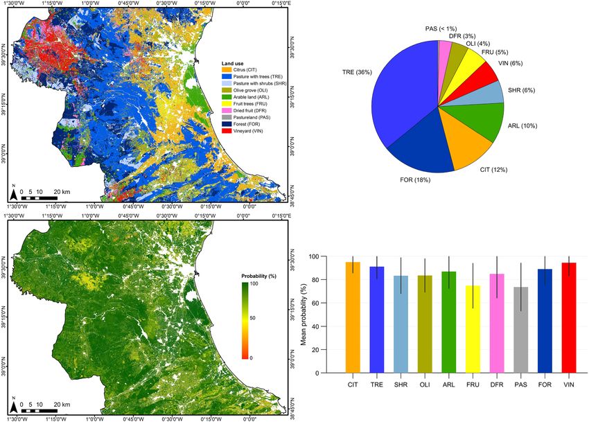
www.nature.com/scientificreports/
Figure 1. Scheme of the proposed approach for deepen understanding of a recurrent neural network for land
use classification based on remote sensing data in the context of the European Common Agricultural Policy
(CAP).
RS classification approaches mainly exploit information derived from the spatial and spectral domains of a
single image, and also the temporal information in the case of using image time series. DL classification algo-
rithms that use RS data can be roughly differentiated in two major groups: techniques that design convolutional
neural networks (CNNs) architectures for spatial learning, and recurrent neural networks (RNNs) for sequential
learning. For a comprehensive overview, we refer the reader to excellent reviews of DL techniques and applica-
tions in RS provided by Zhang et al.19, Zhu et al.20, and Ma et al.21. CNNs are composed of multiple layers that
are the result of performing spatial convolutions typically followed by activation units and pooling. RNNs are
able to deal with sequences of data (e.g., RS time series), in such a way that the output from the previous time
step is fed as input to the current step. However, RNNs suffer the vanishing gradient problem, which may lead
to stop the network from further training22. Long short-term memory (LSTM) networks are a particular type
of RNNs that mitigate the vanishing gradient problem since they employ a forget gate that varies at every time
step and decides what information is retained and forgotten/erased23.
DL approaches usually outperform other (shallow) machine learning techniques in terms of overall accuracy
(OA)24–26. However, the understanding of these techniques is limited27, and typically, the better the learning of an
algorithm the more difficult its interpretation i s28. This lack of interpretability is a major point to consider when
using these algorithms. For many users it is not only important to use an algorithm that provides high accuracy
but also to know how the algorithm is reaching the provided predictions29. The interpretability of predictions
becomes a critical aspect when they are used as rationale for decision making, such as in medicine, business or
in the banking/payment s ector30–32.
Recently, some approaches have been proposed to evaluate the interpretability of deep learning m odels33,34
including methods based on model decomposition, sensitivity analysis, and feature visualisation. The relevance of
network inputs can for example be obtained by the gradient-based sensitivity analysis (GBSA), which computes
the prediction function squared partial derivatives with a standard gradient b ackpropagation35. The Layer-wise
Relevance Propagation (LRP)36 propagates the prediction backward in the neural network using propagation
rules until the input features are reached. Arras et al.37 proposed a LRP for LSTM networks that provided better
results than the GBSA on a five-class prediction task. Class activation maps were used to point out the most
discriminative regions used by a CNN to identify a c lass38.
In the field of RS there is a lack of studies that have delved into the interpretability of DL outputs. Wolanin
et al.39 derived regression activation maps providing information about predictions (crop yield) also retaining
the correspondence with the inputs (meteorological and satellite data). Marcos et al.40 provided Semantically
Interpretable Activation Maps (SIAM) indicating the presence of predefined attributes at different locations of
an image. Pelletier et al.41. developed a temporal CNN applying convolutions in the temporal domain in order to
quantitatively and qualitatively evaluate the contribution of network for crop mapping, as compared to RF and
bi-directional RNNs with stacks of Gated Recurrent Units (GRUs). Rußwurm and Körner42 proposed an encoder
structure with convolutional recurrent layers, and visualised internal activations over a sequence of cloudy and
non-cloudy Sentinel-2 images for crop classification. It is worth mentioning that a procedure used for improv-
ing the performance of RNNs is the attention mechanism (AM). AM implements a coding-decoding model for
identifying network key f eatures43,44. AM has been applied in different topics such as time travel p rediction45 or
46
text classification . In remote sensing and image processing AM has been used for improving classification in
very high-resolution i mages47,48 as well as to capture the spatial and channel d ependencies49. In this context, this
work aims at evaluating the interpretability of a DL algorithm based on a 2-layer bi-directional Long Short-Term
Memory network (2-BiLSTM) for land use classification over the province of València (Spain) in the framework
of CAP activities (Fig. 1 shows an scheme of the process). Sentinel-2 time series during the 2017/2018 agronomic
year were used as inputs for the classification. The influence of the various spectral and temporal features on
the classification accuracy was assessed by means of an added-noise permutation approach in both temporal
and spectral domains. The network temporal predictive behaviour was explained for every date throughout the
agronomic year. In addition, different network architectures were designed and assessed, and a comparison in
terms of accuracy with a set of widely used machine learning algorithms has been carried out.
Scientific Reports | (2020) 10:17188 | https://doi.org/10.1038/s41598-020-74215-5 2
Vol:.(1234567890)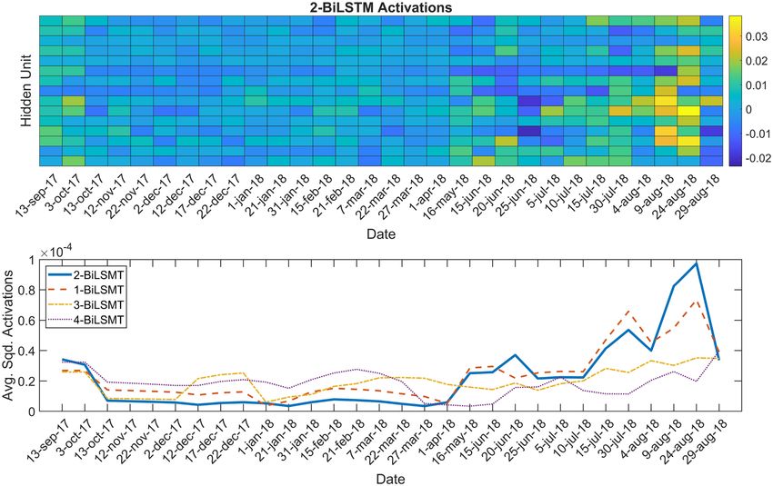
www.nature.com/scientificreports/
Figure 2. Classification map derived using the 2-BiLSTM model and the associated spatial distribution (up),
and the pixel probability map and associated class mean probabilities (bottom). For the sake of visualisation,
parcels belonging to rice, fallow, barley, oat, wheat, sunflower, and triticale have been grouped and displayed as
arable land (ARL). Non interest areas have been masked out. Error bars indicate the standard deviation of every
class probability. The maps were generated with the Arcmap v.10.5 software (https://desktop.arcgis.com/es/
arcmap/).
Results
Figure 2 shows the classification map obtained in the area using the 2-BiLSTM model. The derived classification
map exhibits a spatial distribution of classes in accordance with the Land Parcel Identification System (LPIS) of
Spain also known as Sistema de Información Geográfica de Parcelas Agrícolas (SIGPAC)50, namely: fruit trees
and citrus crops in coastal zones, arable lands in the west belonging to diverse cereal crops, and rice crops in
the east nearby the Albufera Natural, and natural vegetation, dried fruits, and vineyards mainly in inland zones.
The 60% of the area is classified as natural vegetation (TRE, FOR, SHR, and PAS) (see Fig. 2), whereas the 24%
is occupied by permanent crops (DFR, FRU, CIT, OLI), and the remaining 16% is classified as annual crops
including vineyards (VIN) and arable lands (ARL) that comprises rice, fallow, barley, oat, wheat, sunflower,
and triticale. Figure 2 (bottom) shows the probability map with which every pixel is classified by the 2-BiLSTM
network. All classes reported a mean probability ≥ 83% except FRU and PAS in which the mean probability
was 73%, and 72%, respectively. The vast majority of the area was classified with a high level of confidence (see
greenish areas in Fig. 2, bottom). However, there exist low confidence zones (red pixels) in which the classifica-
tions should be taken carefully.
The proposed 2-BiLSMT network yielded an overall accuracy (OA) of 98.7% over the test set that was never
used in the training. This accuracy outperformed the ones obtained by the rest of BiLSTM architectures as well as
other classification algorithms (see Table S1 in Supplementary information). It is worth mentioning that in order
to identify possible spatial bias in the classification results, different random selections of the train/test sets (pre-
serving the 70%/30% proportion) both at pixel and parcel-based approaches were conducted, and no significant
changes in performance were obtained for all the evaluated methods. The 2-BiLSTM network performed well
over all classes. The confusion matrix obtained with the 2-BiLSTM (see Fig. S1 in Supplementary information)
highlights the great precision of the classification algorithm over all classes. Table 1 shows the precision, recall,
and F-1 score obtained for every class. The best precision was achieved over rice fields (99.9% in both user and
producer accuracy) whereas the lowest one was obtained over fruit trees with a 7.4% and 8.6% of predicted, and
true negative rates, respectively (see Fig. S1 in Supplementary information). The 2-BiLSTM network classified
Scientific Reports | (2020) 10:17188 | https://doi.org/10.1038/s41598-020-74215-5 3
Vol.:(0123456789)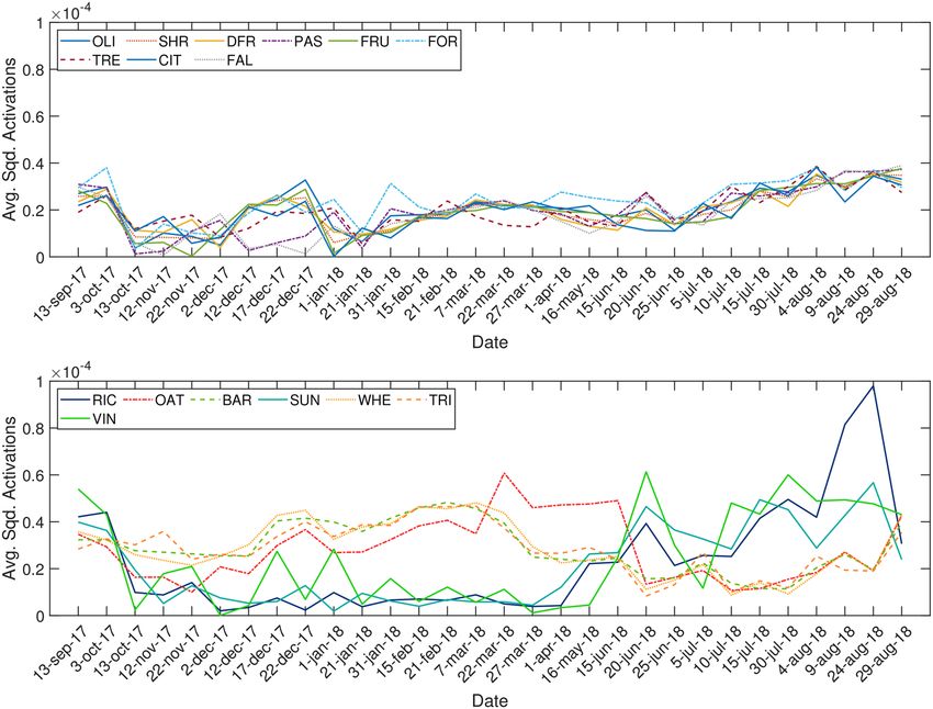
www.nature.com/scientificreports/
Class Precision (%) Recall (%) F-1 score (%)
RIC 99.9 99.9 99.9
FOR 99.7 99.8 99.7
TRE 99.4 99.5 99.4
PAS 98.9 97.5 98.2
SHR 98.8 98.9 98.8
WHE 98.5 97.6 98.0
VIN 98.2 98.5 98.3
CIT 97.9 98.4 98.1
TRI 97.9 97.6 97.7
BAR 97.7 97.4 97.5
DFR 97.0 97.8 97.4
FAL 95.8 94.6 95.2
OAT 95.4 94.4 94.9
SUN 94.4 94.0 94.2
OLI 93.9 91.1 92.5
FRU 92.6 91.4 92.0
Table 1. Performance (precision, recall, and F-1 score) of every class obtained with the 2-BiLSTM network
over the validation set.
all classes with an accuracy ≥ 91.4% in precision, recall, and F-1 score. The 2-BiLSTM network performed also
excellent over natural vegetation such as forest (FOR), and pasture with trees (TRE) classes, revealing precision,
recall and F-1 score ≥ 99% (see Table 1). Permanent crops such as fruit trees (FRU), and citrus (CIT) were more
difficult to distinguish between them (see Fig. in Supplementary information). The same applies to vineyard
(VIN), olive grove (OLI), and dried fruits (DFR), in which greater confusion is reported by the confusion matrix
(see Fig. S1 in Supplementary information). The discriminatory power of the classifier among classes belonging
to permanent crops is slightly lower if compared with the annual crops. This is mainly due to that differences in
the temporal remotely sensed signal on permanent crops is lower than the ones on annual crops in which the
phenological development influences more on temporal changes in reflectance.
The relevance of every Sentinel-2 date, and derived predictors in the 2-BiLSTM model is exhibited in Fig. 3.
Across the temporal domain, the information provided by the Sentinel-2 image acquired on August 9th, 2018
was the most relevant, while the relevance of the image acquired on December 17th, 2018 is ≈ 66% lower. The
NDVI temporal sequence is the most relevant predictor used by the 2-BiLSTM network. On the contrary, the
Sentinel-2 aerosols band (B1) provides the least-used information by the network (≈ 90% lower compared to
NDVI). The relevance provided by the 2-BiLSTM model was compared with the one provided by RF classifier.
The most important attributes for making the RF predictions were the NDVI of differente dates, as well as the
entropy of NDVI, and the red and nir channels (see Fig. S2 in Supplementary information). This is in accord-
ance with the results provided by the 2-BiLSTM network. However, RF seems not to be aware of the temporal
information since the most relevant predictors belong to disjointed dates in terms of classes’ phenology.
The temporal predictive performance of the 2-BiLSTM network over two correctly classified pixels (one for
natural vegetation, and one for crops) is shown in Fig. 4 in order to understand how the classifications are finally
obtained. Over a pixel located within an homogeneous rice field (Fig. 4, left), the rice classification probability
(purple line) presents the lowest values during the pre-sowing (winter–spring) period. During this time, the per
class probabilities of all classes are similarly low. There is a sharp increase in the probability from the beginning
of the rice c ycle51,52 (mid-may) until the full development/maturity in august, reaching a maximum (100% prob-
ability) from the period from senescence to the end of autumn. In the case of a pixel located within a pasture
with shrubs (SHR) site (Fig. 4, right), the SHR classification probability (orange line) shows high values almost
over the entire period, and in particular during winter–spring when crops do not ‘interfere’ in the classification.
However, even though the final classification is correctly assigned to SHR, there is a non-negligible probability
assigned to the class pasture with trees (TRE) that is sometimes higher than the SHR probability. This is partly
due to the spectral similarity between classes.
The 2-BiLSTM network most activated hidden units are shown in the heatmap displayed in Fig. 5 (top). The
greenish and yellowish tones which pop-up, belong to the most activated hidden units, and generally correspond
to summer acquisitions. To better quantify the activations along dates, Fig. 5 (bottom) shows the mean squared
activations in the temporal domain of all considered BiLSTM architectures. The 2-BiLSTM and 1-BiLSTM
networks present a similar behaviour with higher activations in summer. However the 3-BiLSTM, and specially
the 4-BiLSTM network reveal more homogeneous activations along dates. Figure 6 (top) shows the activations
of land uses belonging to natural vegetation (SHR, PAS, FOR, TRE, and FAL), and permanent crops (OLI, DFR,
FRU, CIT). These classes present similar activations along time. Regarding annual crops, the activations are
higher during the main phenological activity of each class (Fig. 6, bottom). For example, RIC, VIN, and SUN
crops show higher activations during summer dates, whereas OAT, BAR, WHE and TRI activations are higher
in winter–spring according to their phenological behaviour in the area.
Scientific Reports | (2020) 10:17188 | https://doi.org/10.1038/s41598-020-74215-5 4
Vol:.(1234567890)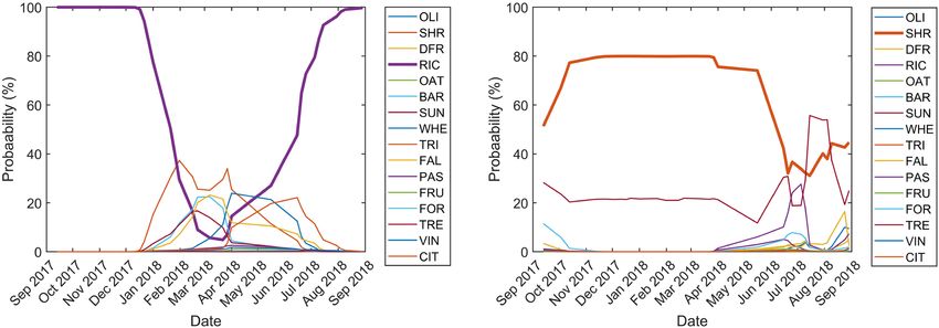
www.nature.com/scientificreports/
Figure 3. Relevance of every date (top) and predictor (bottom) in the 2-BiLSTM network.
Figure 4. Probability evolution along time steps for representative rice (left) and pasture with shrubs (right)
pixels.
Discussion
Differentiating and identifying vegetation types with high level of confidence using RS data is possible if long
enough time series of images are a vailable53,54. In addition, a high temporal frequency is required to cover and
characterize crop-specific phenological cycles, and to benefit from the differences established between the dif-
ferent classes along time. The high spatial–temporal resolution of the Sentinel-2 constellation, consisting of two
identical satellites with 13 spectral bands and a combined revisit frequency of maximum 5 days, is especially
well suited for identifying vegetation types and for studying vegetation dynamics.
In RS image classification, exploiting the temporal domain with RNNs is of paramount relevance. Conven-
tional RNNs, however, present instabilities and problems during the training phase because backpropagated
gradients tend to fade over time, which produces difficulties with learning long-term dependencies. LSTM
networks mitigate this by incorporating a series of steps to decide which information is going to be stored
(“memorized”), and which deleted (“forgotten”). Thus, the network has a certain “memory”. Furthermore, if the
Scientific Reports | (2020) 10:17188 | https://doi.org/10.1038/s41598-020-74215-5 5
Vol.:(0123456789)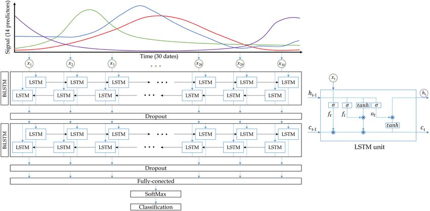
www.nature.com/scientificreports/

                                            Figure 5.  Heatmap of the 2-BiLSTM activations for every date (top), and mean squared activations in the
                                            temporal domain for the four considered BiLSTM architectures (bottom).

                                            Figure 6.  Activations observed in the 2-BiLSTM network for (top) natural vegetation and permanent crops,
                                            and (bottom) annual crops.

          Scientific Reports |   (2020) 10:17188 |              https://doi.org/10.1038/s41598-020-74215-5                                              6

Vol:.(1234567890)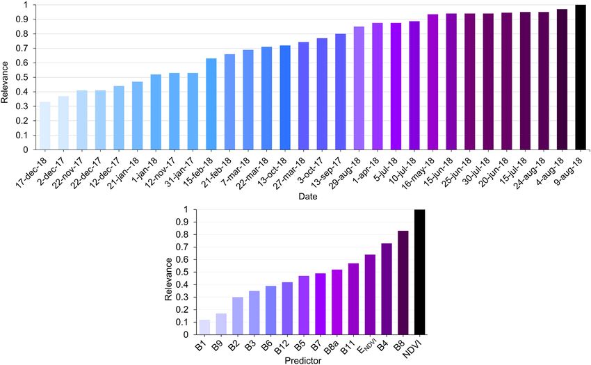
www.nature.com/scientificreports/
memory provides information on both past and future states as in the case of BiLSTMs, its use in applications
where it is convenient to learn from the whole time series is of special interest.
When classifications are to be used for decision making such as the CAP, it is convenient not only to report
results in terms of accuracy, but also to provide an explanation of what is internally happening in the classifier
in order to subsequently interpret and explain the results. This lacking assessment is one of the main challenges
DL algorithms are currently facing, since these algorithms are often seen as “black boxes” that perform high
accuracy classifications without the operator being able to interpret what is happening in the algorithm. In this
regard, the proposed procedure for evaluating the comprehensibility of the network revealed that the network
mainly extracts information from the temporal evolution of the NDVI, the near-infrared (B8) and red (B4)
bands, and the spatial information provided by ENDVI . This aspect confirms the relevance of the Sentinel-2 near
infrared, and red bands to categorise vegetation, as these two bands well address differences in leaf area index
(LAI) and leaf pigmentation, respectively52. In a similar way, the fact that Band 11 (SWIR) also scored relatively
high underlines the effectiveness of the proposed scheme, as this band is known for providing independent
information related to crop water and/or protein c ontent55. Several recent studies using Sentinel-2 data have
highlighted the importance of this band for crop type identification50,56.
According to the per date relevance analysis, the network mainly uses the information from the Sentinel-2
images acquired in summer, which is consistent with the phenological activity of most of the classes identi-
fied in the study area. Likewise, it is plausible that the winter period does not offer many clues for crop type
identification.
The classification results confirm that the use of two BiLSTM layers improves the OA compared to the rest
of evaluated classifiers (see Table S1 in Supplementary information). The highest precision was obtained on rice
crops (RIC) where practically all the pixels are correctly classified thanks to its unique crop cycle and planting
pattern. This result highlights the usefulness of Sentinel-2 multitemporal data for characterizing rice as also
reported in other s tudies50. Regarding the architecture of the recurring networks, the 2-BiLSTM network pro-
duced the best results. It is worth mentioning that the increase of the number of layers in a deep neural network
does not necessarily lead to better classification results. In fact, the results show a clear decreasing accuracy in
the case of 4-BiLSMT, which is even outperformed by the RF algorithm. This is partly because in multi-layered
architectures, even though dropout layers are used, networks may tend to overfit and lose generalisation power
thus decreasing accuracy. In addition, the vanishing gradient problem may also persist in architectures made by
high number of layers. In the case of the 4-BiLSTM network we also found that the activations are quite similar
along dates, which means there is no clearly relevant period used by the network.
The results on the temporal predictive performance of the 2-BiLSTM network reveals how the network
adapts both the per class probability and the classifications along time steps. The activation of the hidden units
reveal how the information is flowing through the network. Results showed that the most activated units belong
to summer dates. This means that the network is giving more importance to those dates since the wealth of
information is higher. This result goes in line with the results obtained in the added-noise permutation results.
Conclusions
The use of satellite observations for land use identification and monitoring is one of the CAP strategies that are
in line with the Green Deal’s ambitions. These remote sensing-based controls can be used in the administrative
process associated to direct and greening payments compliance. Possible inconsistencies between parcel classi-
fications and farmers declarations should be clarified by in situ checks. In the case of farmers who do not respect
greening rules, this may lead paying agencies to impose proportionate sanctions (depending on the scope of
the non-compliance and severity) on top of the reduction in greening payments. Therefore, the use of accurate
models—and explainable and interpretable—predictions is fundamental in these applications.
The performance of a deep recurrent network was assessed for land use classification from time series of
Sentinel-2 data. The overall accuracy reached by the 2-BiLSTM network was 98.7%, outperforming the rest of
the classification algorithms evaluated. The obtained accuracy was ≥ 91.4% in all cases, which highlights the
algorithm robustness, and it excelled reaching to 99.9% over rice crops. Even though the per class accuracy were
high, some confusion was also reported mainly over permanent crops.
The best results were achieved using two BiLSTM layers, which indicates that increasing layers is not syn-
onymous to better performance in deep learning approaches. The most relevant information used by the net-
work during training is extracted from the NDVI, B8 (NIR), B4 (red) and ENDVI predictors. From the temporal
standpoint the Sentinel-2 images corresponding to the summer period were the most informative. The network’s
outputs interpretability assessment exposed the information flow through the network also evidencing the dates
in which higher activations of the hidden units were produced.
These analyses help to understand the behaviour of deep learning models in agricultural applications. In par-
ticular, in the CAP activities in which payments to farmers must be well-founded, the use of classification models
providing explainable predictions are of great interest. The conducted work not only confirm well established
knowledge in remote sensing science but also opens the door to new studies in the field of the comprehensibility
of deep learning algorithms in agricultural and environmental applications.
Materials and methods
Sentinel‑2 time series. The European Space Agency (ESA) provides free access to Copernicus Sentinel-2
data from the Sentinels Scientific Data Hub (SSDH). Sentinel-2 mission is composed of two twin satellites (Sen-
tinel-2A and Sentinel-2B) that combined, offer a 5-day period of revisit. Both platforms carry on board the
MultiSpectral Imager (MSI) sensor that provides multispectral images in 13 spectral bands covering areas of the
visible spectrum, near infrared, and short-wave infrared. The spatial resolution of the data varies depending on
Scientific Reports | (2020) 10:17188 | https://doi.org/10.1038/s41598-020-74215-5 7
Vol.:(0123456789)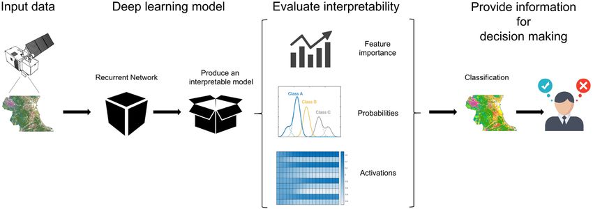
www.nature.com/scientificreports/
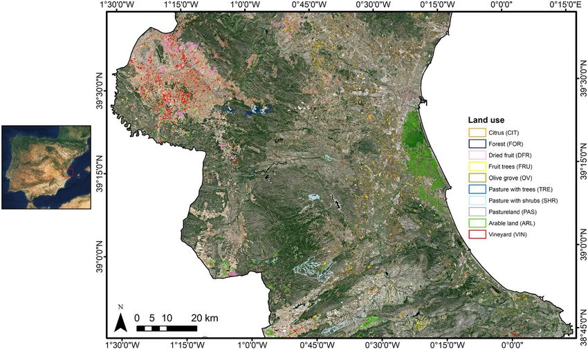
Figure 7. Location of the study area (eastern Spain), and a corresponding Sentinel-2 RGB (B4, B3, B2)
composite image acquired on September 13, 2017 with overlaid ground truth. For the sake of visualisation,
parcels belonging to rice, fallow, barley, oat, wheat, sunflower, and triticale have been grouped and displayed as
arable land (ARL). The maps were generated with the Arcmap v.10.5 software (https://desktop.arcgis.com/es/
arcmap/).
the band: the B2 (blue channel), B3 (green channel), B4 (red channel), and B8 (near infrared channel) bands are
provided at 10 m; the red-edge bands (B5, B6, B7), the B8a (narrow-near-infrared channel) band, and the short-
wave infrared bands (B11 and B12) are provided at 20 m; the B1 (aerosols), B9 (water vapour) and B10 (cirrus)
bands are available at 60 m of spatial resolution. The latter is usually used only for atmospheric correction.
Time series of Sentinel-2 data were downloaded from the SSDH covering the 2017/2018 agronomic year from
September, 2017 to August, 2018. Since the Valencia province lies on two Sentinel-2 tiles (T30SYJ and T30SXJ),
a total of 60 (30 per tile) cloud free images were identified and downloaded over the Valencia province. The
Sentinel-2 level 2A product that provides surface reflectance in twelve bands (all except B10) was downloaded.
The 20 m and 60 m spatial resolution bands were resampled to 10 m in order to obtain a data set of 10 m in the
all twelve bands. Figure 7 shows the location of the study area in Spain, and a 10 m Sentinel-2 RGB (B4, B3, B2)
composite image over the area.
In addition to the twelve bands per image, the normalised difference vegetation i ndex57,58 (NDVI) computed
as NDVI = B8+B4
B8−B4
, and its entropy (ENDVI ) were calculated. The use of vegetation indices, and spatial information
such as textures, is a common procedure in RS to differentiate c lasses50,59,60. Altogether, time series of 14 features
along 30 time steps were used as predictors/inputs in the classification algorithms.
Ground data. The samples used for training and testing the classification models were provided by the
Department of Agriculture, Rural Development, Climate Emergency and Ecology Transition (http://www.agroa
mbient.gva.es/) belonging to the regional government of Valencia in Spain. This information comes from Valen-
cia’s province-wide in situ checks carried out during the 2017/2018 agronomic year. Sixteen land uses were cat-
egorised as pasture with trees (TRE), forest (FOR), vineyard (VIN), rice (RIC), pasture with shrubs (SHR), dried
fruit (DFR), citrus (CIT), fallow (FAL), barley (BAR), olive grove (OLI), pastureland (PAS), fruit trees (FRU),
oat (OAT), wheat (WHE), sunflower (SUN), and triticale (TRI). Table 2 shows the number of samples for every
class categorised in the field inspections. The data were geolocated over the Sentinel-2 images to match every
sample with its corresponding remote sensing sequence of data. Finally, 70% of the data were used for training
the algorithms whereas the remaining 30% were used only for validation.
Bi‑directional long short‑term memory network (BiLSTM). LSTM is a special recurrent hidden unit
that was proposed to deal with the vanishing gradient problem in RNNs and learn long-term d ependencies23.
Recurrent networks based on LSTM units overcome this drawback by using a gate that controls whether the
incoming information is useful or not. Temporal dependencies are taken into account via what is known as the
network memory or memory cell. This information flows through each of the network LSTM units, which are
composed by three gates: the input (it ), forget (ft ), and output (ot ) gates. In a time step or instant t, the LSTM
Scientific Reports | (2020) 10:17188 | https://doi.org/10.1038/s41598-020-74215-5 8
Vol:.(1234567890)www.nature.com/scientificreports/
Land use # samples
TRE 663,995
FOR 495,223
VIN 240,418
RIC 230,935
SHR 165,110
DFR 153,727
CIT 125,161
FAL 84,491
BAR 71,623
OLI 49,829
PAS 33,408
FRU 29,859
OAT 28,754
WHE 11,437
SUN 10,104
TRI 4252
TOTAL 2,398,326
Table 2. Number of pixels identified in the in situ visits. Of those, 70% were used for training and the
remaining 30% for validation.
unit reads the input xt , and the previous hidden state ht−1. Their combination is modulated by an hyperbolic
tangent as:
c̃t = tanh(Wc xt + Uc ht−1 + bc ), (1)
where Wc , Uc , and bc are the input weights, the recurrent weights, and the bias, respectively. The input gate
determines which information is stored in the memory cell by means of a sigmoid function:
it = σ (Wi xt + Ui ht−1 + bi ), (2)
and similarly, the forget gate decides which content of the existing memory cell is forgotten:
ft = σ (Wf xt + Uf ht−1 + bf ). (3)
The information is updated into the memory cell by adding the information coming from both the input and
forget gates, i.e., adding new information from ct , and rules out part of the current memory information:
ct = it ⊙ c̃t + ft ⊙ ct−1 (4)
Finally, the output (hidden) state is obtained by the output gate and the updated memory cell as:
ht = ot ⊙ tanh(ct ), (5)
where the output gate ot that determines the part of the memory content that will be revealed is given by:
ot = σ (Wo xt + Uo ht−1 + bo ). (6)
LSMT units can be combined to obtain a bi-directional long short-term memory (BiLSTM) network. The BiLSTM
networks are formed by two LSTM units per time step, and take into account not only past temporal dependences
but also information of future time states. Hence, BiLSTM networks learn from the complete time series at each
time step thus having a global view of the s equences61. In this work an deep network architecture composed by
a combination of two BiLSTM layers (2-BiLSTM) was used, as shown in Fig. 8. The main components of the
2-BiLSTM network are: (1) the input layer formed by the 14 Sentinel-2 selected time series, (2) two BiLSTM
layers with 100 hidden units followed by a 50% dropout layer to avoid overfitting, (3) a fully-connected layer
connecting the units to every activation unit of the next layer, (4) a softmax layer that computes the probability
of every class in the network output, and (5) the output layer containing the predictions.
Evaluation and interpretability. The accuracy of the proposed 2-BiLSTM network was assessed by com-
puting the overall accuracy in a first step. The obtained accuracy was compared with the ones obtained using
other network architectures, namely three similar networks formed by a single (BiLSTM), three (3-BiLSTM),
and four BiLSTM layers (4-BiLSTM), as well as with different machine learning classification algorithms: deci-
sion trees (DT), k-nearest neighbours (k-NN), neural networks, support vector machine (SVM), and random
forests (RF).
The 2-BiLSMT network behaviour was subsequently addressed by identifying the most relevant inputs (i.e.,
predictors) in the spectral and temporal domains. This was achieved by means of an added-noise permutation
Scientific Reports | (2020) 10:17188 | https://doi.org/10.1038/s41598-020-74215-5 9
Vol.:(0123456789)www.nature.com/scientificreports/
Figure 8. Architecture of the 2-BiLSMT network (left), and LSTM unit components (right). In our case, 14
features along 30 time steps were used as predictor variables.
approach consisting in the adding of Gaussian white noise N(0, σ 2 ), being σ 2 the 3% of the perturbed signal
amplitude. The noise was added to a single predictor in all time steps remaining the rest of the predictors
unperturbed. This process was repeated for every predictor, thereby obtaining different accuracies for every
case. The relevance of each predictor was computed as the difference between the accuracy obtained with no
perturbation and the obtained when the perturbation was applied. The results were normalised with respect
to the most relevant predictor. This approach was carried out again to identify the most relevant date. In this
case the perturbation was added to all predictors in a single time step leaving the rest of the dates unperturbed.
The interpretability of the classifications was addressed by showing how predictions and their probability
change between time steps. In addition, the BiLSTM hidden units activation was visualised, and the average
squared activations in the temporal domain were computed to analyse how the information flows through the
network.
Received: 20 July 2020; Accepted: 24 September 2020
References
1. Commission, E. et al. A resource-efficient Europe-flagship initiative under the Europe 2020 strategy. Communication 2011, 21
(2011).
2. Union, E. Commission implementing regulation (eu) 2018/746 of 18 May 2018 amending implementing regulation (eu) no
809/2014 as regards modification of single applications and payment claims and checks. Off. J. Eur. Union 61, 1–7 (2018).
3. Reichstein, M. et al. Deep learning and process understanding for data-driven earth system science. Nature 566, 195–204 (2019).
4. Liu, Y. et al. Application of deep convolutional neural networks for detecting extreme weather in climate datasets. arXiv: 1605.01156
(arXiv preprint) (2016).
5. Vandal, T. et al. Deepsd: Generating high resolution climate change projections through single image super-resolution. In Proceed-
ings of the 23rd ACM Sigkdd International Conference on Knowledge Discovery and Data Mining, 1663–1672 (2017).
6. Shi, X. et al. Deep learning for precipitation nowcasting: A benchmark and a new model. Adv. Neural Inf. Process. Syst. 20,
5617–5627 (2017).
7. Reichstein, M. et al. Potential of new machine learning methods for understanding long-term interannual variability of carbon
and energy fluxes and states from site to global scale. AGUFM 2016, B44A-07 (2016).
8. Liu, Y. et al. Deep learning for pixel-level image fusion: Recent advances and future prospects. Inf. Fusion 42, 158–173 (2018).
9. Wang, S. et al. A deep learning framework for remote sensing image registration. ISPRS J. Photogramm. Remote Sens. 145, 148–164
(2018).
10. Lyu, H., Lu, H. & Mou, L. Learning a transferable change rule from a recurrent neural network for land cover change detection.
Remote Sens. 8, 506 (2016).
11. Liu, Y., Minh Nguyen, D., Deligiannis, N., Ding, W. & Munteanu, A. Hourglass-shapenetwork based semantic segmentation for
high resolution aerial imagery. Remote Sens. 9, 522 (2017).
12. Lees, T. et al. A machine learning pipeline to predict vegetation health. Eighth International Conference on Learning Representations
1–5, (2020).
13. Zhao, W. & Du, S. Learning multiscale and deep representations for classifying remotely sensed imagery. ISPRS J. Photogramm.
Remote Sens. 113, 155–165 (2016).
14. Rußwurm, M. & Körner, M. Multi-temporal land cover classification with long short-term memory neural networks. Int. Arch.
Photogramm. Remote Sens. Spat.Inf. Sci. 42, 551 (2017).
Scientific Reports | (2020) 10:17188 | https://doi.org/10.1038/s41598-020-74215-5 10
Vol:.(1234567890)www.nature.com/scientificreports/
15. Chen, Y., Lin, Z., Zhao, X., Wang, G. & Gu, Y. Deep learning-based classification of hyperspectral data. IEEE J. Sel. Top. Appl. Earth
Observ. Remote Sens. 7, 2094–2107 (2014).
16. Li, W., Fu, H., Yu, L. & Cracknell, A. Deep learning based oil palm tree detection and counting for high-resolution remote sensing
images. Remote Sens. 9, 22 (2017).
17. Hu, F., Xia, G.-S., Hu, J. & Zhang, L. Transferring deep convolutional neural networks for the scene classification of high-resolution
remote sensing imagery. Remote Sens. 7, 14680–14707 (2015).
18. Liang, H. & Li, Q. Hyperspectral imagery classification using sparse representations of convolutional neural network features.
Remote Sens. 8, 99 (2016).
19. Zhang, L., Zhang, L. & Du, B. Deep learning for remote sensing data: A technical tutorial on the state of the art. IEEE Geosci.
Remote Sens.Mag. 4, 22–40 (2016).
20. Zhu, X. X. et al. Deep learning in remote sensing: A comprehensive review and list of resources. IEEE Geosci. Remote Sens.Mag.
5, 8–36 (2017).
21. Ma, L. et al. Deep learning in remote sensing applications: A meta-analysis and review. ISPRS J. Photogramm. Remote Sens. 152,
166–177 (2019).
22. Goodfellow, I., Bengio, Y. & Courville, A. Deep Learning (The MIT Press, New York, 2016).
23. Hochreiter, S. & Schmidhuber, J. Long short-term memory. Neural Comput. 9, 1735–1780 (1997).
24. Campos-Taberner, M. et al. Processing of extremely high-resolution lidar and RGB data: Outcome of the 2015 IEEE GRSS data
fusion contest-part a: 2-d contest. IEEE J. Sel. Top. Appl. Earth Observ. Remote Sens. 9, 5547–5559 (2016).
25. Zhong, L., Hu, L. & Zhou, H. Deep learning based multi-temporal crop classification. Remote Sens. Environ. 221, 430–443 (2019).
26. Liu, T., Abd-Elrahman, A., Morton, J. & Wilhelm, V. L. Comparing fully convolutional networks, random forest, support vec-
tor machine, and patch-based deep convolutional neural networks for object-based wetland mapping using images from small
unmanned aircraft system. GISci. Remote Sens. 55, 243–264 (2018).
27. Montavon, G., Samek, W. & Müller, K.-R. Methods for interpreting and understanding deep neural networks. Digit. Signal Proc.
73, 1–15 (2018).
28. Gunning, D. et al. Xai–explainable artificial intelligence. Sci. Robot. 4, 20 (2019).
29. Samek, W. Explainable AI: Interpreting, Explaining and Visualizing Deep Learning Vol. 11700 (Springer, Berlin, 2019).
30. Haury, A.-C., Gestraud, P. & Vert, J.-P. The influence of feature selection methods on accuracy, stability and interpretability of
molecular signatures. PLoS One 6, e28210 (2011).
31. Lundberg, S. M. et al. From local explanations to global understanding with explainable AI for trees. Nat. Mach. Intell. 2, 2522–5839
(2020).
32. Skilton, M. & Hovsepian, F. The 4th Industrial Revolution: Responding to the Impact of Artificial Intelligence on Business (Springer,
Berlin, 2017).
33. Tjoa, E. & Guan, C. A survey on explainable artificial intelligence (XAI): Towards medical XAI. arXiv: 1907.07374( arXiv preprint)
(2019).
34. Samek, W., Montavon, G., Lapuschkin, S., Anders, C. J. & Müller, K.-R. Toward interpretable machine learning: Transparent deep
neural networks and beyond. arXiv :2003.07631(arXiv preprint) (2020).
35. Rumelhart, D. E., Hinton, G. E. & Williams, R. J. Learning representations by back-propagating errors. Nature 323, 533–536 (1986).
36. Montavon, G., Binder, A., Lapuschkin, S., Samek, W. & Müller, K.-R. Layer-wise relevance propagation: An overview. In Explain-
able AI: Interpreting, Explaining and Visualizing Deep Learning 193–209 (Springer, Berlin, 2019).
37. Arras, L. et al. Explaining and interpreting lstms. In Explainable AI: Interpreting, Explaining and Visualizing Deep Learning 211–238
(Springer, Berlin, 2019).
38. Zhou, B., Khosla, A., Lapedriza, A., Oliva, A. & Torralba, A. Learning deep features for discriminative localization. Proceedings of
the IEEE Conference on Computer Vision and Pattern Recognition 2921–2929, (2016).
39. Wolanin, A. et al. Estimating and understanding crop yields with explainable deep learning in the Indian wheat belt. Environ. Res.
Lett. 15, 024019 (2020).
40. Marcos, D., Lobry, S. & Tuia, D. Semantically interpretable activation maps: What-where-how explanations within CNNS. In 2019
IEEE/CVF International Conference on Computer Vision Workshop (ICCVW), 4207–4215 (IEEE, 2019).
41. Pelletier, C., Webb, G. I. & Petitjean, F. Temporal convolutional neural network for the classification of satellite image time series.
Remote Sens. 11, 523 (2019).
42. Rußwurm, M. & Körner, M. Multi-temporal land cover classification with sequential recurrent encoders. ISPRS Int. J. Geo-Inf. 7,
129 (2018).
43. Mnih, V. et al. Recurrent models of visual attention. Adv. Neural Inf. Process. Syst. 20, 2204–2212 (2014).
44. Yin, W., Schütze, H., Xiang, B. & Zhou, B. Abcnn: Attention-based convolutional neural network for modeling sentence pairs.
Trans. Assoc. Comput. Linguist. 4, 259–272 (2016).
45. Ran, X., Shan, Z., Fang, Y. & Lin, C. An LSTM-based method with attention mechanism for travel time prediction. Sensors 19, 861
(2019).
46. Liu, G. & Guo, J. Bidirectional LSTM with attention mechanism and convolutional layer for text classification. Neurocomputing
337, 325–338 (2019).
47. Xu, R., Tao, Y., Lu, Z. & Zhong, Y. Attention-mechanism-containing neural networks for high-resolution remote sensing image
classification. Remote Sens. 10, 1602 (2018).
48. Liu, R., Cheng, Z., Zhang, L. & Li, J. Remote sensing image change detection based on information transmission and attention
mechanism. IEEE Access 7, 156349–156359 (2019).
49. Fu, J. et al. Dual attention network for scene segmentation. In Proceedings of the IEEE Conference on Computer Vision and Pattern
Recognition 3146–3154, (2019).
50. Campos-Taberner, M., García-Haro, F. J., Martínez, B., Sánchez-Ruíz, S. & Gilabert, M. A. A copernicus Sentinel-1 and Sentinel-2
classification framework for the 2020+ European Common Agricultural Policy: A case study in València (Spain). Agronomy 9, 556
(2019).
51. Campos-Taberner, M. et al. A critical comparison of remote sensing leaf area index estimates over rice-cultivated areas: From
Sentinel-2 and Landsat-7/8 to MODIS, GEOV1 and EUMETSAT Polar System. Remote Sens. 10, 763 (2018).
52. Campos-Taberner, M. et al. Exploitation of SAR and optical Sentinel data to detect rice crop and estimate seasonal dynamics of
leaf area index. Remote Sens. 9, 248 (2017).
53. Immitzer, M., Vuolo, F. & Atzberger, C. First experience with Sentinel-2 data for crop and tree species classifications in central
Europe. Remote Sens. 8, 166 (2016).
54. Vuolo, F., Neuwirth, M., Immitzer, M., Atzberger, C. & Ng, W.-T. How much does multi-temporal Sentinel-2 data improve crop
type classification?. Int. J. Appl. Earth Obs. Geoinf. 72, 122–130 (2018).
55. García-Haro, F. J. et al. A global canopy water content product from AVHRR/Metop. ISPRS J. Photogramm. Remote Sens. 162,
77–93 (2020).
56. Kobayashi, N., Tani, H., Wang, X. & Sonobe, R. Crop classification using spectral indices derived from Sentinel-2a imagery. J. Inf.
Telecommun. 4, 67–90 (2020).
57. Rouse Jr, J., Haas, R., Schell, J. & Deering, D. Monitoring vegetation systems in the great plains with ERTS. In Third Earth Resources
Technology Satellite-1 Symposium: The Proceedings of a Symposium Held by Goddard Space Flight Center at Washington, DC on
Scientific Reports | (2020) 10:17188 | https://doi.org/10.1038/s41598-020-74215-5 11
Vol.:(0123456789)www.nature.com/scientificreports/
December 10-14, 1973: Prepared at Goddard Space Flight Center, vol. 351, 309–317 (Scientific and Technical Information Office,
National Aeronautics and Space..., 1974).
58. Tucker, C. J. Red and photographic infrared linear combinations for monitoring vegetation. Remote Sens. Environ. 8, 127–150
(1979).
59. Chatziantoniou, A., Psomiadis, E. & Petropoulos, G. P. Co-orbital Sentinel 1 and 2 for lulc mapping with emphasis on wetlands
in a mediterranean setting based on machine learning. Remote Sens. 9, 1259 (2017).
60. Erinjery, J. J., Singh, M. & Kent, R. Mapping and assessment of vegetation types in the tropical rainforests of the western ghats
using multispectral Sentinel-2 and sar Sentinel-1 satellite imagery. Remote Sens. Environ. 216, 345–354 (2018).
61. Schuster, M. & Paliwal, K. K. Bidirectional recurrent neural networks. IEEE Trans. Signal Process. 45, 2673–2681 (1997).
Acknowledgements
This research was funded by the Department of Agriculture, Rural Development, Climate Emergency and Ecol-
ogy Transition (Generalitat Valenciana) through agreement S847000. Gustau Camps-Valls research was sup-
ported by the European Research Council (ERC) under the ERC-Consolidator Grant 2014 ‘Statistical Learning
for Earth Observation Data Analysis’ project (grant agreement 647423).
Author contributions
M.C.-T. conceived and conducted the experiments. All authors contributed to analyse the results, and to write
and review the manuscript.
Competing interests
The authors declare no competing interests.
Additional information
Supplementary information is available for this paper at https://doi.org/10.1038/s41598-020-74215-5.
Correspondence and requests for materials should be addressed to M.C.-T.
Reprints and permissions information is available at www.nature.com/reprints.
Publisher’s note Springer Nature remains neutral with regard to jurisdictional claims in published maps and
institutional affiliations.
Open Access This article is licensed under a Creative Commons Attribution 4.0 International
License, which permits use, sharing, adaptation, distribution and reproduction in any medium or
format, as long as you give appropriate credit to the original author(s) and the source, provide a link to the
Creative Commons licence, and indicate if changes were made. The images or other third party material in this
article are included in the article’s Creative Commons licence, unless indicated otherwise in a credit line to the
material. If material is not included in the article’s Creative Commons licence and your intended use is not
permitted by statutory regulation or exceeds the permitted use, you will need to obtain permission directly from
the copyright holder. To view a copy of this licence, visit http://creativecommons.org/licenses/by/4.0/.
© The Author(s) 2020
Scientific Reports | (2020) 10:17188 | https://doi.org/10.1038/s41598-020-74215-5 12
Vol:.(1234567890)You can also read