Using Twitter to Better Understand the Spatiotemporal Patterns of Public Sentiment: A Case Study in Massachusetts, USA - MDPI
←
→
Page content transcription
If your browser does not render page correctly, please read the page content below
International Journal of
           Environmental Research
           and Public Health

Article
Using Twitter to Better Understand the
Spatiotemporal Patterns of Public Sentiment:
A Case Study in Massachusetts, USA
Xiaodong Cao 1 ID , Piers MacNaughton 1 , Zhengyi Deng 1 , Jie Yin 1 , Xi Zhang 1,2 and
Joseph G. Allen 1, *
 1    Department of Environmental Health, Harvard T.H. Chan School of Public Health, 401 Park Drive, Boston,
      MA 02215, USA; xcao@hsph.harvard.edu (X.C.); piers.macnaughton@gmail.com (P.M.);
      zhd471@mail.harvard.edu (Z.D.); jieyin@g.harvard.edu (J.Y.); annezhang1129@sjtu.edu.cn (X.Z.)
 2    School of Naval Architecture, Ocean and Civil Engineering, Shanghai Jiao Tong University,
      Shanghai 200240, China
 *    Correspondence: jgallen@hsph.harvard.edu; Tel.: +1-617-384-8475

 Received: 6 December 2017; Accepted: 30 January 2018; Published: 2 February 2018

 Abstract: Twitter provides a rich database of spatiotemporal information about users who broadcast
 their real-time opinions, sentiment, and activities. In this paper, we sought to investigate the holistic
 influence of land use and time period on public sentiment. A total of 880,937 tweets posted by
 26,060 active users were collected across Massachusetts (MA), USA, through 31 November 2012
 to 3 June 2013. The IBM Watson Alchemy API (application program interface) was employed to
 quantify the sentiment scores conveyed by tweets on a large scale. Then we statistically analyzed
 the sentiment scores across different spaces and times. A multivariate linear mixed-effects model
 was used to quantify the fixed effects of land use and the time period on the variations in sentiment
 scores, considering the clustering effect of users. The results exposed clear spatiotemporal patterns of
 users’ sentiment. Higher sentiment scores were mainly observed in the commercial and public areas,
 during the noon/evening and on weekends. Our findings suggest that social media outputs can be
 used to better understand the spatial and temporal patterns of public happiness and well-being in
 cities and regions.

 Keywords: Twitter; sentiment analysis; land use; social media; happiness

1. Introduction
     Social media has become ubiquitous in daily communications. Twitter is currently the most
popular social media platform, with a global reach of 1 billion monthly visits to the site with embedded
tweets by 313 million active users [1]. Roughly 82% of active users access the service via mobile
devices [1], giving a good opportunity to track the geographical location and time of the posted tweets.
Consequently, Twitter can provide a large amount of spatiotemporal information about the users
broadcasting their real-time opinions, sentiment, and activities.
     Geo-tagged tweets have been widely used in geographical information system (GIS) research.
GIS researchers are particularly interested in studying the location awareness and social characteristics
based on collected tweets [2–4]. Though providing new insights into using georeferenced tweets,
these studies were more focused on the locational property rather than the textual components
of tweets. Further, tweets can record users’ daily activities varying across personal characteristics,
locations, and temporal rhythms. Such variations are unlikely to be discovered by conventional
geodemographic methods, which associate activities only with residence at nighttime [5]. Along
with topic modeling techniques [6], the geographic distribution of Twitter data can further help to

Int. J. Environ. Res. Public Health 2018, 15, 250; doi:10.3390/ijerph15020250   www.mdpi.com/journal/ijerph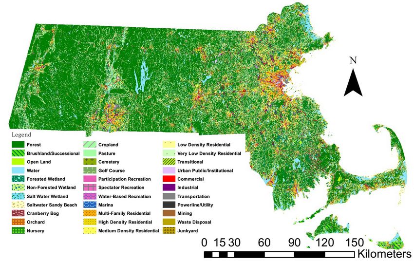
Int. J. Environ. Res. Public Health 2018, 15, 250                                                    2 of 15

understand the social dynamics in urban areas [7]. For example, Lansley and Longley [8] systematically
studied the geography of Twitter topics in London, and found topics expressed through tweets varied
significantly across different land uses and times in Inner London. The mobility patterns of Twitter
users can also be used to classify urban land use types with reasonable accuracy [9]. These studies
demonstrated the feasibility of tracking social trends across time and space with Twitter data.
      In addition to spatiotemporal information, the contents of tweets also provide substantial
information regarding users’ opinions and sentiment. Quantifiably interpreting tweets relies on
employing sentiment analysis [10], which is used to computationally translate opinions and expressions
of human sentiment into data that can be quantified and categorized [10]. Specifically, a major focus of
sentiment analysis tools is identifying the positive, neutral, or negative polarity of a given text [11].
Identification of the polarity by Twitter users has been used to study the geographical property of
public sentiment during Hurricane Sandy [12]. Extracting sentiments during disaster events can help
develop stronger situational awareness of the disaster zone. Jiang et al. [13] used sentiment analysis to
systematically assess the online public onions on an ex-post evaluation of a large infrastructure project
in China. Yu and Wang [14] performed sentiment analysis to examine U.S. soccer fan’s emotional
reactions towards the World Cup 2014 games from their tweets. They found strong relationships
between the fan’s sentiment, participated teams, and goal results. Palomino et al. [15] conducted
sentiment analysis for 175,000 tweets related to the natural-deficit disorder. They concluded that the
dissemination of nature-health concepts was associated with both the hashtags used and the sentiment
of the message. A recent study applying sentiment analysis of geo-tagged tweets about food revealed
the prevalence of healthy and unhealthy food across the continental USA [16]. Their findings can be
used to identify regions that have low access to healthy food.
      As exemplified in these research examples, Twitter data are increasingly perceived as “social
sensors” to better understand the social phenomenon in the real world [17]. Twitter data have already
been used to provide valuable information about public issues on myriad topics, e.g., outdoor air
pollution [18], opinion polling [19], stock markets [20], and elections [21]. There is also a growing
interest in Twitter-based approaches for public health research [22]. One important use of Twitter data
in health-related research is disease surveillance and prevention, such as influenza outbreaks [23] and
HIV prevalence [24]. These studies indicated that the epidemic spreading in the real world can be well
traced in relevant tweets. A recent review paper [25] proved that sentiment analysis of Twitter data has
been used in many different domains to solve various problems. The greatest value of this discipline is
to extract the intrinsic knowledge disseminated in tweets to help government or business intelligence.
      In addition, there has been an increasing number of studies that use Twitter data to measure and
analyze the quality of life (QoL) and happiness in cities and regions, aiming to find out what makes a
“happy city” [26]. QoL is a measure of social well-being and life satisfaction of people in cities/regions.
Most of the efforts are still based on objective measures of QoL, including income, housing, urban land
use, natural environment, environmental pollution, and local amenities, etc. These objective indicators
are relatively easy to be quantified for ranking the urban and regional QoL [27,28]. On the other
hand, increasing attention has also been paid to the evaluation of subjective QoL, such as subjective
happiness and well-being. Previous quantitative studies of happiness are normally based on subjective
measures of well-being derived by questionnaire surveys [29,30]. Oswald and Wu [31] explored the
life satisfaction in each state based on the results from U.S. Behavioral Risk Factor Surveillance System.
They confirmed a state-by-state match between subjective and objective well-being. Recent studies
already suggest that while most of the variations in subjective well-being are attributable to individual
characteristics, some of the variations can also be associated with the geographical context and regional
factors [32,33]. It is necessary to investigate the impact of geographical context upon subjective QoL.
Bhatti et al. [34] spatially examined the relationships between surveyed QoL, land use and population
density in an urban environment of Lahore. An inverse relationship was observed between QoL
with built-up and population densities. Some researchers also studied the geographical distributions
of subjective QoL in cities based on GIS approaches [35–37]. These studies proved that reasonable
Int. J. Environ. Res. Public Health 2018, 15, 250 3 of 15
planning of land use was an important factor for building a successful city with both high objective
and subjective QoL.
As introduced above, Twitter data provide a more economical and dynamic approach compared
to traditional population survey and, more importantly, an ability to add objective geometrical
dimension to the subjective study of QoL. It is being recognized that there is a great potential
in identifying key spatial characteristics and factors of cities and regions pertaining to subjective
well-being measures. The users’ sentiment expressed by tweets is likely to vary in different surrounding
environments and time periods, according to the user’s activities and opinions. Some studies have
been carried out combining sentiment analysis, spatiotemporal analysis, and domain knowledge
for public well-being. Yang and Mu [38] applied GIS methods to Twitter data to detect clusters of
major depressive disorder users. They provided an alternative way to diagnose depression in a
large population. Nguyen et al. [39] built up a neighborhood dataset of happiness, diet, and physical
activity across the 2010 census tracts of the U.S. based on a large corpus of tweets. They concluded
that the tracts with the social and economic disadvantage, high urbanization, and more fast food
restaurants may exhibit lower happiness and fewer healthy behaviors. Mitchell et al. [40] also studied
the geography of happiness across all 50 U.S. states based on a large dataset of tweets. Happiness
within each city/state was found to be positively correlated with wealth and anti-correlated with
obesity rates. Another group of researchers investigated the weekly trend of emotion and work stress
by Twitter analysis [41]. The linguistic inquiry word counts indicated a clear “Friday dip” for work
stress and negative emotion tweets and a “weekend peak” for positive emotion tweets.
Current studies mainly focused on the descriptive analyses of users’ polarity and mobility patterns.
However, less attention has been paid to the spatiotemporal patterns of users’ sentiment scores by
using statistical analyses. To address this issue, we emphasized both the land use/time aspects and the
quantified sentiment scores from Twitter data in this study. In this paper, we used Twitter data along
with high-resolution land use data to reveal the spatiotemporal variations of public sentiment, through
a corpus of nearly one million of georeferenced tweets collected within Massachusetts (MA), USA.
The MassGIS data were used to classify the land use categories. Computational sentiment analysis
was employed to quantitatively identify the users’ polarity with sentiment scores from the collected
tweets on a large scale. We further used a multivariate linear mixed-effects model to statistically reveal
the prevalence of users’ sentiment across different geographical locations and time periods. This case
study demonstrated an economical approach to investigate the spatiotemporal patterns of subjective
QoL of Twitter users in cities and regions.
2. Materials and Methods
2.1. Twitter Data
The study is based on a Twitter dataset of 880,937 tweets posted by 26,060 users within
Massachusetts, USA from 31 November 2012 to 3 June 2013, collected via the Twitter streaming
API (application program interface). Tweets were collected within a one-mile radius of all private and
public schools in Massachusetts (kindergarten to grade 12, n = 2613 [42]). The one-mile radius of these
schools can basically encompass all urban/suburban areas in Massachusetts. All the collected tweets
were restricted to those with precise geographical locations, post time, original content in English,
and active users posting more than 10 and less than 270 tweets (equivalently up to 1–2 tweets/day)
within the timeframe. This restriction aimed to avoid non-active users with fewer than ten posts and
hyperactive users that often belong to commercial entities or twitter bots. We restricted the criteria to
geo-tagged tweets to gain the geolocation of the sampled tweets as accurate as the mobile phone’s
location, which is accurate to about a range of 8 m [43].
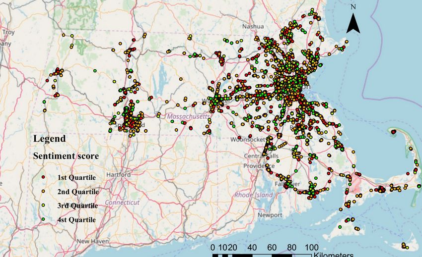
The geotagged tweets were mapped out with the land use data by using the ArcGIS Desktop
10.4.1 (Esri, Redlands, CA, USA). Then the land use types were correspondingly attributed to those
tweets which fell within their polygons based on the geographical coordinates. Figure 1 shows the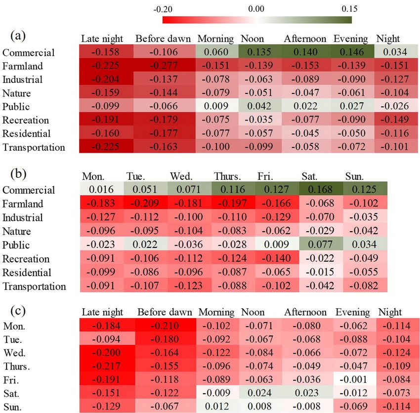
Int. J. Environ. Res. Public Health 2018, 15, x 4 of 16
created using semi-automated methods, and based on the 0.5-m resolution digital orthoimagery
captured in April 2005. The minimum mapping unit (MMU) is generally one acre, but an MMU
Int. J. Environ. Res. Public Health 2018, 15, 250
as
4 of 15
low as 0.25 acre may be found in some urban areas. A more detailed definition of each land use type
can be found on the MassGIS website [44]. The land use types were further grouped into eight
geographical
categories distribution
according of 33 intra-similarities,
to their land use types in MA, mapping
as shown in based
Tableon1.the
TheMassGIS landnursery
cemetery, use dataand
[44].
The data layer contains a Massachusetts statewide, seamless digital dataset
transitional land uses were excluded from analysis due to their limited sample sizes. The land of MAof land cover/land use,
created
was using
largely semi-automated
covered by the land methods,
use category andofbased
nature,onfollowed
the 0.5-mbyresolution digital
the residential andorthoimagery
commercial
captured
land in April
uses that 2005. Theconcentrated
are typically minimum mapping unit (MMU) is generally
in the urban/suburban areas. Theone acre, but
collected an MMU
number as low
of tweets
as 0.25 acre may be found in some urban areas. A more detailed
(Table 1) was correspondingly related to the coverage of each land use category. definition of each land use type can
be found on the MassGIS
The temporal website
information [44].tweets
of the The landwasusealsotypes were further
classified for the grouped
statisticalinto eight categories
analysis. The time
according
periods of toa their intra-similarities,
day were classified into:as shown in Table
late night 1. The cemetery,
(00:00–3:00), before nursery and transitional
dawn (3:00–6:00), land
morning
uses were excluded
(6:00–11:00), from analysis due
noon (11:00–13:00), to their(13:00–18:00),
afternoon limited sampleevening
sizes. The land of MA and
(18:00–21:00), was largely
night
covered by theThe
(21:00–00:00). land use category
percentages of of nature,
the tweets followed
collected byduring
the residential andperiods
these time commercialwereland uses
3.5%, that
3.5%,
are typically
20.7%, 10.6%,concentrated
28.0%, 20.7%, in the
and urban/suburban
13.0%, respectively.areas. The collected
days of number
the week of tweets (Table 1)into
were divided was
correspondingly
weekdays (Mon., related to theThurs.
Tue., Wed., coverage
and of each
Fri.), land
and use category.
weekend (Sat. and Sun.).
Figure
Figure1.1.Geographical
Geographicaldistribution
distributionof
of33
33land
landuse
usetypes
typeswithin
withinMA
MA(mapping
(mappingbased
basedon
onthe
theMassGIS
MassGIS
land
landuse
usedata
data[44]).
[44]).
Table
Table1.1.Classification
Classificationof
ofland
landuse
usein
inMA.
MA.
Number of
Category
Category LandUse
Land UseType
Type Number of Tweets
Tweets
Commercial
Commercial Commercial
Commercial 35,610
35,610
Farmland
Farmland CranberryBog,
Cranberry Bog,Cropland,
Cropland,Orchard,
Orchard,Pasture
Pasture 14,951
14,951
Industrial Industrial, Junkyard, Mining, Powerline/Utility, Waste Disposal 14,292
Industrial Industrial, Junkyard, Mining, Powerline/Utility, Waste Disposal 14,292
Brushland, Forest, Forested Wetland, Non-Forested Wetland, Open Land,
Nature Brushland, Forest, Forested Wetland, Non-Forested Wetland, Open Land, 567,086
Nature Saltwater, Sandy Beach, Saltwater Wetland, Water 567,086
Saltwater, Sandy Beach, Saltwater Wetland, Water
Public Urban Public/Institutional 27,786
Public Urban Public/Institutional
Golf Course, Marina, Participation Recreation, Spectator Recreation, Water-based 27,786
Recreation 21,365
Recreation
Golf Course, Marina, Participation Recreation, Spectator Recreation,
Recreation 21,365
High Density Residential, Low Density Residential,
Water-based Recreation Medium Density Residential,
Residential 181,577
Multi-Family Residential, Very Low Density Residential
High Density Residential, Low Density Residential, Medium Density Residential,
Residential
Transportation Transportation 181,577
17,981
Multi-Family Residential, Very Low Density Residential
Excluded Cemetery, Nursery, Transitional 289
Transportation Transportation 17,981
Excluded Cemetery, Nursery, Transitional 289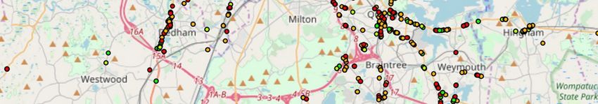
Int. J. Environ. Res. Public Health 2018, 15, 250                                                                            5 of 15

     The temporal information of the tweets was also classified for the statistical analysis. The time
periods of a day were classified into: late night (00:00–3:00), before dawn (3:00–6:00), morning
(6:00–11:00), noon (11:00–13:00), afternoon (13:00–18:00), evening (18:00–21:00), and night (21:00–00:00).
The percentages of the tweets collected during these time periods were 3.5%, 3.5%, 20.7%, 10.6%, 28.0%,
20.7%, and 13.0%, respectively. The days of the week were divided into weekdays (Mon., Tue., Wed.,
Thurs. and Fri.), and weekend (Sat. and Sun.).

2.2. Data Analysis
     We used the IBM Watson Alchemy application program interface (API) [45] to conduct sentiment
analysis of the collected tweets, which has been trained on billions of web pages and can provide
cloud-based natural language processing. The Alchemy API introduces a combined use of linguistic
analysis, which considers a sentence’s composition, and statistical analysis, which handles noisy
content. Its sentiment analysis is built upon machine-learned patterns to predict the intended sentiment
from text. The Alchemy API has been verified as one of the best sentiment classification tools, especially
for tweets [46]. Alchemy API’s sentiment analysis could reach an accuracy of 88.36% and 86% for
2100 hotel reviews from TripAdvisor [47], and a corpus of 5370 tweets on tourism [48], respectively.
The calculated sentiment score has a continuous value range of [−1, 1], referring to the polarity from
extremely negative to extremely positive. Zero means the sentiment is neutral.
     Bar charts were used to graphically depict the distributions of average sentiment scores per
different influencing factors. We also used the net sentiment rate (NSR) to judge the overall attitudes
expressed by users through comparing the rate of positive and negative tweets (Equation (1)).
The prevalence of users’ sentiment could be clearly revealed by looking at both the score distributions
and the NSR:
                                         Positive Tweets − Negative Tweets
                               NSR =                                                                   (1)
                                               Total number o f Tweets
     Heat maps were used to present the mobility pattern of users, by using the open-source statistical
package R version 3.4.0 (R Project for Statistical Computing, Vienna, Austria). The “plyr” package was
used to count the number of users across land use categories and time periods. The heat maps were
plotted out by using the “ggplot2” package, and further polished by using the “ggthemes”, “scales”
and “viridis” packages.
     In addition to the descriptive analysis, a multivariate linear mixed-effects model was used to
quantify the effects of land use and time period on the sentiment score of the individual user. Analyses
were performed by using the “nlme” package in R. The regression model is:

  yi,j,k,l = β 0 + β 1 ∗ L1 + · · · + β 7 ∗ L7 + β 8 ∗ D1 + · · · + β 13 ∗ D6 + β 14 ∗ T1 + · · · + β 19 ∗ T6 + b0,i + ε i,j,k,l (2)

where yi,j,k,l is the sentiment score for user i in land use category j during time period l on day k. We fitted
the model with a random effect b0,i of the intercept for user i to account for the clustering effect of each
individual user, and we included a categorical variable of land use category (Lj ), a categorical variable
of the days of the week (Dk ) and a categorical variable of the time periods of the day (Tl ) as the fixed
effects in the model. β0 is the fixed intercept; β1 –β7 are the fixed effects of other land use categories
compared to farmland; β8 –β13 are the fixed effects of other days of the week compared to Wednesday;
β14 –β19 are the fixed effects of other time periods of the day compared to before dawn; and ε i,j,k,l is the
vector of random errors.

3. Results
     Figure 2 displays the geographical distributions of the collected tweets with quartiles of sentiment
scores. Most of the tweets were posted within urban/sub-urban centers, such as the Greater Boston
Area, Springfield, Worcester, and Pittsfield. Seventy-eight percent of the collected tweets expressed
either positive (36%) or negative (42%) attitudes from users, while the other 22% of tweets conveyed
Int. J. Environ. Res. Public Health 2018, 15, 250                                                                    6 of 15

neutral sentiment. On average, the users’ sentiment conveyed by these tweets tended to be skewed to
slightly negative with an average score of −0.053 and an NSR of −0.065.
    Int. J. Environ. Res. Public Health 2018, 15, x                                                              6 of 16

                                                           (a)

                                                           (b)
          Figure
      Figure      2. Geographical
              2. Geographical       distributionof
                                 distribution    oftweets
                                                    tweets with
                                                           with quartiles
                                                                 quartilesofofsentiment
                                                                               sentimentscores in in
                                                                                          scores  (a)(a)
                                                                                                      Massachusetts
                                                                                                         Massachusetts
          and (b) Greater Boston area. First quartile (−1.000 to −0.410), second quartile (−0.410 to 0.000), third
      and (b) Greater Boston area. First quartile (−1.000 to −0.410), second quartile (−0.410 to 0.000),
          quartile (0.000 to 0.514), and fourth quartile (0.514 to 1.000).
      third quartile (0.000 to 0.514), and fourth quartile (0.514 to 1.000).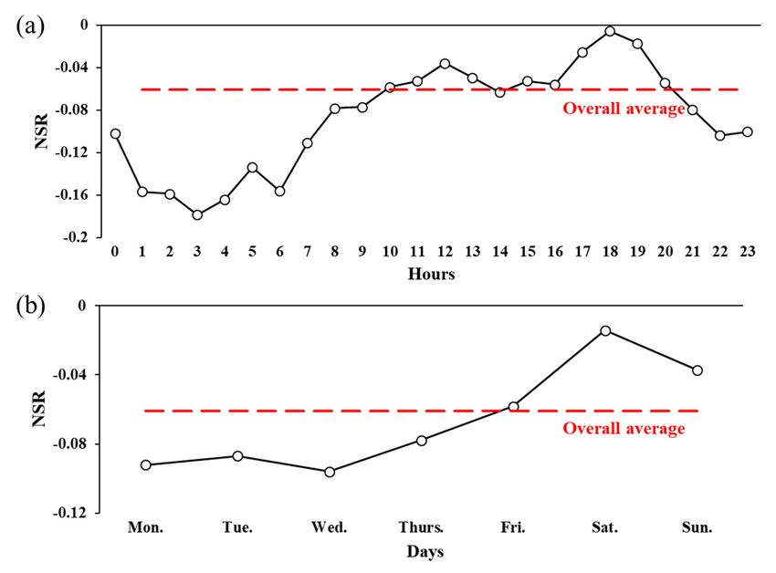
Int. J. Environ. Res. Public Health 2018, 15, 250 7 of 15
Int.
Int.J.J.Environ.
Environ.Res.
Res.Public
PublicHealth
Health2018,
2018,15,
15,xx 77of
of16
16
Figure 3 shows the distribution of average sentiment scores across the eight land use categories.
Figure
Figure33 showsshows the thedistribution
distribution of ofaverage
average sentiment
sentimentscores
scores across
acrossthe the eight
eightlandlanduseuse categories.
categories.
Commercial land use was the only area where sentiment scores were skewed to be positive, with 37%
Commercial
Commercialland landuseusewaswasthe
theonly
onlyarea
areawhere
wheresentiment
sentimentscores
scoreswerewereskewed
skewedto tobebepositive,
positive,withwith37% 37%
more positive tweets than negative tweets. The lowest average sentiment score was found in the area
more
morepositive
positivetweetstweetsthanthannegative
negativetweets.
tweets.TheThelowest
lowestaverage
averagesentiment
sentimentscore scorewaswasfound
foundin inthe
thearea
area
of farmland, with nearly 50% more negative tweets compared to positive tweets. Another interesting
of
offarmland,
farmland,with withnearly
nearly50% 50%more
morenegative
negativetweets
tweetscompared
comparedto topositive
positivetweets.
tweets.Another
Anotherinteresting
interesting
finding
finding was that the positive and negative scores were almost evenly distributed in the public area.
finding was was that
that the
the positive
positive and
and negative
negative scores
scores were
were almost
almost evenly
evenly distributed
distributed in in the
the public
public area.
area.
AsAs
Asshown
showninin
shown inFigure
Figure4,
Figure 4,the
4, thevariation
the variation trend
variation trend
trend ofofnormalized
of normalizedpolarity
normalized polarity
polarity waswas
was highly
highly
highly relevant
relevant
relevant to to
thethe
to the trendtrend
trend of of
of
average
average sentiment
average sentiment scores
sentiment scores by
scores by land
by land use
land use categories.
use categories. The
categories. The commercial
The commercial
commercial area area
area was was mainly
was mainly concentrated
mainly concentrated
concentrated in in in
urban
urban
urban regions,
regions,where
regions, whereusers
where usersshowed
users showed
showedmore more positiveemotions
morepositive
positive emotionswith
emotions with
with anan
an average
average
average sentiment
sentiment
sentiment score
score
score of of 0.047
of0.047
0.047
and
and a aNSR
NSR of
of 0.099.
0.099. The
The overall
overall polarity
polarity tended
tended to
to be
be neutral
neutral in in
thethe public
public
and a NSR of 0.099. The overall polarity tended to be neutral in the public area with a NSR of 0.010. areaarea
withwith
a a
NSR NSRof of
0.010.0.010.
The
The average
The average sentiment
average sentiment scores
sentiment scores were
scores were approximately
were approximately around
approximately around
around the the overall
the overall average
overall average
average score score ( −
score (−0.053) 0.053)
(−0.053) in thethe
in
in the
areas
areas
areas ofof
ofresidence,
residence,nature,
residence, nature,and
nature, andrecreation.
and recreation. Userswere
recreation. Users
Users weremore
were morelikely
more likelyto
likely toto show
show
show negative
negative
negative emotions
emotions
emotions within
within
within
the
the
theareas
areasofof
areas oftransportation,
transportation,industry,
transportation, industry, andand farmland.
and farmland.
farmland. TheThespatial
The spatialvariations
spatial variations
variations ofof
of the
thethe average
average
average sentiment
sentiment
sentiment
scores
scores
scores indicated
indicated
indicatedthat that users’
thatusers’ emotions
emotions could
users’emotions could probably
could probably be
probably beaffected
be affectedby
affected bythe
by thesurrounding
the surrounding
surrounding environments.
environments.
environments.
Figure
Figure3. Averagesentiment
3.Average sentimentscores
sentiment scoresby
scores byland
by land
land use
use
use categories.
categories.
categories.
Figure
Figure NSRs
Figure4.4.NSRs by land
NSRsby landuse
usecategories.
use categories. NSR:
categories.NSR:
NSR: net
net
net sentiment
sentiment
sentiment rate.
rate.
rate.
The
The sentiment
Thesentiment scores
sentimentscores showed
showed clear
scoresshowed clear temporal
clear temporalpatterns
temporal patternsby
patterns bybyhours
hours
hours of the
ofofthe day
theday and
dayand days
days
and of
of the
days the week,
week,
of the week,
as
as shown
shown in
in Figures
Figures 55 and
and 6.
6. ItIt is
is clear
clear that
that users’
users’ sentiment
sentiment followed
followed aa certain
certain temporal
temporal pattern
pattern
as shown in Figures 5 and 6. It is clear that users’ sentiment followed a certain temporal pattern
throughout
throughoutthe theday.
day.From
Fromlate
latenight
nightto toearly
earlymorning,
morning,the theaverage
averagesentiment
sentimentscores
scoreswere
weremuch
muchlower
lower
throughout the day. From late night to early morning, the average sentiment scores were much lower
than
than the
the overall
overall mean
mean score,
score, reaching
reaching the the lowest
lowest at
at 3:00
3:00 with
with aa value
value ofof−0.119
−0.119 and
and an
an NSR
NSR of of −0.179.
−0.179.
than the overall mean score, reaching the lowest at 3:00 with a value of −0.119 and an NSR of −0.179.
The
The sentiment
sentiment scores
scores began
began toto increase
increase fromfrom noon
noon and
and showed
showed two two peaks
peaks during
during 11:00
11:00 to
to 13:00
13:00 and
and
The sentiment scores began to increase from noon and showed two peaks during 11:00 to 13:00 and
17:00
17:00 toto 20:00.
20:00. The
The average
average sentiment
sentiment scoresscores during
during 10:00
10:00 to
to 20:00
20:00 were
were higher
higher than
than the
the overall
overall mean
mean
17:00
score.
to 20:00. The average sentiment scores during 10:00 to 20:00 were higher than the overall mean
score.TheTheaverage
averageusers’
users’sentiment
sentimentwas wasobviously
obviouslylifted
liftedononthe
theweekend,
weekend,with withaamean
meanscore
scoreof of−0.030
−0.030
score.
and
and an
The
an NSR
average
NSR of
users’
of −0.026.
−0.026. The
sentiment
The average
was
average sentiment
obviously
sentiment score
lifted on
score decreased
the
decreased to
weekend,
to −0.063
−0.063 on
with a mean
on weekdays,
weekdays, along
score
along with
of −
with an
0.030
an
and an NSR of −0.026. The average sentiment score decreased to −0.063 on weekdays, along with an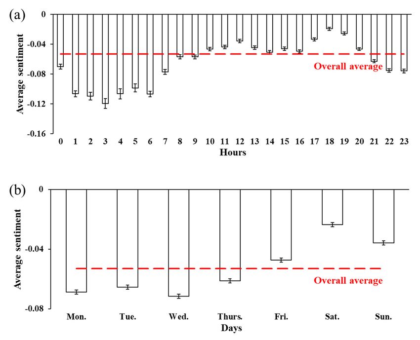
highest was on Friday, with a value of −0.047 and an NSR of −0.058.
        The temporal patterns of users’ sentiment could be partially explained by the daily routine of
the general public. During the day, the two peaks of sentiment scores were during 11:00 to 13:00 and
17:00 to 20:00, which were the typical time periods for relaxation, dining, or hanging out. The most
negative sentiment appeared around 3:00 when users possibly felt more emotional or anxious
Int. J. Environ. Res. Public Health 2018, 15, 250                                                             8 of 15
because of staying up around midnight. Users also tended to be unhappy when getting up early in
the morning. The weekly trend shows a clear “mid-week dip” and a “weekend peak” for users’
sentiment,
NSR of −0.082.  quiteTheconsistent
                             averagewith    the findings
                                       sentiment   scoresby another
                                                          were       Twitter-based
                                                               generally  lower thanlinguistic inquiry
                                                                                       the overall       study
                                                                                                   average     [41].
                                                                                                             among
This    can bereaching
weekdays,        interpreted     as the on
                            the lowest    weekend’s   recovery
                                              Wednesday  with aeffects on−working
                                                                value of   0.072 andpressure,
                                                                                      an NSR ofas −
                                                                                                  indicated  by the
                                                                                                    0.096, while the
lifted   sentiment     score  on   Friday.
highest was on Friday, with a value of −0.047 and an NSR of −0.058.

Int. J. Environ. Res. Public
                 Figure
                  Figure   5.Health
                          5. Average2018,
                              Average     15, x
                                       sentiment scores by (a) hours of the day and (b) days of the week.     9 of 16

                         Figure 6. NSRs
                                   NSRs by (a) hours of the day and (b) days of the week.

     Figure 7 showspatterns
     The temporal    the spatiotemporal  variations
                             of users’ sentiment     in the
                                                  could  be users’ sentiment.
                                                            partially         Figure
                                                                      explained      7a,b
                                                                                 by the   show
                                                                                        daily   that the
                                                                                              routine of
NSRs  varied greatly by different time periods in each land  use category. The variation trends of NSRs
the general public. During the day, the two peaks of sentiment scores were during 11:00 to 13:00 and
were consistent with the temporal patterns shown in Figure 6. The overall sentiment was higher from
noon to evening, and lower during midnight to early morning, the same as in all of the land use
categories. The NSRs were also obviously higher on the weekend compared to weekdays in all the
land use categories. From another perspective, the NSRs also varied by different land use categories
during each time period. The variations of NSRs by land use were also consistent across all the time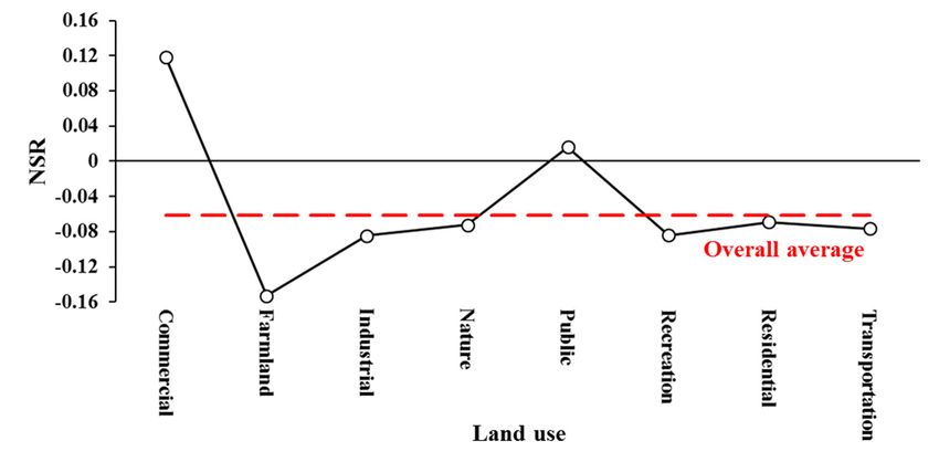
Int. J. Environ. Res. Public Health 2018, 15, 250                                                           9 of 15

17:00 to 20:00, which were the typical time periods for relaxation, dining, or hanging out. The most
 negative sentiment appeared around 3:00 when users possibly felt more emotional or anxious because
 of staying up around midnight. Users also tended to be unhappy when getting up early in the
 morning. The weekly trend shows a clear “mid-week dip” and a “weekend peak” for users’ sentiment,
quite consistent with the findings by another Twitter-based linguistic inquiry study [41]. This can be
 interpreted as the weekend’s recovery effects on working pressure, as indicated by the lifted sentiment
 score on Friday.
        Figure 7 shows the spatiotemporal variations in the users’ sentiment. Figure 7a,b show that the
 NSRs varied greatly by different time periods in each land use category. The variation trends of NSRs
were consistent with the temporal patterns shown in Figure 6. The overall sentiment was higher from
 noon to evening, and lower during midnight to early morning, the same as in all of the land use
 categories. The NSRs were also obviously higher on the weekend compared to weekdays in all the
 land use categories. From another perspective, the NSRs also varied by different land use categories
 during each time period. The variations of NSRs by land use were also consistent across all the time
periods, following the trend in Figure 5. As shown in Figure 7c, the NSR reached a peak during the
 evening and went down to a bottom during the midnight every day throughout a week. The effects of
 land
Int.     use and
     J. Environ. Res.time  period
                       Public        were15,likely
                              Health 2018,    x    to be additive of the users’ sentiment.        10 of 16

      Figure 7. NSRs by (a) land uses and times of the day; (b) land uses and days of the week; and (c) times
      Figure 7. NSRs by (a) land uses and times of the day; (b) land uses and days of the week; and (c) times
      of the day and days of the week.
      of the day and days of the week.

     Except for the descriptive analysis, we used a multivariate linear mixed-effects model to quantify
the influence of land use and time period on the sentiment scores, accounting for the clustering effect
of users. The coefficients of each fixed variable shown in Table 2 were already modified by the
random effects of users and other fixed effects. The category with the lowest average sentiment score
was selected as the referent for each categorical variable. Therefore, these coefficients indicated the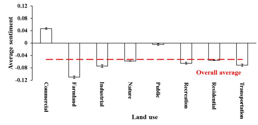
Int. J. Environ. Res. Public Health 2018, 15, 250                                                         10 of 15

     Except for the descriptive analysis, we used a multivariate linear mixed-effects model to quantify
the influence of land use and time period on the sentiment scores, accounting for the clustering effect
of users. The coefficients of each fixed variable shown in Table 2 were already modified by the random
effects of users and other fixed effects. The category with the lowest average sentiment score was
selected as the referent for each categorical variable. Therefore, these coefficients indicated the relative
effect intensities of different variables. The interaction between variables could be neglected due to
their very low cross-correlation coefficients. The model results were generally consistent with the
descriptive analysis above. The results clearly show the significant intra-category differences in the
average sentiment score for all the categorical variables. The average sentiment scores were obviously
higher in the commercial and public areas, during the weekends, and between noon and evening,
compared to their respective references. The regression model was also used to compare the users’
sentiment in certain land use category and time period. For example, the average sentiment score was
increased by a value of 0.148 (p < 0.0001) in the commercial area during Saturday evening, compared
to the score on farmland before dawn on Wednesday.

                             Table 2. Summary of fixed effect estimates on sentiment scores.

                    Variables                       Coefficients of Fixed Effects   Standard Error   p-Value
                    Intercept                                  −0.111                   0.007
Int. J. Environ. Res. Public Health 2018, 15, 250 11 of 15
formulate appropriate public policies or marketing methods in different cities and regions. On the
other hand, it can also be used for evaluating the implementation of measures for improving the
subjective QoL.
Figure 8 shows the mobility patterns of users by land use categories. In general, the two peaks of
user activity were observed during the lunchtime and the evening hours, similar to the findings of a
previous study [9]. Twitter users were most active from 18:00 to 21:00 (27% of the tweets were posted),
especially in the commercial area. It is also shown that users were more active during the weekend
compared to the weekdays. Nevertheless, the number of active users was obviously lower in the early
morning on the weekend. Different land use categories also manifested distinctive patterns. In the
commercial and public areas, users were obviously more active in the daytime during the weekend
than weekdays. In the areas of nature and residence, users showed regular activity patterns. The land
use category of nature does not necessarily mean remote areas. In contrast, a large portion of natural
land use types are located in the suburban areas near green land or water, where a large number of
local residents live. This could be the reason for the similar patterns of users’ sentiment and activity in
the natural and residential areas. For the other land use categories, the temporal frequency of users
Int. J. Environ.
generally Res. Publicthe
followed Health 2018, 15,
overall x
trend, but showed more irregular patterns. 12 of 16
Figure
Figure 8.
8. Temporal
Temporal frequency
frequency of active users
of active users by
by land
land use
use categories.
categories.
The date or seasonal pattern of sentiment is not explicitly discussed in this paper, because it is
The date or seasonal pattern of sentiment is not explicitly discussed in this paper, because it is
more likely to be associated with social events, public holidays, and climate environments. Figure 9
more likely to be associated with social events, public holidays, and climate environments. Figure 9
shows the variations of sentiment over the investigated date range. As shown in the figure, the users’
shows the variations of sentiment over the investigated date range. As shown in the figure, the users’
sentiment was very sensitive to the date when it is collected. It is clear that extreme NSR values were
sentiment was very sensitive to the date when it is collected. It is clear that extreme NSR values were
highly correlated with important social events, extreme weather, and public holidays. For instance,
highly correlated with important social events, extreme weather, and public holidays. For instance,
users showed obviously more positive sentiment on Christmas, New Year, Valentine’s Day, Easter,
users showed obviously more positive sentiment on Christmas, New Year, Valentine’s Day, Easter,
and Mother’s Day, etc. The extremely negative sentiment was likely to be caused by bad weather or
and Mother’s Day, etc. The extremely negative sentiment was likely to be caused by bad weather or
certain social events, e.g., the Boston Marathon Bombings. After the bombings, the average sentiment
certain social events, e.g., the Boston Marathon Bombings. After the bombings, the average sentiment
score soon returned to a peak value when the second suspect was arrested on 20 April 2013.
score soon returned to a peak value when the second suspect was arrested on 20 April 2013.sentiment was very sensitive to the date when it is collected. It is clear that extreme NSR values were
highly correlated with important social events, extreme weather, and public holidays. For instance,
users showed obviously more positive sentiment on Christmas, New Year, Valentine’s Day, Easter,
and Mother’s Day, etc. The extremely negative sentiment was likely to be caused by bad weather or
certain social events, e.g., the Boston Marathon Bombings. After the bombings, the average sentiment
Int. J. Environ. Res. Public Health 2018, 15, 250 12 of 15
score soon returned to a peak value when the second suspect was arrested on 20 April 2013.
Figure
Figure9.9.Variations
Variationsof
ofNSRs
NSRsduring
duringthe
theinvestigated
investigateddate
daterange.
range.
There are several limitations to this research. We used the main categories of land use due to the
insufficient sample size of tweets in many sub-group types. The underlying variations of sentiment
across nuanced land use types may be overlooked if just studying the eight main categories. Moreover,
the intensively urban/suburban usage (Figure 2) indicates that our results are more representative of
the population in non-rural regions. A larger and more widely-distributed set of tweets is necessary
to study the influence of land use types on public sentiment at a finer spatial scale. The mobility of
Twitter users is also a confounder of our analysis. It could be possible that the users’ sentiment were
less relevant to the posting location due to their mobility. However, using a big data approach and
treating the user as a random effect in linear modeling may help reduce this kind of confounding effect.
The interpretation of Twitter-based results also needs to be cautious. Opinions conveyed by users
are strongly influenced by their characteristics. Twitter is a means of spreading information publicly,
thus, the information and the nature of how it is expressed vary among users. Most of the variations
in subjective well-being are still attributable to individual characteristics [32,33]. We considered the
clustering effect of users in our modeling analysis, but that only represented a small part of users’
characteristics. The marginal R-squared value of fixed effects is 0.7% and the conditional R-squared
value of the model is 10.4% for both the fixed and random effects. Therefore, the proposed model
was not applicable for prediction. Instead, the model was mainly used to find out the intra-category
differences in average sentiment scores.
The demographic and social-economic characteristics of individual users are also strongly
associated with the variations in what is communicated through Twitter [2]. A case study in
Chicago [49] indicates that the demographic information, particular the race/ethnicity group,
significantly affects the urban mobility patterns of Twitter users. As Twitter does not require users to
record detailed personal information, it is not possible to obtain personal characteristics conclusively.
A recent study showed that the age and gender characteristics could be inferred from 32,000 unique
forenames representing over 17 million individuals in Britain [50]. This kind of approach may not
cover all the Twitter users because a large portion of users prefer to use nicknames instead of full
names. Demographic and neighborhood socio-economic characteristics of users can be approximately
assigned according to the social census statistics [16]. However, the assigned characteristics may be
biased due to the strong mobility of users. Further studies are needed to address the relationships
between these individual differences and the spatiotemporal variations in users’ sentiment. In addition,
the use of the Twitter service is selective. This leads to a major limitation of Twitter-based analysis that
the sampled population may not be completely representative of the population of interest. TwitterInt. J. Environ. Res. Public Health 2018, 15, 250 13 of 15
users only account for 15% of Internet-using adults, mostly including young adults, African Americans,
urban/suburban residents, and mobile users [51]. Moreover, only the geo-tagged tweets that users
would like to share publicly can be used for this type of study, which implicates bias from the selective
disclosure of information and location. Therefore, it should be noticed that the Twitter-based research
results are unable to represent the total population in the studied region.
Finally, a tweet is challenging to be classified as the content is restricted to 140 characters,
while usually including nuanced or ambiguous words. Some users may even convey opinions with
bi-polarity. We manually verified the Alchemy API using 500 randomly-selected tweets (170 positive,
160 neutral, and 170 negative) from our Twitter dataset, and the overall accuracy can reach 80.6%.
The identification accuracy for positive, neutral, and negative tweets were 82.9%, 87.3%, and 72.1%,
respectively. The Alchemy API works very well in the identification of neutral polarity, but sometimes
confuses the negative and positive opinions. Using a large sample size of tweets may help reduce
the uncertainties in the average sentiment scores. Moreover, the complex emotional state of human
may not be completely expressed using a one-dimensional sentiment scale. Human emotions can be
further classified into eight types: anger, fear, joy, sadness, disgust, surprise, trust, and anticipation [52].
Further studies are recommended to analyze these emotions conveyed from tweets to gain a deeper
insight of public sentiment.
5. Conclusions
This study clearly revealed the spatiotemporal variations of users’ sentiment within MA, based on
nearly one million randomly-collected tweets during a half year. The users’ sentiment was significantly
higher in the commercial and public areas, during the noon/evening and on the weekend. In contrast,
users were more likely to show negative sentiment within the areas of farmland, transportation, and
industry, around midnight and on weekdays. The multivariate linear mixed-effects model showed
that the average sentiment score could be increased by a value of 0.148 in the commercial area during
Saturday evening, compared to the score on farmland before dawn on Wednesday. The results are not
conclusive due to an insufficient sample size, lack of user information and generalized classification of
land use. However, the demonstrated approach can be further used to investigate public happiness
and well-being in cities and regions with more comprehensive datasets.
Acknowledgments: We thank the anonymous peer reviewers for their excellent comments that have enhanced
the manuscript. This research was unfunded and completed out of the academic interest of the authors.
Piers MacNaughton’s time was supported by NIEHS environmental epidemiology training grant 5T32ES007069-35.
Jie Yin’s funding is provided by the Harvard Campus Sustainability Innovation Fund. Joseph G. Allen’s funding
comes from his faculty startup funds.
Author Contributions: Xiaodong Cao, Piers MacNaughton, and Zhengyi Deng contributed to the methodological
approach, data analyses, and drafting of the manuscript. Jie Yin and Xi Zhang helped to draft the manuscript.
The research idea was inspired by Joseph G. Allen. He participated in the interpretation of the data and drafting
of the manuscript. All authors contributed to, read, and approved the final manuscript.
Conflicts of Interest: The authors declare no conflict of interest.
References
1. Twitter. Twitter Usage/Company Facts (Updated 30 June 2016). Available online: https://about.twitter.
com/company (accessed on 5 January 2017).
2. Li, L.; Goodchild, M.F.; Xu, B. Spatial, temporal, and socioeconomic patterns in the use of Twitter and flickr.
Cartogr. Geogr. Inf. Sci. 2013, 40, 61–77. [CrossRef]
3. Xu, C.; Wong, D.W.; Yang, C. Evaluating the “geographical awareness” of individuals: An exploratory
analysis of Twitter data. Cartogr. Geogr. Inf. Sci. 2013, 40, 103–115. [CrossRef]
4. Zhao, D.; Rosson, M.B. How and why people Twitter: The role that micro-blogging plays in informal
communication at work. In Proceedings of the ACM 2009 International Conference on Supporting Group
Work, Sanibel Island, FL, USA, 10–13 May 2009; pp. 243–252.Int. J. Environ. Res. Public Health 2018, 15, 250 14 of 15
5. Singleton, A.D.; Longley, P. The internal structure of greater london: A comparison of national and regional
geodemographic models. Geo: Geogr. Environ. 2015, 2, 69–87. [CrossRef]
6. Blei, D.M. Probabilistic topic models. Commun. ACM 2012, 55, 77–84. [CrossRef]
7. Longley, P.A.; Adnan, M.; Lansley, G. The geotemporal demographics of Twitter usage. Environ. Plan. A
2015, 47, 465–484. [CrossRef]
8. Lansley, G.; Longley, P.A. The geography of Twitter topics in london. Comput. Environ. Urban Syst. 2016, 58,
85–96. [CrossRef]
9. Soliman, A.; Soltani, K.; Yin, J.; Padmanabhan, A.; Wang, S. Social sensing of urban land use based on
analysis of Twitter users’ mobility patterns. PLoS ONE 2017, 12, e0181657. [CrossRef] [PubMed]
10. Balahur, A.; Mihalcea, R.; Montoyo, A. Computational approaches to subjectivity and sentiment analysis:
Present and envisaged methods and applications. Comput. Speech Lang. 2014, 28, 1–6. [CrossRef]
11. Abbasi, A.; Hassan, A.; Dhar, M. Benchmarking Twitter Sentiment Analysis Tools. In Proceedings of the
LREC, Reykjavik, Iceland, 26–31 May 2014; pp. 823–829.
12. Neppalli, V.K.; Caragea, C.; Squicciarini, A.; Tapia, A.; Stehle, S. Sentiment analysis during hurricane sandy
in emergency response. Int. J. Disaster Risk Reduct. 2017, 21, 213–222. [CrossRef]
13. Jiang, H.; Qiang, M.; Lin, P. Assessment of online public opinions on large infrastructure projects: A case
study of the three gorges project in China. Environ. Impact Assess. Rev. 2016, 61, 38–51. [CrossRef]
14. Yu, Y.; Wang, X. World cup 2014 in the Twitter world: A big data analysis of sentiments in US sports fans’
tweets. Comput. Hum. Behav. 2015, 48, 392–400. [CrossRef]
15. Palomino, M.; Taylor, T.; Göker, A.; Isaacs, J.; Warber, S. The online dissemination of nature–health concepts:
Lessons from sentiment analysis of social media relating to “nature-deficit disorder”. Int. J. Environ. Res.
Public Health 2016, 13, 142. [CrossRef] [PubMed]
16. Widener, M.J.; Li, W. Using geolocated Twitter data to monitor the prevalence of healthy and unhealthy food
references across the US. Appl. Geogr. 2014, 54, 189–197. [CrossRef]
17. Naaman, M.; Becker, H.; Gravano, L. Hip and trendy: Characterizing emerging trends on Twitter. J. Assoc.
Inf. Sci. Technol. 2011, 62, 902–918. [CrossRef]
18. Jiang, W.; Wang, Y.; Tsou, M.-H.; Fu, X. Using social media to detect outdoor air pollution and monitor air
quality index (AQI): A geo-targeted spatiotemporal analysis framework with Sina Weibo (Chinese Twitter).
PLoS ONE 2015, 10, e0141185. [CrossRef] [PubMed]
19. Woo, H.; Cho, Y.; Shim, E.; Lee, K.; Song, G. Public trauma after the sewol ferry disaster: The role of social
media in understanding the public mood. Int. J. Environ. Res. Public Health 2015, 12, 10974–10983. [CrossRef]
[PubMed]
20. Bollen, J.; Mao, H.; Zeng, X. Twitter mood predicts the stock market. J. Comput. Sci. 2011, 2, 1–8. [CrossRef]
21. Tumasjan, A.; Sprenger, T.O.; Sandner, P.G.; Welpe, I.M. Election forecasts with Twitter: How 140 characters
reflect the political landscape. Soc. Sci. Comput. Rev. 2011, 29, 402–418. [CrossRef]
22. Finfgeld-Connett, D. Twitter and health science research. West. J. Nurs. Res. 2015, 37, 1269–1283. [CrossRef]
[PubMed]
23. Broniatowski, D.A.; Paul, M.J.; Dredze, M. National and local influenza surveillance through Twitter:
An analysis of the 2012–2013 influenza epidemic. PLoS ONE 2013, 8, e83672. [CrossRef] [PubMed]
24. Stoové, M.A.; Pedrana, A.E. Making the most of a brave new world: Opportunities and considerations for
using Twitter as a public health monitoring tool. Prev. Med. 2014, 63, 109–111. [CrossRef] [PubMed]
25. Martínez-Cámara, E.; Martín-Valdivia, M.T.; Urena-López, L.A.; Montejo-Ráez, A.R. Sentiment analysis in
Twitter. Nat. Lang. Eng. 2014, 20, 1–28. [CrossRef]
26. Ballas, D. What makes a ‘happy city’? Cities 2013, 32, S39–S50. [CrossRef]
27. Mulligan, G.F.; Carruthers, J.I. Amenities, quality of life, and regional development. In Investigating Quality
of Urban Life; Springer: Berlin, Germany, 2011; pp. 107–133.
28. Morais, P.; Camanho, A.S. Evaluation of performance of European cities with the aim to promote quality of
life improvements. Omega 2011, 39, 398–409. [CrossRef]
29. Dolan, P.; Peasgood, T.; White, M. Do we really know what makes us happy? A review of the economic
literature on the factors associated with subjective well-being. J. Econ. Psychol. 2008, 29, 94–122. [CrossRef]
30. Layard, R. Measuring subjective well-being. Science 2010, 327, 534–535. [CrossRef] [PubMed]
31. Oswald, A.J.; Wu, S. Objective confirmation of subjective measures of human well-being: Evidence from the
USA. Science 2010, 327, 576–579. [CrossRef] [PubMed]Int. J. Environ. Res. Public Health 2018, 15, 250 15 of 15
32. Ballas, D.; Tranmer, M. Happy people or happy places? A multilevel modeling approach to the analysis of
happiness and well-being. Int. Reg. Sci. Rev. 2012, 35, 70–102. [CrossRef]
33. Aslam, A.; Corrado, L. The geography of well-being. J. Econ. Geogr. 2011, 12, 627–649. [CrossRef]
34. Bhatti, S.S.; Tripathi, N.K.; Nagai, M.; Nitivattananon, V. Spatial interrelationships of quality of life with land
use/land cover, demography and urbanization. Soc. Indic. Res. 2017, 132, 1193–1216. [CrossRef]
35. Higgins, P.; Campanera, J.; Nobajas, A. Quality of life and spatial inequality in London. Eur. Urban Reg. Stud.
2014, 21, 42–59. [CrossRef]
36. Ballas, D. Geographical modelling of happiness and well-being. In Spatial and Social Disparities; Springer:
Berlin, Germany, 2010; pp. 53–66.
37. Berry, B.J.; Okulicz-Kozaryn, A. An urban-rural happiness gradient. Urban Geogr. 2011, 32, 871–883.
[CrossRef]
38. Yang, W.; Mu, L. Gis analysis of depression among Twitter users. Appl. Geogr. 2015, 60, 217–223. [CrossRef]
39. Nguyen, Q.C.; Li, D.; Meng, H.-W.; Kath, S.; Nsoesie, E.; Li, F.; Wen, M. Building a national neighborhood
dataset from geotagged Twitter data for indicators of happiness, diet, and physical activity. JMIR Public
Health Surveill. 2016, 2, e158. [CrossRef] [PubMed]
40. Mitchell, L.; Frank, M.R.; Harris, K.D.; Dodds, P.S.; Danforth, C.M. The geography of happiness: Connecting
Twitter sentiment and expression, demographics, and objective characteristics of place. PLoS ONE 2013, 8,
e64417. [CrossRef] [PubMed]
41. Wang, W.; Hernandez, I.; Newman, D.A.; He, J.; Bian, J. Twitter analysis: Studying US weekly trends in work
stress and emotion. Appl. Psychol. 2016, 65, 355–378. [CrossRef]
42. MacNaughton, P.; Eitland, E.; Kloog, I.; Schwartz, J.; Allen, J. Impact of particular matter exposure and
surrounding “greenness” on chronic absenteeism in Massachusetts public schools. Int. J. Environ. Res. Public
Health 2017, 14, 207. [CrossRef] [PubMed]
43. Zandbergen, P.A. Accuracy of iphone locations: A comparison of assisted GPS, WiFi and cellular positioning.
Trans. GIS 2009, 13, 5–25. [CrossRef]
44. Massgov. Massgis Data—Land Use (2005). Available online: http://www.mass.gov/anf/research-and-tech/
it-serv-and-support/application-serv/office-of-geographic-information-massgis/datalayers/lus2005.
html (accessed on 11 January 2016).
45. Waston, I. Alchemy-Language—API Reference. Available online: https://www.ibm.com/watson/
developercloud/alchemy-language/api/v1/ (accessed on 11 January 2016).
46. Serrano-Guerrero, J.; Olivas, J.A.; Romero, F.P.; Herrera-Viedma, E. Sentiment analysis: A review and
comparative analysis of web services. Inf. Sci. 2015, 311, 18–38. [CrossRef]
47. Gao, S.; Hao, J.; Fu, Y. The application and comparison of web services for sentiment analysis in tourism.
In Proceedings of the 2015 12th International Conference on Service Systems and Service Management
(ICSSSM), Guangzhou, China, 22–24 June 2015; pp. 1–6.
48. Meehan, K.; Lunney, T.; Curran, K.; McCaughey, A. Context-aware intelligent recommendation system
for tourism. In Proceedings of the 2013 IEEE International Conference on Pervasive Computing and
Communications Workshops (PERCOM Workshops), St. Louis, MO, USA, 23–27 March 2013; pp. 328–331.
49. Luo, F.; Cao, G.; Mulligan, K.; Li, X. Explore spatiotemporal and demographic characteristics of human
mobility via Twitter: A case study of Chicago. Appl. Geogr. 2016, 70, 11–25. [CrossRef]
50. Lansley, G.; Longley, P. Deriving age and gender from forenames for consumer analytics. J. Retail.
Consum. Serv. 2016, 30, 271–278. [CrossRef]
51. Smith, A.; Brenner, J. Twitter use 2012. Pew Internet Am. Life Proj. 2012, 4, 1–12.
52. Plutchik, R. Emotion: A Psychoevolutionary Synthesis; Harpercollins College Division: New York, NY,
USA, 1980.
© 2018 by the authors. Licensee MDPI, Basel, Switzerland. This article is an open access
article distributed under the terms and conditions of the Creative Commons Attribution
(CC BY) license (http://creativecommons.org/licenses/by/4.0/).You can also read