An Intelligent Cluster Optimization Algorithm for Smart Body Area Networks
←
→
Page content transcription
If your browser does not render page correctly, please read the page content below
Computers, Materials & Continua                                                                Tech Science Press
DOI:10.32604/cmc.2021.015369
Article

                       An Intelligent Cluster Optimization Algorithm for
                                  Smart Body Area Networks
                        Adil Mushtaq1 , Muhammad Nadeem Majeed1 , Farhan Aadil2,
                              Muhammad Fahad Khan2 and Sangsoon Lim3, *

          1
              Department of Software Engineering, University of Engineering and Technology, Taxila, Pakistan
           2
              Department of Computer Science, COMSATS University Islamabad, Attock Campus, Pakistan
                  3
                    Department of Computer Engineering, Sungkyul University, Anyang, 430010, Korea
                          *
                            Corresponding Author: Sangsoon Lim. Email: lssgood80@gmail.com
                                 Received: 17 November 2020; Accepted: 15 January 2021

                   Abstract: Body Area Networks (BODYNETs) or Wireless Body Area Net-
                   works (WBAN), being an important type of ad-hoc network, plays a vital role
                   in multimedia, safety, and traffic management applications. In BODYNETs,
                   rapid topology changes occur due to high node mobility, which affects the
                   scalability of the network. Node clustering is one mechanism among many
                   others, which is used to overcome this issue in BODYNETs. There are many
                   clustering algorithms used in this domain to overcome this issue. How-
                   ever, these algorithms generate a large number of Cluster Heads (CHs),
                   which results in scarce resource utilization and degraded performance. In this
                   research, an efficient clustering technique is proposed to handle these prob-
                   lems. The transmission range of BODYNET nodes is dynamically tuned
                   accordingly as per their operational requirements. By optimizing the transmis-
                   sion range, the packet loss ratio is minimized, and link quality is improved,
                   which leads to reduced energy consumption. To select optimal CHs the Whale
                   Optimization Algorithm (WOA) is used based on their fitness, which enhances
                   the network performance by reducing routing overhead. Our proposed scheme
                   outclasses the existing state-of-the-art techniques, e.g., Ant Colony Optimiza-
                   tion (ACO), Gray Wolf Optimization (GWO), and Dragonfly Optimization
                   Algorithm (DFA) in terms of energy consumption and cluster building time.

                   Keywords: Bodynets; WBAN; clustering; ad-hoc networks; whale optimizer;
                   artificial neural networks; intelligent transportation system

1 Introduction
    A Body Area Networks (BODYNETs) or Wireless Body Area Networks (WBAN) is a group
of programmable and/or wearable sensors, which also act as a node. These nodes can com-
municate with each other, with other smart sensors, and devices, e.g., smartphones [1,2]. These
sensor nodes are capable to perform several operations besides sensing. Furthermore, they can
transmit, receive, store, and compute the data. The interconnection between smart devices like
smartphones or Internet of Thing (IoT) devices with Body Sensor Networks (BSNs) show that

                        This work is licensed under a Creative Commons Attribution 4.0 International License,
                        which permits unrestricted use, distribution, and reproduction in any medium, provided
                        the original work is properly cited.
3796                                                                        CMC, 2021, vol.67, no.3

they can be incorporated with existing and even new networks [3–5]. The infrastructure of BSNs
can be cloud-based [6,7] for flexible storage and processing, which helps for both online and
offline data analysis processing. The BSNs can be used in various applications; however, m-health
applications are probably the most important one. In BSNs, the wireless sensors can be used on
skin or garments to continuously and non-invasively monitor the important physiological signals.
The extracted signals can be used to detect or monitor some important diseases like cardiovascular
and neurodegenerative disorders and can be proved helpful in rehabilitation. These BSNs can also
be used in a variety of domains like e-sports, e-wellness, and e-fitness where the aim is to monitor
the physical and mental health; e-social where they can monitor the mental and emotional state
of a lonely person, and e-factory where these sensors can monitor the employees’ safety. Despite
having a lot of research in this area, there are still many issues in BSNs technology. These issues
include hardware issues, communication issues, software architecture [8], and advanced algorithms
for data processing.
     By considering the above-mentioned issues, intelligent clustering algorithms can play an
important role in WBAN by making it more manageable, scalable, optimized, and by balancing
network load. Network clustering means the grouping of nodes using their similarities. The sim-
ilarity between nodes can be measured by the distance between nodes and the availability of
bandwidth. Different clustering algorithms differ from each other based on some grouping rules.
The clustering means grouping or collection of nodes and one of the nodes is designated as
Cluster Heads (CHs) or cluster node. The cluster size in BODYNET depends on the transmission
range. The clusters will be large in case of a large transmission range and it contains more nodes.
As the number of clusters is inverse to the transmission range therefore, the number of clusters
should be optimized for this problem. Therefore, intelligent node clustering is required, which can
give a minimum number of clusters, CHs, and long life of clusters. The more time nodes spend
in a cluster, the better will be the networks’ performance. The network nodes’ clustering is an
NP-hard problem and CHs play an important role in this clustering process. The role of CH
includes the formation and end of the clusters, topology selection for maintenance, and resource
provision to cluster members. CHs also manage the communication for both within the network
and with other available clusters in the network. The network performance in this scenario can
be considered by the clustering stability which can be measured by the CH change ratio and
conversion ratio of cluster nodes to CH.
     The rest of this paper is organized as follows: Section 2 presents related work which contains
issues, challenges in the development of WBAN routing protocols, and different categories of
WBANs routing protocols. Section 3 presents a detailed description of the proposed methodology
of WOA. Section 4 presents experimental results and analysis. Section 5 concludes the paper.

2 Related Work
     In the last few decades, meta-heuristic approaches such as Particle Swarm Optimization
(PSO), Genetic Algorithm (GA), and ACO are getting popular in the field of computer vision and
machine learning. These approaches play an important role in computer science and engineering-
related areas because these are flexible enough to apply to the problems of different natures. Many
meta-heuristic approaches are deviation free and use random variables to solve different problems.
These methods start with a random solution, excluding the calculations for the derivation of
search space, which makes them suitable to solve existing problems. Lastly, these algorithms focus
on exploring the whole workspace eliminating the local optima problem, which is unsuitable
for any kind of problem. The technologies of Wireless Sensor Networks (WSN) and ad-hoc
CMC, 2021, vol.67, no.3 3797
networks are quite mature in the perspective of routing protocols because numerous protocols
have been designed in the literature for these two technologies [9]. However, in the case of WBAN,
protocols designed for WSNs and ad-hoc networks may not be suitable for implementation due
to the special nature of WBANs. Several research challenges related to BODYNETS or WBANs
and related applications are highlighted in the literature. These include real-time m-health sys-
tems, smartphone-based methods, systems for circadian rhythm estimation for biomedical study,
wearable sensor-based methods, and systems for clustering human actions using BODYNETS.
2.1 Issues and Challenges in Development of WBAN Routing Protocols
Due to the unique specifications of WBANs, the development of routing protocols for
BODYNETS is quite a difficult and challenging task. Some of the key design challenges are
discussed below.
2.1.1 Network Topology
For efficient communication systems, proper network topology must be developed as it affects
the communication between devices. It is important specifically for WBANs because of their short
transmission range and frequent motion of body parts. In the literature, two approaches are
frequently used by the researchers for WBAN applications, which are single-hop and multi-hop
communication protocols. In the former approach, the data is sent directly from every node to
the destination, while in the later approach, the clustering technique is used [10].
2.1.2 Transmission Range
Due to the short transmission range of sensor nodes, problems like partitioning and dis-
connections are being faced in WBANs. Also, the choice of the next node for routing becomes
limited, so many transmission cycles will be used to carry the packets to the destination that
will cause a delay in arrival time and the overall temperature of the network rise. To overcome
this problem, researchers proposed some routing protocols such as store and forward routing and
communication with the line of sight or non-line of sight [2].
2.1.3 Local Energy Efficiency
Local energy efficiency means a challenge that covers the energy consumption of each node,
which ultimately affects the lifetime of the overall network. Energy is more consumed when nodes
communicate with each other, and they can use less energy while collecting data through sensing
or performing any processing on data. On the other hand, network lifetime is also crucial a
parameter for effective communication. Whenever the network’s first node expires, it ends the
network lifetime. So, protocols designed for WBANs should be able to perform communication
through different nodes to avoid battery drainage of nodes [11].
2.1.4 Heterogeneity of Devices
In WBAN, nodes may be heterogeneous depending upon their specifications such as memory
consumption and power usage. This heterogeneity leads to some important issues and challenges
concerning the Quality of System (QoS) in WBAN [7].
2.1.5 Resource Limitation
In WBANs, there is a limitation of resources such as energy sources, memory or storage,
power, and processing capabilities. The bandwidth may also be limited due to some factors like
interference and noise [12].3798 CMC, 2021, vol.67, no.3
2.1.6 Temperature and Overheating
Sensors are deployed on human body organs where sensitive tissues may be affected by heat
emitted by nodes’ circuits. Transmission power must be kept low so that body tissues remain
undamaged by the heat of these nodes [5].
2.1.7 Privacy and Security
Privacy and security of data in WBAN are more important than data collection. Because,
in WSNs or ad-hoc networks, the transmitted data consists of medical information that is very
critical [13]. Protocols designed for WBANs must take care of security and privacy concerns [14].
2.2 Categorization of WBAN Routing Protocols
Based on the literature review, several routing algorithms for WBANs have been proposed.
These algorithms are classified into five categories that are discussed below in detail.
2.2.1 Routing Protocols Based on Body Posture Movement
In WBAN, the network topology between nodes creates a problem such as disconnection
due to the motion of body parts. To solve this issue, some solutions or algorithms have been
proposed by the researchers. The solutions developed for this problem are based on a periodically
updated cost function. To send data packets from the sending node to the receiving node, the
route is chosen based on minimum cost. However, for updating link-state information, a large
number of transmissions may be required [15]. Maskooki et al. [16] proposed an algorithm based
on opportunistic routing, which incurs the body movement aspect. In this algorithm, the network
model consists of two sensor nodes: one on the chest and other on the wrist with an additional
relay node on the wrist. Two scenarios emerged in this model due to the motion of the wrist.
Firstly, when the wrist is on the front side of the body, this is named as line of sight. In this
case, data can be directly sent by the sensor node to the receiving node as they are in line of
sight. Secondly, when the wrist is in the backside of the body, this is named as non-line of sight.
In this case, the relay node is invoked to help in communication.
Quwaider et al. [17] proposed an algorithm that chooses routes having fewer storage delays
based on body posture partitioning to decrease the source to destination delay. This is a multi-
point routing technique, which consists of seven biomedical sensors. Two sensors on arms, two
on thighs, two on the ankle, and one node on the waist. The node on the right ankle collects
all sensing data from all the nodes and transmits to external servers. All these sensors form a
mesh topology network that may be divided into one or more partitions. Movassaghi et al. [18]
proposed an algorithm called ETPA in which the cost function for the route is calculated based
on energy level, power, and temperature of nodes. This protocol provides the high depletion time
of nodes that is greatly helpful in long-lasting communications. Quwaider et al. [19] proposed
a protocol named DVRPLC, which uses cumulative cost from all sensor nodes to the common
receiving node. It follows the PRPLC algorithm that intends to minimize delay in the packets
delivery by choosing high likelihood communication paths.
2.2.2 Routing Protocols Based on Temperature Rise Reduction
When the human body lies in the wireless communication paths of sensor devices then some
critical issues arise that are heating effects on tissues of body and radiation absorbs by them.
As biosensors are implanted inside the human body, they generate electric and magnetic fields
and get heated because they consume power. Due to this heat and temperature rise of sensor
nodes tissues of the organs may be damaged. Numerous protocols have been proposed in thatCMC, 2021, vol.67, no.3 3799
last decades by research to solve the heating rise issue [15]. Tang et al. [20] proposed an algorithm
named Thermal Aware Routing Algorithm. In this protocol routing is performed through sensor
nodes having low temperature or heat. All the packets are withdrawn from routes having high-
temperature nodes and rerouted to the low-temperature zone. Problem with this algorithm that
it does not consider the aspect of reliability. Packet loss may occur in high ratio and network
lifetime is also less.
In [21], Bassiouni et al. revised and improved algorithm presented in [11] and presented
two algorithms Least Temperature Routing and Adaptive Least Temperature Routing. In these
algorithms primary focus is given to avoiding loops by maintaining a list of mostly and recently
visited sensor nodes. alter changes the route to the shortest path when the number of predeter-
mined hops is crossed. The main shortcoming of this algorithm is that the temperature of every
node must be known to each sensor node that is a major overhead. Bag et al. [21], proposed
another routing protocol that is thermal aware. This algorithm was designed for critical data like
medical information which is delay-sensitive. It is ensured that while selecting the route, nodes
that are declared as hotspots, must not exist in that route so that end to end delivery is not
affected by the delay. This algorithm is named Hotspot Preventing Routing (HPR) and works
in two phases: The first one is the setup phase in which all nodes share their shortest routes
and temperature information. In the second phase, based on information of first phase routing is
performed considering that hotspot nodes are not involved.
If we compare all these algorithms for the delivery delay and temperature rise than a con-
clusion can be made that HPR [5] outperforms all others in the reduction of delivery delay and
temperature rise [22].
2.2.3 Routing Protocols Based on Cross Layers
In this category routing protocols developed for WBAN intends to solve the challenges and
issues related to both layers network and MAC layer to improve the lifetime and performance
of network [13]. Several researchers proposed their algorithms to help in this context. Braem
et al. [23] proposed an algorithm Wireless Autonomous Spanning Tree Protocol (WASP). In this
algorithm creation of WASP cycles involves division of time axis so that incorporation of medium
access can be guaranteed. Spanning tree is generated for efficient traffic routing so that minimum
energy may be consumed and to improve the high throughput. An improved version of WASP [23]
is presented by Braem et al. [24] and named as CICADA. This algorithm is based on multi-
hop MBANs specially designed for TDMA scheduling. It provides two-way communication and
enhances the reliability.
In [12], the authors proposed a protocol known as TICOSS in which improvement in the
MAC layer protocol IEEE 802.15.4 is proposed by improving it in three aspects. It helps in
minimizing energy consumption by using the nodes’ different periods of being active and inactive,
reduction of collisions of packets and helps in carrying a packet to the coordinator. All these
cross-layered routing protocols provide low energy consumption and high throughput, but they
lack high performance when considering the scenarios in which the body is in motion and have
high path loss. If comparative analysis is conducted, a conclusion can be made that WASP [23]
provides low energy consumption but inefficient in selecting two-way communication and standard
link quality. TICOSS [16] is better than WASP from the perspective of low energy consumption
and delivery delay [11].3800 CMC, 2021, vol.67, no.3
2.2.4 Routing Protocols Based on Quality of Service
This class provides routing protocols that incorporate the modularization technique. Different
modules of QoS metrics are created and combined to give high throughput from the perspective
of reliability, delivery delay, and delivery ratio. The modules mainly generated are related to
energy efficiency, sensitivity in reliability and delay [17]. A routing service framework based on the
QoS approach is proposed in [25] that intends to provide routing services based on priority and
gives QoS support to users. Functionalities provided by this framework include route selection
based on QoS metrics, giving prioritization to packets, providing feedback about the condition
of the network, and network load balancing. Liang et al. [26], proposed a QoS based routing
algorithm named RL-QRP that uses geographic information and Q learning algorithm. In this
protocol route is selected based on experience and reward information. The primary focus of
this algorithm is minimizing delivery delay and maximizing the packet delivery ratio. Q learning
algorithm assigns each node a positive or negative reward based on their transmission of the data
packet. This reward information of each node is then broadcasted to neighbor nodes that help in
the decision making of route selection for each node. In [27], the authors presented another QoS
based modular algorithm named LOCALMOR that keeps in consideration the nature of data.
Transmitted data is segregated as normal data, reliability sensitive data, crucial data, and delay-
sensitive data. Four different modules are created to handle this divided data power efficiency
module, delay-sensitive module, neighbor manager module, and reliability sensitive module. Based
on comparative analysis this may be concluded that these routing protocols do not consider energy
consumption which is a very critical aspect of Wireless Body Area Network [7,12].
2.2.5 Routing Protocols Based on Clustering
This class of routing protocols consists of network protocols that incorporate cluster forma-
tion. All the sensor nodes in the network are grouped into different clusters. One sensing node
in each cluster is given responsibilities of collecting data from all nodes in that specific cluster
and transmit to the other clusters or sinks. This primary node with responsibilities is called CH.
CHs are selected through some metrics. CH is used so that direct communication links from
sensing nodes to the sink of data can be reduced. However, the selection of CH is a major
overhead [13].
Authors of [20], proposed an algorithm named Any Body that tends to reduce the number
of direct communication links to the sink. Previous approaches than this algorithm supposed that
all sensing nodes must be in the vicinity of the sink for communication, but this problem is
solved by this algorithm by introducing CHs in each cluster. Reliability and energy consumption
are not considered in this approach. Authors of [28], proposed another improvement in this
domain named Hybrid Indirect Transmission (HIT). Analysis shows that HIT provides high
energy efficiency, low network delay, and a high lifetime of network. Both cluster-based routing
algorithms for WBAN provides a reduction of power consumption by reducing the number of
communication links. The main advantage of Anybody [20] is that number of clusters remains
constant even number of nodes is increased.
The use of the evolutionary algorithm s for clustering in other types of ad-hoc networks
is also very popular. For instance, another swarm-based technique [29] projected to VANETs
for optimal routing solutions. It used the ACO approach and compared it with comprehensive
learning particle swarm optimization (CLPSO) and multi-objective particle swarm optimization
(MOPSO) [30]. It performed optimally than two existing techniques providing a minimum number
of CH’s for various network scenarios. But still there is a gap in providing a minimum numberCMC, 2021, vol.67, no.3 3801
of clusters to provide more enhanced VANET services. Similarly, recently proposed protocols
like [31,32] both are based on SI techniques namely dragonfly and grey wolf optimization algo-
rithms. Individually these protocols performed better as compared to present techniques CLPSO,
MOPSO [33] and ACO [34]. Similarly, GWOCNET [31] and CAVDO [32] have been proposed for
the clustering of vehicular nodes on the highways.
3 Methodology
It is observed that each routing protocol does not cover all the vital parameters for com-
munication, rather than they focus on some specific parameters. For instance, routing protocols
based on temperature rise mainly focus on the reduction of temperature of nodes and select
routes based on hotspots. It does not take into consideration the motion of the body and
energy efficiency. The case with all other routing protocols is the same that they omit some key
parameters of WBAN and focus on a specific one. The demand for the development of improved
routing protocols is vital, considering all the key parameters of WBAN communication. However,
the complexity of this problem also falls in the class of the NP-Hard problem. Finding an efficient
solution that incorporates all the challenges and issues of WBAN communication is not possible
in polynomial time with a deterministic algorithm. Even if the solution is found and someone
says for any protocol that this is the best solution, it cannot be verified that the said solution is
the best one.
In the proposed framework, an intelligent clustering approach is employed to optimize the
routing of data packets throughout the WBANs so that the network becomes more optimized,
manageable, and scalable. Clustering in WBAN means, based on some similarities and dissim-
ilarities, WSNs implanted in the human body are grouped to accomplish some specific goals.
Some parameters are used to judge the similarity and dissimilarity of nodes like direction, speed,
the distance among nodes, and transmission range. Clustering is a technique that is influenced
by rules and regulations. In this method, clusters are formed by making groups of sensor nodes
where each group one-member node is selected as CH. The selected CH can perform functions like
cluster formation, gathering data from all nodes within the cluster, the transmission of the data
to other CHs, efficient routing of data packets within and outside the cluster, supplying resources
to the member nodes, network maintenance, and termination of the cluster.
In contrast to the clustering approach, if other routing approaches are analyzed in which
every node directly communicates to the external server or side unit used in the infrastructure,
communication may be impaired. More specifically, if the crowded environment (football match,
concerts, Hajj, or big gathering) is concerned in which a lot of people carry a lot of sensor
nodes for monitoring then network accumulators may be chocked due to heavy traffic. This is
because every node is sending data packets and there is a huge load on side units to manage that
incoming and outgoing traffic, so communication may be disturbed. On the other hand, if the
clustering approach is used, then only CHs communicate with the side units from each cluster
thus, communication links become reduced that results in a reduction of bandwidth.
For efficient communication between nodes, clustering is performed through an evolutionary
algorithm. The flow chart of the proposed scheme is shown in Fig. 1. The idea of evolutionary
algorithms states that from the given population of individuals, the fittest one will survive. Some
candidate solutions are created based on a maximized function. This maximized function is an
abstract measure or threshold, which provides more significant results. Based on this fitness mea-
sure, the best candidate solution is chosen, which will then be used as a basis for finding the next
better solution. Some operations are carried out on these candidate solutions like recombination3802 CMC, 2021, vol.67, no.3
and mutation. In recombination, a new solution (child) is created by applying an operator to
two candidate solutions (parents). In mutation, a new solution is created using a single candidate
solution by applying mutation. This process continues iteratively until a sufficient solution is
identified. Through this process, one can find the most optimal solution to the defined problem.
Individual Population/
Selection Evaluation
Start Selection or Solution
Mechanism Function
Initialization Space
Best YES NO
End Candidate Max Iterations
Solution
Fitness
Calculation
of
Individuals
Returning to loop
Update
fitness
values of
each agent
Figure 1: Flow chart of the proposed methodology
3.1 Workflow of Evolutionary Algorithms
Evolutionary algorithms consist of a set of components that must be incorporated while
defining these algorithms. These components are as follows:
a. Representation: In representation, individuals within evolutionary algorithms are defined.
b. Evaluation Function: A fitness function or maximized function is identified, which serves
as a basis for facilitating improvements. This is the threshold that must be met or used to
measure solutions validity.
c. Population: It holds all the possible solutions.
d. Parent Selection Mechanism: Solutions that can become base or parent for the next
generation are identified.
e. Variation Operators: Two variation operators, mutation, and recombination, are used to
select the new solutions from the old ones.
3.2 Whale Optimization Algorithm
Whales are known to be fancy aquatic entities. They are observed to be the world’s biggest
mammals. An adult whale continues to grow up to 30 m in length and the weight is around
180t approximately. Major species of whales are seven in number, which includes killer, Minke,
Sei, humpback, right, finback and blue, and are categorized as predators. These giant mammals
barely sleep as their breathing mechanism is directly associated with the ocean. An interesting fact
about whales is that the half portion of the brain is occupied for sleeping purposes and they are
super-intelligent creatures with emotions as well.CMC, 2021, vol.67, no.3 3803
According to the research done by Hof and Van Der Gucht, whales possess cells in particular
portions of their brains, which are almost identical to spindle cells in humans. Spindle cells
found in the human brain are usually accountable for decision making, judgments, emotional
fluctuations, and other social behaviors. It is correct to say that spindle cells in human beings
are distinctive in comparison to other living beings and distinguish them from other creatures.
Whales are found to have two times of these cells in number than an adult human. This is the
principal cause of smartness in whales. Studies have proved that a whale can think, learn, decide,
communicate, judge, and also have sentiments. Killer whales can even establish their dialect.
However, all emotional states and smartness are on a lower level compared to humans. The social
behavior of whales also forms an interesting pattern. They can live alone and in groups as well
but are observed in the latter pattern mostly. Killer whales are capable of living in a family for
their entire life span.
Humpback whales (Megaptera novaeangliae) are recorded to be one of the biggest baleen
whales. An adult whale of this specie is as big as the size of the school bus and they like krill
and small fish herds as their prey as shown in Fig. 2. Humpback whales catch their prey is
a unique way. Their hunting behavior is termed as bubble-net feeding technique. These whales
normally hunt group of krill or tiny fishes, which are closer to the water surface. This is foraging
behavior and it is performed by making particular kinds of bubbles in a circle or 9-shaped
path as represented in Fig. 2. They recorded 300 tag-derived bubble-net feeding events of nine
different humpback whales. Two activities associated with bubble were found and they were
named as ‘upward-spirals’ and ‘double-loops.’ In the first activity, humpback plunge 12 m down
and then create spiral-shaped bubbles surrounding the prey. After that they swim to the water
surface. The second activity has three stages named as coral loop, lobtail and capture loop. It is
noteworthy that bubble-net feeding is a distinctive behavior that is only observed in humpback
whales. In this research work, a spiral bubble-net feeding maneuver is mathematically modeled to
perform the optimization.
Figure 2: Humpback whales making bubble nets3804 CMC, 2021, vol.67, no.3
3.3 Mathematical Model of Optimization Algorithm
This section deals with the mathematical modeling of encircling prey, spiral bubble-net feeding
maneuver and prey searching:
3.3.1 Encircling Prey
Humpback whales sense the location of their targeted prey and encircle them. Since the
position of the optimal design in the search space is not known, the WOA assumes that the
current best candidate solution is the target prey or is close to the optimum. Once the best search
agent is established, other search agents update their locations according to the best search agent.
The equation mentioned below shows this behavior.
= C
D ·X (t)
∗ (t) − X (1)
(t + 1) = X
X ∗ (t) − A
·D
(2)
and C
Here t shows current iteration, A are coefficient vectors, X ∗ shows position vector of
the most optimal solution found so far, X is the position vector, | | is absolute value and ‘·’ is the
element-by-element multiplication. X ∗ must be updated during every iteration if a better solution
and C
is found. The vectors A can be calculated as follows:
= 2a · r − a
A (3)
= 2 · r
C (4)
a is linearly decreased from 2 to 0 during iterations in exploration and exploitation phases
and r is a random vector in [0, 1].
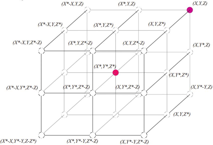
Figure 3: Position vectors along with possible next locations in two dimensions (2D)
Fig. 3 shows the justification behind Eq. (2) for the sake of a two-dimensional problem. The
location of (X , Y ) of the search agent can be updated by the location of the best record (X ∗ , Y ∗ ),CMC, 2021, vol.67, no.3 3805
which is currently found. Various positions around the best agent can be obtained for the current
location by managing the values of vectors A and C. The possible updating position of search
agent in three-dimensional space are discussed in Fig. 4. Any point of search space located among
key-points can be reachable once the random vector (r) is determined (Fig. 3). That is why Eq. (2)
permits each search agent to update its location in the neighborhood of the current optimal
solution and further simulates encircling the prey.
Figure 4: Position vectors along with possible next locations in three dimensions (3D)
Extension of this approach is implied to search space having n dimensions and search agents
continue their movement in hyper-cubes around optimal solution acquired till that time. It has
been mentioned previously that humpback whales also hunt their prey with bubble-net strategy
and this approach is mathematically calculated as follows.
3.3.2 Bubble-Net Attacking Method (Exploitation Phase)
Two methods are suggested for mathematical modeling of bubble-net behavior shown by
humpback whales.
Shrinking Encircling Mechanism. This behavior is attained by minimizing the value of a in
Eq. (3). The range to which A is fluctuated is also minimized by a. It can be said that a is
a random value in the interval [−a, a] where a is minimized from 2 to 0 over a certain set of
iterations. Setting random values for A in [−1, 1], the new position of a search agent can be
determined anywhere among the actual position of agent and position of current best agent.
Fig. 5 represents attainable positions from (X, Y) to (X∗ , Y∗ ), which are reached by 0 ≤ A ≥ 1 in
a two-dimensional space.
Spiral Updating Position. This technique calculates the distance among the whale’s location
(X, Y) and prey’s location (X∗ , Y∗ ). Afterward, a spiral equation is created between the two
positions to depict the helix-shaped movement of humpback whales as mentioned below:
(t + 1) = D
X · ebl · cos (2π l) + X
∗ (t) (5)3806 CMC, 2021, vol.67, no.3
Figure 5: Shrinking encircling mechanism in bubble-net search
Here D = |X ∗ (t) − X (t) | and it shows the distance of ith whale to prey (most optimal
solution attained so far), b is considered as a constant to determine the shape of a logarithmic
spiral, l is a random number in [−1, 1]. Humpback whales swim in the surroundings of their
targeted prey in circle and spiral-shaped path as well. They show two simultaneous behaviors and
to model them, we suppose that there exists a probability of 50% of both actions being exhibited
by them during optimization. The mathematical model is mentioned below:
X ∗ (t) − A ·D if p < 0.5
X (t + 1) = (6)
D · ebl · cos (2π l) + X ∗ (t) if p ≥ 0.5
where p is a random number between [0, 1]. Humpback whales also look out for prey randomly.
For this kind of search, the mathematical model is discussed below.
can
Search for Prey (Exploration Phase). Similar mechanism based on modification of vector A
be exploited for prey searching (exploration). Humpback whales also perform random searches in
accordance with their respective positions. We can use A with random values greater than one or
less than −1 to get the search agent in moving the state away from reference whale.
Unlike the exploitation phase, the position of the search agent is updated in this phase
according to the randomly picked agent. This approach and |A| > 1 focus on exploration and
allow the WOA algorithm to conduct global search. The mathematical model is mentioned below:
−−−→
D = C · Xrand − X (7)
This algorithm begins with a set of random solutions. In all iterations, search agents update
their positions with either randomly picked search agent or best solution acquired till that time.
The parameter is minimized from 2 to 0 so that exploration and exploitation can be accommo-
dated. A random search agent is picked when |A| > 1. However, the most optimal solution is
chosen when |A| < 1 for updating the locations of search agents. WOA can switch among spiral
and
X (t + 1) = −
−−→
Xrand − A ·D (8)CMC, 2021, vol.67, no.3 3807
−−−→
where, Xrand is a random position vector picked from the existing population. Some possible posi-
tions of a particular solution with A > 1 are mentioned in Fig. 5. circular movement depending
on the value of p. On reaching the satisfactory termination criteria, WOA terminates. From a
theoretical point of view, it can be said that WOA is a global optimizer as it incorporates both
exploration and exploitation capabilities. Moreover, the proposed hyper-cube technique determines
a search in the neighborhood of the optimal solution and allows other search agents to make use
of the best record at present in that domain. Adaptive variation of search vector A allows this
algorithm to transit between exploration and exploitation (by minimizing A, some iterations are
≥ 1 and others are for exploitation |A|
specified for exploration |A| < 1) without any difficulty. It is
also noteworthy that WOA has only two major parameters that require adjustment (A and C).
In this research work, the amount of heuristics and the number of internal parameters are
minimized and therefore, ended up implementing the basic category of WOA algorithm. However,
hybridization with evolutionary search schemes can be the domain of future work.
4 Experimental Results and Analysis
The simulation parameters have been presented in Tab. 1. In this section, the results are
presented from different perspectives like grid size, transmission range, and number of nodes.
Table 1: Simulation parameters
Parameters Values
Population size (particles) 100
Maximum iterations 150
Inertia weight, W 0.694
Lower bound (lb) 0
Upper bound 100
Dimensions 2
Transmission range 1–10 m
Mobility model Random waypoint
Simulation runs 10
W1 (weight of first objective function) 0.5
W2 (weight of second objective function) 0.5
Nodes 20–160
The experiments are conducted on MATLAB for different grid sizes and the results are
compared with ACO, GWO, and DFA. The number of clusters are formed against different trans-
mission ranges from 1 to 10. The simulations are also carried out for different number of nodes
20, 40, 60 and 80. The WOA shows the minimum cost for all the number of nodes. The graphical
results in Figs. 6 and 7. show the superiority in terms of cost reduction for various transmission
ranges for 100 m × 100 m grid size. The results presented in Fig. 8. is for 200 m × 200 m grid
size. These results also show that the proposed algorithm is the most cost-effective algorithm for
communication. There is a distinctive relationship between the transmission range and the number
of clusters. The parameters for both the number of clusters and transmission range are inversely
proportional to each other, which means that by decreasing the transmission range, the number
of clusters of the entire network increases and vice versa. The number of clusters also have an3808 CMC, 2021, vol.67, no.3
impact on network resources, which means that the increase in the number of clusters increases
the required resources.
Nodes = 20 Nodes 40
16 35
ACO ACO
GWO GWO
14 WOA WOA
DFA 30 DFA
12
25
10
Cluster Heads
Cluster Heads
8 20
6
15
4
10
2
0 5
1 2 3 4 5 6 7 8 9 10 1 2 3 4 5 6 7 8 9 10
Transmission Range Transmission Range
Nodes = 60 Nodes = 80
55 80
ACO ACO
50 GWO GWO
WOA 70 WOA
DFA DFA
45
60
40
Cluster Heads
Cluster Heads
50
35
40
30
30
25
20
20
15 10 1
1 2 3 4 5 6 7 8 9 10 2 3 4 5 6 7 8 9 10
Transmission Range Transmission Range
Figure 6: Transmission range vs. CHs for nodes 20–80 grid 100 m × 100 m
Another experiment is conducted considering 300 m × 300 m grid size for the 20 to 60 nodes.
The results presented in Fig. 10 also show that the proposed WOA still performs better compared
to other algorithms for the given scenarios. It can also be observed from the results that the
proposed algorithm optimizes the routing by efficient clustering, which reduces the number of
hopes for network communication. This ultimately minimize the packet delay and routing cost.
This is because fewer resources will be required for a lesser number of clusters. All the experiments
compare the results of the proposed WOA with other methods for fallout. Figs. 6–10 shows thatCMC, 2021, vol.67, no.3 3809
WOA considerably show better results as compared to other mentioned algorithms. The results
justify the relationship between transmission range and the number of clusters, the resources
required for the number of clusters. This optimization ultimately reduces the routing cost for
the network.
120
Nodes 120
100
Nodes = 100
ACO
110 GWO
ACO WOA
90 GWO DFA
WOA
DFA 100
80
90
70
Cluster Heads
Cluster Heads
80
60 70
60
50
50
40
40
30
30
20 20
1 2 3 4 5 6 7 8 9 10 1 2 3 4 5 6 7 8 9 10
Transmission Range Transmission Range
Nodes = 140 Nodes = 160
120 140
ACO ACO
110 GWO
WOA 130 GWO
WOA
DFA DFA
100
120
90
110
Cluster Heads
Cluster Heads
80
100
70
90
60
80
50
70
40
30 60
20 50
1 2 3 4 5 6 7 8 9 10 1 2 3 4 5 6 7 8 9 10
Transmission Range Transmission Range
Figure 7: Transmission range vs. CHs for nodes 100–160 grid 100 m × 100 m3810 CMC, 2021, vol.67, no.3
Nodes = 20 Nodes 40
16 35
ACO
ACO GWO
14 GWO WOA
WOA DFA
DFA
30
12
10
Cluster Heads
Cluster heads
25
8
6 20
4
15
2
0
1 2 3 4 5 6 7 8 9 10 10
1 2 3 4 5 6 7 8 9 10
Transmission Range
Transmission Range
Nodes= 60 Nodes= 80
60 80
ACO
55 GWO ACO
WOA GWO
DFA 70 WOA
DFA
50
60
45
Cluster Heads
Cluster Heads
40 50
35
40
30
30
25
20 20
15
1 2 3 4 5 6 7 8 9 10 10
1 2 3 4 5 6 7 8 9 10
Transmission Range Transmission Range
Figure 8: Transmission range vs. CHs for nodes 20–80 grid 200 m × 200 m
The results in Fig. 6 shows that WOA form fifteen clusters initially and then move to fifty-
four clusters for 60 nodes, which shows better performance in terms of optimized clusters for
transmission range of 1 meter. The detailed analysis for 200 m × 200 m grid is shown in Fig. 8.
Fig. 8 shows that the proposed algorithm performs better than other mentioned algorithms.
Fig. 10 shows the results for 300 m × 300 m grid for 1 to 10 transmission ranges. By comparing
the results of Figs. 8 and 9, it is evident that number of clusters increases by increasing grid size.
This shows a direct relation between grid size and the number of clusters. The next experiment is
conducted with 200 m × 200 m grid size and taking transmission range from 1 to 10. The distance
between nodes increases by increasing the grid size, which shows a direct relation and ultimatelyCMC, 2021, vol.67, no.3 3811
increases in grid size isolate the nodes. The increase in a high number of isolated nodes, which
results in the maximum number of clusters for each mentioned algorithm. It can be observed
from Figs. 6 and 7 that the algorithms GWO and WOA produced the same number of clusters.
However, the proposed WOA still performs better compared to the other algorithms and reduces
the number of clusters by 46%. Therefore, we can conclude that the relationship between the
transmission range and the number of clusters is inversely proportional. Therefore, the number of
clusters decreases by increasing the transmission range. This is because many clusters are required
to cover a large area. However, it is still observed that the proposed algorithm produced a smaller
number of clusters compared to other mentioned algorithms. The overlap of the proposed and
other mentioned algorithms on some points is due to the randomness, which is because of the
random nature of evolutionary algorithms.
Nodes= 100 Nodes= 120
100 120
ACO ACO
90 GWO 110 GWO
WOA WOA
DFA DFA
100
80
90
70
Cluster Heads
Cluster heads
80
60
70
50
60
40
50
30 40
20 30
1 2 3 4 5 6 7 8 9 10 1 2 3 4 5 6 7 8 9 10
Transmission Range Transmission Range
Nodes 140 Nodes= 160
140 160
ACO ACO
130 GWO 150 GWO
WOA WOA
DFA DFA
140
120
130
110
120
Cluster Heads
Cluster Head
100
110
90
100
80
90
70
80
60 70
50 60
1 2 3 4 5 6 7 8 9 10 1 2 3 4 5 6 7 8 9 10
Transmission Range Transmission Range
Figure 9: Transmission range vs. CHs for nodes 100–160 grid 200 m × 200 m3812 CMC, 2021, vol.67, no.3
Nodes = 20 Nodes =60
20 65
ACO ACO
GWO 60 GWO
WOA WOA
DFA DFA
55
50
15
Cluster Heads
45
Cluster Head
40
35
10
30
25
20
15
5 1 2 3 4 5 6 7 8 9 10
1 2 3 4 5 6 7 8 9 10
Transmission Range
Transmission Range
N = 100 Nodes = 160
100 180
ACO ACO
GWO GWO
90 WOA WOA
DFA 160 DFA
80
140
70
Cluster Heads
Cluster Heads
60 120
50
100
40
80
30
20 60
0 2 4 6 8 10 1 2 3 4 5 6 7 8 9 10
Transmission Range Transmission Range
Figure 10: Transmission range vs. CHs for nodes 20–160 grid 300 m × 300 m
5 Conclusion
There are various BODYNETs algorithms proposed in the literature for cluster optimization.
These algorithms have their strengths and weaknesses for network resource utilization. The pro-
posed work for node clustering is inspired by the nature of whales. It performs better than the
GWO, ACO, and DFA in terms of the number of CHs for varying transmission ranges, grid
size, and number of nodes. It reduces the communication cost of the network by minimizing the
number of clusters. This minimized number of clusters also leads to less resource requirements in
BODYNETS. In the future, we intend to design an objective function based on user requirements.CMC, 2021, vol.67, no.3 3813
This can further be extended to multi-objective functions as well. The proposed work can also be
modified for dynamic transmission ranges for nodes.
Funding Statement: This work was supported by the National Research Foundation of Korea
(NRF) grant funded by the Korea Government (MSIT) (No. NRF-2018R1C1B5038818).
Conflicts of Interest: The authors declare that they have no conflicts of interest to report regarding
the present study.
References
[1] G. Z. Yang, J. Andreu-Perez, X. Hu and S. Thiemjarus, “Multi-sensor fusion,” in Body Sensor Networks,
London: Springer, pp. 301–354, 2014.
[2] G. Fortino, R. Giannantonio, R. Gravina, P. Kuryloski and R. Jafari, “Enabling effective programming
and flexible management of efficient body sensor network applications,” IEEE Transactions on Human-
Machine Systems, vol. 43, no. 1, pp. 115–133, 2013.
[3] H. Liao, Z. Zhou, X. Zhao, L. Zhang, S. Mumtaz et al., “Learning-based context-aware resource
allocation for edge-computing-empowered industrial IoT,” IEEE Internet of Things Journal, vol. 7, no. 5,
pp. 4260–4277, 2020.
[4] A. Musaddiq, Y. B. Zikria, O. Hahm, H. Yu, A. K. Bashir et al., “A survey on resource management
in IoT operating systems,” IEEE Access, vol. 6, pp. 8459–8482, 2018.
[5] A. N. Alvi, S. Khan, M. A. Javed, K. Konstantin, A. O. Almagrabi et al., “OGMAD: Optimal GTS-
allocation mechanism for adaptive data requirements in IEEE 802.15.4 based internet of things,” IEEE
Access, vol. 7, pp. 170629–170639, 2019.
[6] G. Fortino, G. Di Fatta, M. Pathan and A. V. Vasilakos, “Cloud-assisted body area networks: State-
of-the-art and future challenges,” Wireless Networks, vol. 20, no. 7, pp. 1925–1938, 2014.
[7] S. Ullah, H. Higgins, B. Braem, B. Latre, C. Blondia et al., “A comprehensive survey of wireless body
area networks,” Journal of Medical Systems, vol. 36, no. 3, pp. 1065–1094, 2012.
[8] R. Gravina, P. Alinia, H. Ghasemzadeh and G. Fortino, “Multi-sensor fusion in body sensor networks:
State-of-the-art and research challenges,” Information Fusion, vol. 35, no. 3, pp. 68–80, 2017.
[9] L. Feng, A. Ali, M. Iqbal, A. K. Bashir and S. A. Hussain, “Optimal haptic communications
over nanonetworks for E-health systems„” IEEE Transactions on Industrial Informatics, vol. 15, no. 5,
pp. 3016–3027, 2019.
[10] J. Bangash, A. Abdullah, M. Anisi and A. Khan, “A survey of routing protocols in wireless body
sensor networks,” Sensors, vol. 14, no. 1, pp. 1322–1357, 2014.
[11] A. Bag and M. A. Bassiouni, “Energy efficient thermal aware routing algorithms for embedded biomed-
ical sensor networks,” in IEEE Int. Conf. on Mobile Ad Hoc and Sensor Systems, Vancouver, BC, Canada,
pp. 604–609, 2006.
[12] A. G. Ruzzelli, R. Jurdak, G. M. O’Hare and P. Van Der Stok, “Energy-efficient multi-hop medical
sensor networking,” in Proc. of the 1st ACM SIGMOBILE Int. Workshop on Systems and Networking
Support for Healthcare and Assisted Living Environments, San Juan, Puerto Rico, pp. 37–42, 2007.
[13] M. Li, W. Lou and K. Ren, “Data security and privacy in wireless body area networks,” IEEE Wireless
Communications, vol. 17, no. 1, pp. 51–58, 2010.
[14] Y. S. Lee, H. J. Lee and E. Alasaarela, “Mutual authentication in wireless body sensor networks
(WBSN) based on Physical Unclonable Function (PUF),” in 9th IEEE Int. Wireless Communications and
Mobile Computing Conf., Sardinia, Italy, pp. 1314–1318, 2013.
[15] S. Movassaghi, M. Abolhasan and J. Lipman, “A review of routing protocols in wireless body area
networks,” Journal of Networks, vol. 8, no. 3, pp. 559–575, 2013.
[16] A. Maskooki, C. B. Soh, E. Gunawan and K. S. Low, “Opportunistic routing for body area network,”
in IEEE Consumer Communications and Networking Conf., Las Vegas, NV, USA, pp. 237–241, 2011.3814 CMC, 2021, vol.67, no.3
[17] M. Quwaider and S. Biswas, “Probabilistic routing in on-body sensor networks with postural disconnec-
tions,” in Proc. of the 7th ACM Int. Sym. on Mobility Management and Wireless Access, Tenerife, Canary
Islands, Spain, pp. 149–158, 2009.
[18] S. Movassaghi, M. Abolhasan and J. Lipman, “Energy efficient thermal and power aware (ETPA) rout-
ing in body area networks,” in 23rd IEEE Int. Sym. on Personal, Indoor and Mobile Radio Communications,
Sydney, NSW, Australia, pp. 1108–1113, 2012.
[19] M. Quwaider and S. Biswas, “DTN routing in body sensor networks with dynamic postural partition-
ing,” Ad Hoc Networks, vol. 8, no. 8, pp. 824–841, 2010.
[20] Q. Tang, N. Tummala, S. K. S. Gupta and L. Schwiebert, “Communication scheduling to mini-
mize thermal effects of implanted biosensor networks in homogeneous tissue,” IEEE Transactions on
Biomedical Engineering, vol. 52, no. 7, pp. 1285–1294, 2005.
[21] A. Bag and M. A. Bassiouni, “Hotspot preventing routing algorithm for delay-sensitive applications of
in vivo biomedical sensor networks,” Information Fusion, vol. 9, no. 3, pp. 389–398, 2008.
[22] S. Movassaghi, M. Abolhasan, J. Lipman, D. Smith and A. Jamalipour, “Wireless body area networks:
A survey,” IEEE Communications Surveys & Tutorials, vol. 16, no. 3, pp. 1658–1686, 2014.
[23] B. Braem, B. Latre, I. Moerman, C. Blondia and P. Demeester, “The wireless autonomous spanning
tree protocol for multihop wireless body area networks,” in 3rd IEEE Annual Int. Conf. on Mobile and
Ubiquitous Systems-Workshops, San Jose, CA, USA, pp. 1–8, 2006.
[24] B. Braem, B. Latré, C. Blondia, I. Moerman and P. Demeester, “Improving reliability in multi-hop
body sensor networks,” in 2nd IEEE Int. Conf. on Sensor Technologies and Applications, Cap Esterel,
France, pp. 342–347, 2008.
[25] X. Liang and I. Balasingham, “A QoS-aware routing service framework for biomedical sensor net-
works,” in 4th IEEE Int. Sym. on Wireless Communication Systems, Trondheim, Norway, pp. 342–
345, 2007.
[26] X. Liang, I. Balasingham and S. S. Byun, “A reinforcement learning based routing protocol with QoS
support for biomedical sensor networks,” in 1st IEEE Int. Sym. on Applied Sciences on Biomedical and
Communication Technologies, Aalborg, Denmark, pp. 1–5, 2008.
[27] T. Watteyne, I. Augé-Blum, M. Dohler and D. Barthel, “Anybody: A self-organization protocol for
body area networks,” in Proc. of the ICST 2nd Int. Conf. on Body Area Networks, Florence, Italy,
p. 6, 2007.
[28] M. Moh, B. J. Culpepper, L. Dung, T. S. Moh, T. Hamada et al., “On data gathering protocols for in-
body biomedical sensor networks,” in IEEE Global Telecommunications Conf. GLOBECOM’05, St. Louis,
MO, USA, vol. 5, pp. 2996, 2005.
[29] F. Aadil, K. B. Bajwa, S. Khan, N. M. Chaudary and A. Akram, “CACONET: Ant colony optimiza-
tion (ACO) based clustering algorithm for VANET,” PloS One, vol. 11, no. 5, pp. e0154080, 2016.
[30] G. Husnain, S. Anwar and F. Shahzad, “Performance evaluation of CLPSO and MOPSO routing
algorithms for optimized clustering in Vehicular ad hoc networks,” in 14th IEEE Int. Bhurban Conf. on
Applied Sciences and Technology, Islamabad, Pakistan, pp. 772–778, 2017.
[31] F. Aadil, W. Ahsan, Z. U. Rehman, P. A. Shah, S. Rho et al., “Clustering algorithm for internet
of vehicles (IoV) based on dragonfly optimizer (CAVDO),” Journal of Supercomputing, vol. 74, no. 9,
pp. 1–26, 2018.
[32] M. Fahad, F. Aadil, S. Khan, P. A. Shah, K. Muhammad et al., “Grey wolf optimization-based
clustering algorithm for vehicular ad-hoc networks,” Computers & Electrical Engineering, vol. 70,
pp. 853–870, 2018.
[33] M. Fahad, F. Aadil, S. Ejaz and A. Ali, “Implementation of evolutionary algorithms in vehicular
ad-hoc network for cluster optimization,” in IEEE Intelligent Systems Conf., London, UK, pp. 137–
141, 2017.
[34] F. Aadil, S. Khan, K. B. Bajwa, M. F. Khan and A. Ali, “Intelligent clustering in vehicular ad hoc
networks,” TIIS, vol. 10, no. 8, pp. 3512–3528, 2016.You can also read