Automatic Acoustic Mosquito Tagging with Bayesian Neural Networks
←
→
Page content transcription
If your browser does not render page correctly, please read the page content below
Automatic Acoustic Mosquito Tagging with
           Bayesian Neural Networks

 Ivan Kiskin( )1[0000−0002−2551−840X] , Adam D. Cobb3[0000−0003−2868−6983] ,
 Marianne Sinka2[0000−0001−7145−3179] , Kathy Willis2[0000−0002−6763−2489] , and
                  Stephen J. Roberts1[0000−0002−9305−9268]
        1
            University of Oxford, Department of Engineering, OX1 3PJ, UK,
                         {ikiskin, sjrob}@robots.ox.ac.uk
            2
              University of Oxford, Department of Zoology, OX1 3SZ, UK,
                  {marianne.sinka, kathy.willis}@zoo.ox.ac.uk
        3
            SRI International, VA 22209, United States, adam.cobb@sri.com

      Abstract. Deep learning models are now widely used in decision-making
      applications. These models must be robust to noise and carefully map
      to the underlying uncertainty in the data. Standard deterministic neural
      networks are well known to be poor at providing reliable estimates of
      uncertainty and often lack the robustness that is required for real-world
      deployment. In this paper, we work with an application that requires
      accurate uncertainty estimates in addition to good predictive perfor-
      mance. In particular, we consider the task of detecting a mosquito from
      its acoustic signature. We use Bayesian neural networks (BNNs) to infer
      predictive distributions over outputs and incorporate this uncertainty as
      part of an automatic labelling process. We demonstrate the utility of
      BNNs by performing the first fully automated data collection procedure
      to identify acoustic mosquito data on over 1,500 hours of unlabelled field
      data collected with low-cost smartphones in Tanzania. We use uncer-
      tainty metrics such as predictive entropy and mutual information to help
      with the labelling process. We show how to bridge the gap between theory
      and practice by describing our pipeline from data preprocessing to model
      output visualisation. Additionally, we supply all of our data and code.
      The successful autonomous detection of mosquitoes allows us to perform
      analysis which is critical to the project goals of tackling mosquito-borne
      diseases such as malaria and dengue fever.

      Keywords: Acoustic machine learning · Bayesian deep learning · Audio
      event detection.

1   Introduction
Vector-borne diseases are responsible for over 700,000 deaths annually [42]. Vec-
tors are living organisms that can transmit infectious pathogens between hu-
mans, or from animals to humans. Dengue, yellow fever and malaria are exam-
ples of such mosquito-borne diseases, with malaria constituting one of the most
severe public health problems in the developing world. While there are many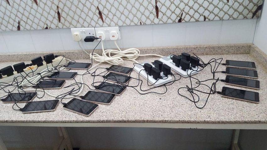
2         I. Kiskin et al.

challenges associated with tackling these diseases, one important task is in in-
formation gathering. In order to respond to large outbreaks quickly and even
predict future ones, it is vital that we develop models that are able to reliably
detect and identify mosquitoes.
    As part of this work, we demonstrate a novel application of Bayesian deep
learning for labelling large amounts of acoustic mosquito data that has been
collected in an unsupervised manner. We showcase that incorporating Bayesian
methods into the tagging process can be extremely beneficial to domain ex-
perts who must eventually check and label data for themselves. As part of the
HumBug project, we have developed an end-to-end pipeline to autonomously
record, detect and archive mosquito sound. Our pipeline utilises conventional
microphones that are found in low-cost mobile phones, and simple adaptions
to bednets already commonly used in malaria-endemic areas [38]. This allows
broad participation, and the possibility of providing a method for widespread
detection in people’s homes. Our work is part of an emerging field where image
and acoustic data is used for building solutions to mosquito control [18, 29, 11,
10]. In order to assist research in methods utilising acoustic event detection or
the study of bioacoustics, we describe our open-source research contributions as
follows:

    – Code: https://github.com/HumBug-Mosquito/MozzBNN. A Bayesian con-
      volutional neural network (BCNN) pipeline for mosquito acoustic event de-
      tection. The model achieves 89 % sensitivity and 97 % specificity on out-
      of-sample test data. We demonstrate how to apply this model to difficult,
      raw, unlabelled field data through filtering predictions by uncertainty met-
      rics intrinsic to probabilistic models. In carefully setting the thresholds of the
      uncertainty metrics, we both avoid missing positive examples of mosquitoes
      in the dataset, as well as avoid the need to manually filter through hundreds
      of hours of data that mostly consists of noise.
    – Data: http://doi.org/10.5281/zenodo.4904800. We provide the output of
      our prediction pipeline applied to a diverse set of acoustic mosquito record-
      ings of over 1,500 hours of uncurated field data. We also supply all the data
      used for training, validating, and testing this model. In total, this forms 20
      hours of mosquito audio recordings expertly labelled with tags precise in
      time, of which 18 hours are annotated with 36 different mosquito species.

    The remainder of the paper is structured as follows. In Section 2.1 we de-
scribe previous mosquito detection efforts, and the context for our contributions.
In Section 2.2 we review related work in acoustic machine learning and Bayesian
deep learning. Section 3.1 describes our full pipeline, breaking down the function
of each component. In Section 3.2, we formally introduce BNNs and the uncer-
tainty metrics which we use for autonomous data collection. Section 4 showcases
our BCNN, detailing the exact architecture, and its parameterisation. In Section
5.1 we show how our model performs on out-of-sample database data, and discuss
our expectation of real-world performance from these results. Section 5.2 shows
how we use uncertainty metrics to evaluate performance of our algorithm over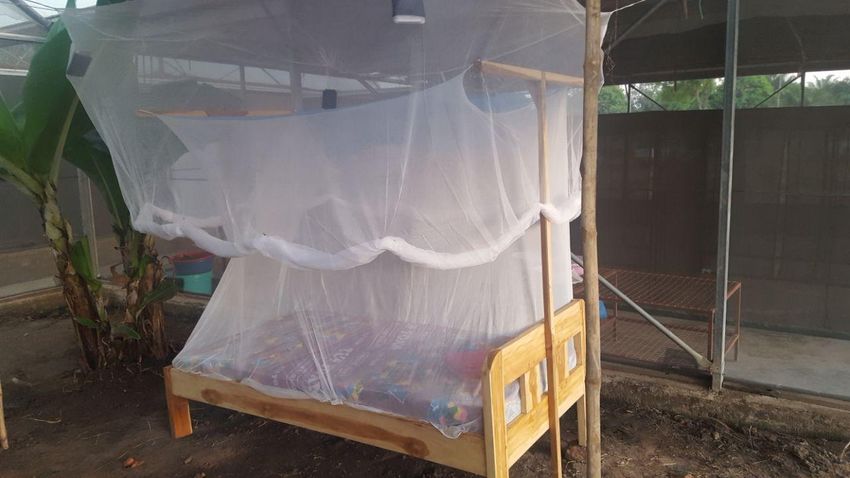
Automatic Acoustic Mosquito Tagging with Bayesian Neural Networks           3

large-scale, real-world, unlabelled data. In Section 6 we identify future directions
and summarise our findings.

2     Background

2.1   Mosquito Control Efforts

Mosquitoes are unique in the way they fly. They have a particularly short, trun-
cated wingbeat allowing them to flap their wings faster than any other insect of
equivalent size – up to 1,000 beats per second [37, 2]. This produces their very
distinct and identifiable flight tone and has led many researchers to try and use
their sound to attract, trap or kill them [33, 16, 15, 11, 30].
    There are over 100 genera of mosquito in the world containing over 3,500
species and they are found on every continent except Antarctica [14]. Only one
genus (Anopheles) contains species capable of transmitting the parasites respon-
sible for human malaria. It contains over 475 formally recognised species of which,
approximately 75 are vectors of human malaria and around 40 are considered
truly dangerous [39]. These 40 species are inadvertently responsible for more
human deaths than any other creature. In 2019, for example, malaria caused
around 229 million cases of disease across more than 100 countries resulting in
an estimated 409,000 deaths [42]. It is imperative therefore to accurately lo-
cate and identify the few dangerous mosquito species amongst the many benign
ones to achieve efficient mosquito control. Mosquito surveys are used to establish
vector species’ composition and abundance, human biting rates and thus the vec-
torial capacity (potential to transmit a pathogen). Traditional survey methods,
such as human landing catches, which collect mosquitoes as they land on the
exposed skin of a collector, can be time consuming, expensive and are limited
in the number of sites they can survey. They can also be subject to collector
bias, either due to variability in the skill or experience of the collector, or in
their inherent attractiveness to local mosquito fauna. These surveys can also
expose collectors to disease. Moreover, once the mosquitoes are collected, the
specimens still need to undergo post-sampling processing for accurate species
identification. Consequently, an affordable automated survey method that de-
tects, identifies and counts mosquitoes could generate unprecedented levels of
high-quality occurrence and abundance data over spatial and temporal scales
currently difficult to achieve.

2.2   Acoustic Machine Learning

Detecting the presence of a mosquito in audio data falls within the broader area
of audio event detection. Within speech recognition, where audio applications
were most common, previous work in applying machine learning techniques has
seen approaches evolve from using Hidden Markov models for making classifica-
tions on phenomes or Mel-frequency cepstral coefficients (MFCCs) [19], to using
convolutional neural networks (CNNs) for end-to-end learning [35]. Similarly to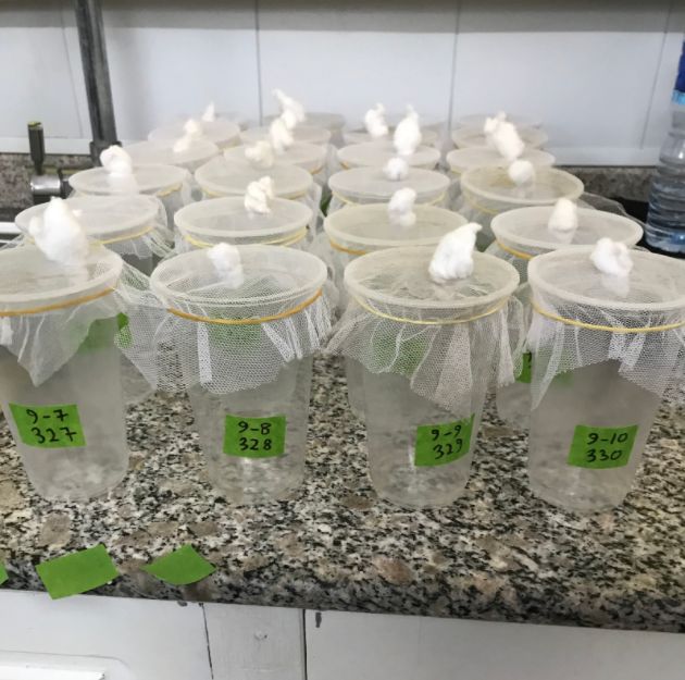
4       I. Kiskin et al.

computer vision, audio event recognition has undergone a paradigm shift from
hand-crafted representations to models which also learn end to end [9]. Recently,
much of the success in this area has been seen from applying CNNs [34, 36], where
the task is to classify signals in the spectral feature space (such as short-time
Fourier and log-mel transforms). Examples of successful applications in audio
event and scene classification tasks can be found in the Detection and Classifica-
tion of Acoustic Scenes and Events (DCASE) challenges of the years 2018 to 2020
[7, 8]. For an event detection tagging-based task in 2018, the top five submissions
were found to commonly utilise the log-mel feature space. Across a range of tasks
in 2020, log-mel energies were overwhelmingly the most commonly used feature
transform in high-ranking submissions [8]. Other feature spaces such as wavelets
[25] have shown potential in acoustic insect classification. However, more work is
to be done before finding computationally viable continuous wavelet transforms
for real-time use. We therefore also utilise log-mel features in our work. We also
use a model similar to the supplied baseline in 2018 Task 2, with elements of the
top-performing models [7], as we would like to deploy a well-tested architecture
for robust model performance in the field.
     The vast majority of acoustic ML works have focused on deterministic ap-
proaches to classification, where uncertainty over predictions is not factored in
(and is not encouraged due to the scoring function of typical ML challenges [20,
7, 8]). While deep learning has become an important tool for machine learning
practitioners, the ability to generalise this tool to a wide range of scientific chal-
lenges is still in its infancy. In particular, we stress the importance of quantifying
the uncertainty associated with the outputs of these models, through the use of
BNNs. It is for this reason that our approach is to use current state-of-the-art
methods to signal classification and place them in a Bayesian framework. The
use of BNNs has not become widespread in audio classification, though recent
applications have emerged [4], and BNNs are growing in interest in parallel ap-
plication domains [12, 5]. As a final point, we will also highlight the option to
use the framework of Bayesian decision theory with Bayesian neural networks
to estimate the risk associated with certain classifications [3]. This is especially
important for mosquito detection, as asymmetrical cost functions for making
classifications are often encountered [26].

3     Methods

3.1   HumBug Pipeline

To showcase our application, we show a schematic of our pipeline in Figure 1.
In the following paragraphs we break down the system by each component.

Capturing Mosquito Acoustic Data on a Smartphone Mosquitoes are
small insects and the physical movement of air caused by their beating wings,
responsible for the high-pitched whine of their flight tone, can easily be lost
within even moderate background noise. Thus, to ensure our smartphones record
Automatic Acoustic Mosquito Tagging with Bayesian Neural Networks 5
MozzWear Mosquito
Central server BNN detection
database
Fig. 1. Project workflow. MozzWear is the mobile phone application used to capture
the audio. The app synchronises to a central server, where audio enters the BNN model.
Successful detections are used to create a curated PostgreSQL database. Information
feeds back to improve the model.
data of high enough quality we needed to complete two steps. First, to develop
an app (MozzWear) to detect and record the mosquito’s flight tone using the
in-built microphone on a smartphone. For the app, we use 16-bit mono PCM
wave audio sampled at 8,000 Hz. These parameters are chosen as a result of prior
work on acoustic low-cost smartphone recording solutions for mosquitoes [27, 22,
25].1 Secondly, we require a means to ensure that a mosquito flies close enough
to the smartphone microphone to capture its flight tone (the adapted bednet).
We have developed an adapted bednet that uses the inherent behaviour of
host-seeking mosquitoes to make them fly close enough to the phone’s internal
microphone to passively record flight tone (Figure 2). Its design is based on
traditional rectangular bednets found across the malaria-endemic world. The
bednet is adapted by the addition of a second outer canopy and a detachable
pocket [38]. The pocket is placed at the highest point of the outer canopy above
the occupant’s head and holds a budget smartphone running the MozzWear
app (Figure 2b). The occupant switches on the app as they enter the bednet at
night. Host-seeking mosquitoes are attracted to the CO2 in the breath of the
occupant and become trapped within the second canopy of the bednet. Here
they naturally migrate to the highest point of the net where their flight tone is
recorded. This design targets night-active mosquito species with a predilection
to feed on humans. These characteristics are common amongst the dominant
malaria vectors in Sub-Saharan Africa.
Central Server Following app recording, the audio is synchronised by the user
to a central server, which performs voice activity detection for removing speech
to preserve privacy. The data then enters the classification engine, in its current
iteration a Bayesian convolutional neural network (BCNN), which we describe in
detail in Sections 3.2 and 4. Positive predictions are then filtered and screened,
and stored in a curated database (Section 5.2). The data is then fed back to
the server to update the model. This pipeline has allowed gradual increase of
complexity in modelling to accommodate for greater availability of training data
through time. We note that our database and algorithms are constantly under-
1
Due to bandwidth requirements in rural areas, our latest version uses 32 kbps AAC.6 I. Kiskin et al.
(a) Bednet with four smartphones positioned to (b) Bednet pockets to
trial the best location for recording mosquitoes. hold smartphones for
recording.
Fig. 2. Deployment in Tanzania (Oct 2020) to trial the effectiveness of acoustic
mosquito detection with low-cost non-invasive measures.
going improvement thanks to the feedback loop in our workflow. Please visit [24]
or the links from Section 1 for the latest versions of the data and models.
Mosquito Database There are a number of variables that influence mosquito
flight tone including the size of the mosquito [41], its age [32] and the air temper-
ature [40]. Thus, in order to develop an algorithm to discern different mosquito
species from their flight tone, a training dataset is needed that captures the nat-
ural variation within a population. We therefore built a database of flight tones
recorded from both laboratory grown and wild captured mosquitoes. Details of
the dataset and a full breakdown of all available metadata, including time of
recording, method of capture, recording device, species, and more are given in
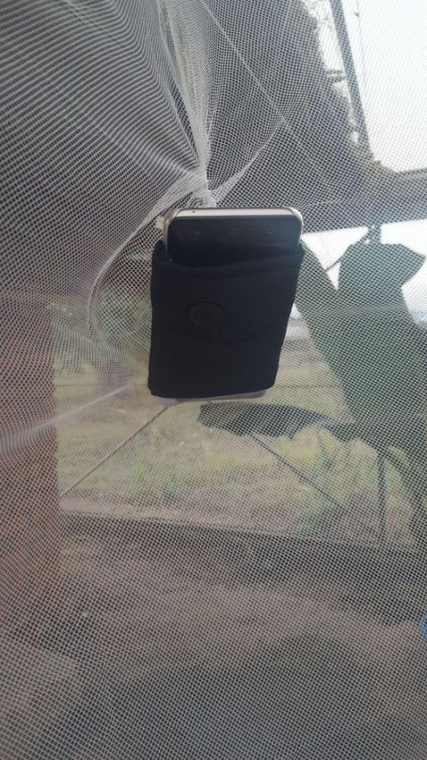
[24]. In summary, live mosquitoes were captured and recorded in Thailand, and
South East Tanzania. To record the mosquito sounds, each captured mosquito
was placed into a sample cup large enough for free flight (Figure 3a) and their
flight tone was recorded using a high specification field microphone (Telinga
EM-23) or a selection of locally available smartphones (Figure 3b) running our
MozzWear app.
We also included in this database flight tone data of multiple species recorded
from laboratory cultures (either free flying in culture cages, or free flying around
bednets as in Figure 2a). These included recordings from the Ifakara Health
Institute, Tanzania, the United States Army Medical Research Unit in Kenya
(USAMRU-K), the Center for Disease Control (CDC) Atlanta, the London
School of Tropical Medicine and Hygiene (LSTMH), and the department of
Zoology at the University of Oxford.
3.2 Bayesian Neural Networks
To provide principled uncertainty estimation for our described pipeline, we re-
quire a model that can provide distributions for each section of audio data.Automatic Acoustic Mosquito Tagging with Bayesian Neural Networks 7
(a) Sample cups used to record wild (b) 16 low-budget Itel A16 smartphones used for
captured mosquitoes. data collection of acoustic bednet data.
Fig. 3. Equipment used in the recording process for curated and field data.
Bayesian neural networks offer a probabilistic alternative to neural networks by
specifying prior distributions over the weights [28, 31]. The placement of a prior
p(ωi ) over each weight ωi leads to a distribution over a parametric set of func-
tions. The motivation for working with BNNs comes from the availability of
uncertainty in its function approximation, f ω (x). When training on a dataset
{X, Y} we want to infer the posterior p(ω|X, Y) over the weights:
p(Y|ω, X)p(ω)
p(ω|X, Y) = . (1)
p(Y|X)
We define the prior p(ω) for each layer l ∈ L as a product of multivariate
QL
normal distributions l=1 N (0, λ−1 l I) (where λl is the prior length-scale) and
the likelihood p(y|ω, x) as a softmax for multi-class (ci ) classification:
exp{fcωi (x)}
p(y = ci |ω, x) = P ω
. (2)
cj exp{fcj (x)}
In testing, the posterior is then required for calculating the predictive distribu-
tion p(y∗ |x∗ , X, Y) for a given test point x∗ . At test time, techniques involving
variational inference (VI) [17] replace the posterior over the weights with a vari-
ational distribution qθ (ω), where we have defined our distribution to depend
on the variational parameters θ. Dropping weights during test time is known
as Monte Carlo (MC) dropout [12] and acts as a test-time approximation for
calculating the predictive distribution. We opt for MC dropout for our models,
as MC dropout provides a cheap approximation of the predictive distribution
without requiring the storage of any additional variational parameters or large
ensembles of network samples.
Having trained a BNN, we have a collection of model weights {ω}Ss=1 for our
MC inference scheme of S dropout samples, but only a single model for a regular
deterministic network. We want the output of our model y∗ to display its confi-
dence in a label. For example, for binary detection, the least confident prediction8 I. Kiskin et al.
would be a vector of [0.5, 0.5]. This vector corresponds to the maximum entropy
prediction, which indicates a high level of uncertainty. On the other hand, a
minimum entropy prediction would be a vector of [1.0, 0.0] or [0.0, 1.0], which
corresponds to the highest confidence possible. For a model displaying any de-
gree of confidence, we would like to verify to which degree this is consistent, and
correct [4]. Therefore, the predictive entropy is a useful way to navigate from
the softmax output to a single value that can indicate the confidence
P of a model
in its prediction. For a deterministic network this is simply − c pc log pc for a
single test input x∗ , where pc is the probability of each class (i.e. each element
in the vector). For the MC approach there are multiple outputs, where each
output corresponds to a different weight sample, ω (s) . There are different ways
to work with the entropy formulation, but we start with the standard solution
which is to average over the outputs and then work with the expected value of
the output. This forms the posterior predictive entropy H̃:
X X
H̃ = − p̃c log p̃c , where p̃c = 1/S p(s)
c . (3)
c s
This does not take into account the origin of the uncertainty (i.e. is it the model
that is unsure, or is the data simply noisy), but for practical purposes it is a
useful tool as it will tell us how much to trust the prediction. However, there
are other ways that we can decompose the uncertainty to distinguish the model
uncertainty from the data uncertainty. For example, it would be helpful to dis-
tinguish between two scenarios that H̃ cannot capture:
A: All samples equally uncertain, e.g. S = 2, y∗ = {[0.5, 0.5], [0.5, 0.5]}
B: All samples are certain, yet fully disagree, e.g. y∗ = {[1.0, 0.0], [0.0, 1.0]}
It might be the case that all the MC samples for the same input result in multi-
ple predictions, with all having the same exact maximum entropy distribution,
[0.5, 0.5]. The H̃ resulting from this scenario would, however, be the same as
sampling two Monte Carlo predictions, where each prediction assigns a 1.0 to
a different class. To distinguish between the two cases, we first introduce the
expectation over the entropy with respect to the parameters E[H]:
X X
E[H] = 1/S h(ω s ), where h(ω) = − pc (ω) log pc (ω). (4)
s c
Now, if we go back to scenario A, H̃ = log 2, E[H] = 0. Let us compare to
scenario B, where H̃ = log 2, but now E[H] = log 2 (see Appendix A). As the
prediction is independent of the samples drawn, the expectation of the entropy
with respect to the weights here is equal to the posterior predictive entropy, and
hence despite sharing the same posterior predictive entropy, the expectations
are not equal. This allows us to determine whether the uncertainty in our model
is due to high disagreement between samples, which could be due to an out of
distribution test point, or whether the model is familiar with the data regime
but correctly shows a higher entropy prediction due to the presence of noise.Automatic Acoustic Mosquito Tagging with Bayesian Neural Networks 9
The mutual information (MI) [13], I(y∗ , ω) between the prediction y∗ and
the model posterior over ω can then be written as:
I(y∗ , ω) = H̃ − E[H]. (5)
The MI will measure how much one variable, say ω, tells us about the other
random variable, say y∗ (or vice-versa). If I(y∗ , ω) = 0, then that tells us that
ω and y∗ are independent, given the data. In the scenario where the predictions
completely disagree with each other for a given x∗ , for each ω s drawn from
the posterior, we get very different predictions. This informs us that y∗ is very
dependent on the posterior draw and thus I(y∗ , ω) = log 2−0 = log 2. However, if
y∗ = [0.5, 0.5] for all ω s ∼ p(ω|Y, X), then the different draws from the posterior
distribution have no effect on the predictive distribution and therefore the mutual
information between the two distributions is zero, as E[H] = h(ω) = H̃ (they
are independent). We therefore use the MI to threshold incoming predictions to
help autonomously label our field data in Section 5.2.
4 Model Configuration
We utilise log-mel spectrogram features for our model input (illustrated in Figure
4 for a particularly loud mosquito sample). It is important to consider how to
parameterise the feature transform, based on trading off frequency and time
resolution, which is a direct result of the Heisenberg uncertainty principle [6]. A
crucial related design decision is the selection of the number of feature windows
that are used to represent a sample, x ∈ Rh×w , where h is the height of the two-
dimensional matrix, and w is the width. The longer the window, w, the better
potential the network has of learning appropriate dynamics, but the smaller
the resulting dataset in number of samples. It may also be more difficult to
learn the salient parts of the sample that are responsible for the signal, resulting
in a weak labelling problem [21]. Early mosquito detection efforts have used
small windows due to a restriction in dataset size. For example, [11] supplies a
rich database of audio, however the samples are limited to just under a second.
However, despite the mosquito’s simple harmonic structure, its characteristic
sound also derives from the temporal variations. We suspect this flight behaviour
tone is better captured over longer windows, since we achieved more robust
results with w = 40, h = 128, corresponding to 40 frames per window, each of
64 ms duration for a total audio slice of 2.56 seconds per sample. We list all
our parameters affecting the feature transformation in Appendix A, Table 2. We
use a BCNN with the architecture as shown in Figure 4. This model structure
is directly based on previous work in mosquito detection. In [25], the authors
demonstrated mosquito detection capability better than that of human domain
experts, when trained on held out recordings within a controlled experiment. In
[22] they also compared a range of 1-D feature vector classifiers (Support Vector
Machines, Random Forests, etc.) and showed that the neural network model gave
the best performance. Therefore we use the same proven model but incorporate
MC dropout at test time. We further increased the size of a training input, and10 I. Kiskin et al.
Dense (15360x128)
Conv2D (3x3x1x32) Conv2D (3x3x32x64)
Input (Nx1x40x128) Output (2)
Dropout Dropout
MaxPool2D MaxPool2D Dropout
Fig. 4. BCNN architecture with tensor dimensions. Log-mel spectrograms are input
with w = 40, h = 128, and passed into two convolutional layers, with 32, and 64,
(3 × 3) kernels of stride 1. Following repeated pooling and dropout, the feature maps
are flattened and fully connected to a dense layer of 128 units, before a final dropout
and softmax output layer. All activation functions are ReLUs, omitted here for clarity.
added an additional convolution and pooling layer due to the greater availability
of data compared to the model used in [23]. The utilisation of dropout layers in
both training and testing produces estimates of uncertainty.
5 Results
5.1 Validation Performance
An important assumption in modelling is that training and test data have been
generated from the same underlying distribution. We aim to train a model which
learns to discriminate classes of that underlying distribution. However, in prac-
tice, due to the myriad of variables that can change for an acoustic recording,
such as the environmental conditions, we find this assumption to not hold true.
As an example, the statistics of noise are varying throughout time by the intro-
duction of novel environments, resulting in non-stationary dynamics. In particu-
lar, consider our binary model of detecting a mosquito signal, and detecting the
absence of signal, i.e. noise. We require a noise class which is representative of the
deployment scenario, which is not known in advance. There are several sources
of noise which we need to address – this can be the noise profile of the recording
devices themselves, as well as the non-stationary environments in which the de-
vices are deployed. We have attempted to mitigate this by collecting data from
a wide range of devices in varying conditions as described in Section 3.1.
We would like to both maximise the data available for training, but also
reserve sufficient data for rigorous evaluation. As of April 2021, our dataset
contains data from 7 experimental setups, and 5 input devices. One strategy
is to hold out entire recordings from each experiment to produce a training
dataset that has sources from each experimental setup. However, training the
model on signal and noise sources for those experiments will allow memorisationAutomatic Acoustic Mosquito Tagging with Bayesian Neural Networks 11
of the signal and noise characteristics. As the samples seen during test time
will very closely approximate those seen in training [25], the model will report
results with accuracy scores that will not be representative of its true predictive
power. Instead, if we have sufficient data to split training and testing into three
experiments used for training, and one held out for testing, we can use a K-
fold cross-validation that withholds entire experiments. We also note that in
practice, these experiments will all contain varying quantities (and quality) of
samples per class, which further complicates issues. We believe there is no one-
size-fits-all approach, and emphasise it is important to understand the sources
of data when designing a model. We opt to hold out two experiments for testing
purposes, and cross-validate our model on the remaining five experiments.
Duration (h) Class acc. (%)
Signal A 2.8 89.27 ± 0.07 Noise 97.24±0.03 2.76±0.03
Noise A 1.3 94.05 ± 0.11 True label
Noise B 3.0 97.99 ± 0.05
Mozz 10.73±0.07 89.27±0.07
(a) Signal A: collation of laboratory
mosquito recording; Noise A: corre-
sponding background. Noise B: En-
ise
zz
Mo
No
vironmental background noise near Predicted label
bednets.
(b) Confusion matrix of (a).
Fig. 5. Out-of-sample performance on held-out test data, estimated with S = 10 MC
dropout samples (mean ± standard deviation).
We collate the test data experiments into the sources of Figure 5 and achieve
a mean classification accuracy of 97 % for the noise class (over 4.3 hours of
data), and 89 % on the mosquito class (over 2.8 hours of data). The standard
deviation is given across 10 MC dropout samples drawn at test time. These class
accuracies would be highly desirable for a model deployed in the field. However,
it is important to consider the process of data labelling. In forming samples for
the BNN input, any audio clip which is shorter than the window length of 2.56
seconds is discarded, and thus the resulting test data only consists of sections that
contain either signal or noise for the entire duration. It is therefore expected to
encounter lower classification accuracy when generalising to new incoming data,
as we do not have guarantees on performance over shorter mosquito events, or if
the sample contains partially noise, and partially mosquito. This can be in part
mitigated by stepping through incoming data, and aggregating neighbouring
predictions to provide resolution at a finer time scale.12 I. Kiskin et al.
5.2 Automatically Labelling Field Data with Uncertainty Metrics
In this section we tackle the challenge of analysing model performance from
data collected at large scale in field studies. To do so, we make use of the open-
source audio editor Audacity [1] to produce an audio-visual output. This serves
as a useful tool for researchers from a range of communities to easily disseminate
results. In the field trial we conducted in Tanzania in November 2020 we gathered
1,500 hours of recordings from 16 mobile phones (Figure 3b). As is common in
biological applications, manually labelling such a dataset is near impossible due
to its size. Algorithm 1 summarises the process by which we pass incoming audio
data through the BNN and then import the audio and predicted labels to screen
detections in Audacity. We format our labels to match the tags used by Audacity.
Figure 6 illustrates the automatic tagging process for one particular section of
recording from the field trial. The upper graphic shows the spectrogram, and
the label track is generated by the BCNN.
Algorithm 1: BCNN detection
for audio file do
Load at 8 kHz;
Calculate sliding window log-mel (40 × 128 frames, each frame 64 ms);
Calculate BCNN predictions with S MC dropout samples;
Calculate mean of p̄c , H, I(y∗ , ω) per section with p̄mosquito > pthreshold ;
ˆ ∗ , ω)};
Write labels as {tstart , tend , p̂c , Ĥ, I(y
end
Fig. 6. BCNN predictions on unlabelled field data (Nov 2020) in Audacity in the form:
ˆ Two windows with mosquito present were correctly identified in this
{p̂mosquito , Ĥ, I}.
section of audio, recorded with the arrangement of Figure 2.
Our probabilistic model allows us to both estimate the presence of a mosquito,
as well as quantify how certain our model is in its predictions. To showcase its ef-
fectiveness on field data collected from South East Tanzania, we vary the thresh-
old of uncertainty and study the performance metrics that result from them. WeAutomatic Acoustic Mosquito Tagging with Bayesian Neural Networks 13
fix the model probability and predictive entropy threshold, and threshold by
the MI, which best captures model confidence, as discussed in Section 3.2. We
vary the MI threshold from its maximum value of 1.0 (log2 (2), Appendix A for
max MI calculation) through a series of discrete steps as given in Table 2. We
calculate the quantity of positives that the model produces for those values, and
estimate the precision and negative predictive value, NPV (which can be thought
of as the precision for the negative class), by manually screening the detections.
Our key result is that the model has well-calibrated uncertainty, as the preci-
Table 1. Effect of mutual information thresholding on the precision and the negative
predictive value (NPV). Positives: duration of audio which was predicted as positive.
Mosquito recovered: duration of the mosquito audio which was recovered from all the
data.
pthreshold Ithreshold (y∗ , ω) NPV Positives Precision Mosquito recovered
0.7 1.0 & 98 % 18h1m 12 % 2h
0.7 0.1 & 99 % 5h30m 30 % 1h39m
0.7 0.05 & 99 % 1h39m 54 % 53m
0.7 0.02 & 99 % 38m 58 % 22m
0.7 0.01 & 99.9 % 20m 60 % 12m
0.7 0.005 & 99.99 % 5m 99 % 5m
sion increases from 12 % to 99 % with the tightening of the mutual information
threshold from 1.0 to 0.005. It also illustrates the problems an equivalent deter-
ministic neural network would have, as a probability threshold of 0.7 on its own
is not sufficient to provide a useful detector, despite showing strong performance
in previous tasks. At the extreme end of confidence, we approach 100 % preci-
sion and negative predictive value, which is a remarkable result from an input
of 1,500 hours of novel data. The trade-off this comes with is a prediction of a
very small quantity of data (low recall). In practice, we would choose a point on
the MI operating curve which balances an acceptable precision and recall of the
model. Following further tweaking based on the results of Table 1, we screened
the predictions with thresholds of p = 0.8, H = 0.5, I = 0.09. The results of this
process have been uploaded to our database in [24], and can be accessed with
the metadata country: Tanzania, location type: field.
6 Conclusion
In this paper we demonstrated how to successfully deploy Bayesian convolutional
neural networks for the automatic identification and labelling of mosquitoes.
We used BCNNs to lessen the burden of manually labelling the rare mosquito
events. The automatic identification of likely mosquitoes reduced the size of the
data required for labelling from 1,500 hours to 18 hours, or less, depending on
the uncertainty threshold. As a result, the challenge of tagging extremely rare14 I. Kiskin et al.
mosquito events was made easier by using the model to correctly identify likely
mosquito events and remove large proportions of the noise.
Key to the success of our implementation was the use of uncertainty metrics.
We used the mutual information to filter through the real-world data and verified
that the model’s precision increased as the mutual information threshold was
reduced. We highlight that the use of the mutual information was only possible
because we used a BNN. Standard neural networks do not provide stochastic
output and therefore do not allow for meaningful measurements of the mutual
information. As a result, the analysis shown in Section 5.2 would not be possible
with deterministic networks.
In conclusion, we are the first to apply Bayesian neural networks in the con-
text of mosquito detection and highlight the utility of estimating the uncertainty
as part of the labelling process. In future work we will continue to explore further
inference schemes for neural networks as well as incorporate Bayesian decision
theory. We also hope to use our pipeline for automatically tagging mosquitoes to
build larger labelled datasets that can then be used to build more sophisticated
models for future real-world field experiments.
A Appendix
Scenario B (samples are certain, yet fully disagree), y∗ = {[1.0, 0.0], [0.0, 1.0]}:
1 X (s) 1 1 1 X (s) 1 1
p̃1 = p1 = (1 + 0) = , p̃2 = p2 = (0 + 1) = , (6)
2 s 2 2 2 s 2 2
1 1 1 1
H̃ = −( log + log ) = log 2, (7)
2 2 2 2
h(1) = −((0) log 0 + (1) log 1) = 0, h(2) = −((1) log 1 + (0) log 0) = 0, (8)
1
E[H] = (0 + 0) = 0, (9)
2
I(y∗ , ω) = H̃ − E[H] = log 2. (10)
Scenario A (all samples equally uncertain), y∗ = {[0.5, 0.5], [0.5, 0.5]}:
1 X (s) 1 1 1 1 1 X (s) 1 1 1 1
p̃1 = p1 = ( + ) = , p̃2 = p2 = ( + ) = , (11)
2 s 2 2 2 2 2 s 2 2 2 2
1 1 1 1
H̃ = −( log + log ) = log 2, (12)
2 2 2 2
E[H] = h(ω) = H̃ = log 2, (13)
I(y∗ , ω) = H̃ − E[H] = 0. (14)Automatic Acoustic Mosquito Tagging with Bayesian Neural Networks 15
Table 2. Feature transformation parameters, in samples. Audio processed with
librosa at 8,000 Hz. The size of 1 frame in w is equal to hop length. For our pa-
rameterisation this is 64 ms, resulting in an input feature slice of w = 2.56 s duration
and h = 128 height.
NFFT win size hop length h (n mels) w Stride
2048 2048 512 128 40 512
Acknowledgements This work has been funded from a 2014 Google Impact
Challenge Award, and has received support from the Bill and Melinda Gates
Foundation (OPP1209888). We would like to thank Paul I Howell and Dustin
Miller (Centers for Disease Control and Prevention, Atlanta), Dr. Sheila Ogoma
(The United States Army Medical Research Unit in Kenya). Prof. Gay Gib-
son (Natural Resources Institute, University of Greenwich) and Dr. Vanessa
Chen-Hussey and James Pearce at the London School of Tropical Medicine and
Hygiene. For significant help and use of their field site Prof. Theeraphap Chare-
onviriyaphap and members of his lab, specifically Dr. Rungarun Tisgratog and
Jirod Nararak (Dept of Entomology, Kasesart University, Bangkok) and Dr.
Michael J. Bangs (Public Health & Malaria Control International SOS Kuala
Kencana, Papua, Indonesia). We also thank NVIDIA for the grant of a Titan
Xp GPU.
References
1. Audacity: Audacity(R): Free audio editor and recorder [computer application]
(2018), https://audacityteam.org/, version 2.2.2 accessed: 2021-01-21
2. Bomphrey, R.J., Nakata, T., Phillips, N., Walker, S.M.: Smart wing rotation and
trailing-edge vortices enable high frequency mosquito flight. Nature 544(7648),
92–95 (2017)
3. Cobb, A.D.: The Practicalities of Scaling Bayesian Neural Networks to Real-World
Applications. Ph.D. thesis, University of Oxford (2020)
4. Cobb, A.D., Jalaian, B.: Scaling Hamiltonian Monte Carlo Inference for Bayesian
Neural Networks with Symmetric Splitting. arXiv preprint arXiv:2010.06772
(2020)
5. Cobb, A.D., Roberts, S.J., Gal, Y.: Loss-calibrated approximate inference in
Bayesian neural networks. arXiv preprint arXiv:1805.03901 (2018)
6. De Bruijn, N.: Uncertainty principles in Fourier analysis. Inequalities 2(1), 57–71
(1967)
7. Detection and Classification of Acoustic Scenes and Events 2018: 2018 re-
sults (2018), http://dcase.community/challenge2018/task-general-purpose-audio-
tagging-results, accessed: 2021-04-01
8. Detection and Classification of Acoustic Scenes and Events 2020: 2020 results
(2020), http://dcase.community/challenge2020/task-acoustic-scene-classification-
results-a, accessed: 2021-04-01
9. Dieleman, S., Schrauwen, B.: End-to-end learning for music audio. In: IEEE In-
ternational Conference on Acoustics, Speech and Signal Processing (ICASSP). pp.
6964–6968 (2014)16 I. Kiskin et al.
10. Dou, Z., Madan, A., Carlson, J.S., Chung, J., Spoleti, T., Dimopoulos, G., Cam-
marato, A., Mittal, R.: Acoustotactic response of mosquitoes in untethered flight
to incidental sound. Scientific Reports 11(1), 1–9 (2021)
11. Fanioudakis, E., Geismar, M., Potamitis, I.: Mosquito wingbeat analysis and classi-
fication using deep learning. In: 2018 26th European Signal Processing Conference
(EUSIPCO). pp. 2410–2414 (2018)
12. Gal, Y., Ghahramani, Z.: Dropout as a Bayesian approximation: representing
model uncertainty in deep learning. In: International Conference on Machine Learn-
ing. pp. 1050–1059 (2016)
13. Gal, Y., Islam, R., Ghahramani, Z.: Deep Bayesian active learning with image
data. In: International Conference on Machine Learning. pp. 1183–1192. PMLR
(2017)
14. Greenwalt, Y.S., Siljeström, S.M., Rose, T., Harbach, R.E.: Hemoglobin-derived
porphyrins preserved in a middle eocene blood-engorged mosquito. Proceedings of
the National Academy of Sciences 110(46), 18496–18500 (2013)
15. Jakhete, S., Allan, S., Mankin, R.: Wingbeat frequency-sweep and visual stimuli for
trapping male Aedes aegypti (Diptera: Culicidae). Journal of medical entomology
54(5), 1415–1419 (2017)
16. Johnson, B.J., Ritchie, S.A.: The siren’s song: exploitation of female flight tones
to passively capture male Aedes aegypti (Diptera: Culicidae). Journal of medical
entomology 53(1), 245–248 (2016)
17. Jordan, M.I., Ghahramani, Z., Jaakkola, T.S., et al.: An Introduction to Varia-
tional Methods for Graphical Models. In: Learning in graphical models, pp. 105–
161. Springer (1998)
18. Joshi, A., Miller, C.: Review of machine learning techniques for mosquito control
in urban environments. Ecological Informatics p. 101241 (2021)
19. Juang, B.H., Rabiner, L.R.: Automatic speech recognition – a brief history of the
technology development. Georgia Institute of Technology and the University of
California 1, 67 (2005)
20. Kaggle: BirdCLEF 2021 - Birdcall Identification (2021), https://www.kaggle.com/
c/birdclef-2021/leaderboards, accessed: 2021-04-01
21. Kiskin, I., Meepegama, U., Roberts, S.: Super-resolution of time-series labels for
bootstrapped event detection. Time-series Workshop at the International Confer-
ence on Machine Learning (2019)
22. Kiskin, I., Orozco, B.P., Windebank, T., Zilli, D., Sinka, M., Willis, K., Roberts, S.:
Mosquito detection with neural networks: the buzz of deep learning. arXiv preprint
arXiv:1705.05180 (2017)
23. Kiskin, I., Wang, L., Cobb, A., et al.: Humbug Zooniverse: a crowd-sourced acous-
tic mosquito dataset. International Conference on Acoustics, Speech, and Signal
Processing 2020, NeurIPS Machine Learning for the Developing World Workshop
2019 (2019, 2020)
24. Kiskin, I., Wang, L., Sinka, M., Willis, K., Cobb, A.D., Gutteridge, B., Zilli, D.,
Rafique, W., Dam, R., Marinos, T., Li, Y., Killeen, G., Msaky, D., Kaindoa, E.,
Roberts, S.J.: HumBugDB: a large-scale acoustic mosquito dataset. Zenodo (Jun
2021). https://doi.org/10.5281/zenodo.4904800
25. Kiskin, I., Zilli, D., Li, Y., Sinka, M., Willis, K., Roberts, S.: Bioacoustic detection
with wavelet-conditioned convolutional neural networks. Neural Computing and
Applications: Special Issue on Deep Learning for Music and Audio (Aug 2018)
26. Li, Y., Kiskin, I., Zilli, D., Sinka, M., Chan, H., Willis, K., Roberts, S.: Cost-
sensitive detection with variational autoencoders for environmental acoustic sens-
ing. NeurIPS Workshop on Machine Learning for Audio Signal Processing (2017)Automatic Acoustic Mosquito Tagging with Bayesian Neural Networks 17
27. Li, Y., Zilli, D., Chan, H., Kiskin, I., Sinka, M., Roberts, S., Willis, K.: Mosquito de-
tection with low-cost smartphones: data acquisition for malaria research. NeurIPS
Workshop on Machine Learning for the Developing World (2017)
28. MacKay, D.J.: A practical Bayesian framework for backpropagation networks. Neu-
ral Computation 4(3), 448–472 (1992)
29. Minakshi, M., Bharti, P., Chellappan, S.: Identifying mosquito species using smart-
phone cameras. In: 2017 European Conference on Networks and Communications
(EuCNC). pp. 1–6. IEEE (2017)
30. Mukundarajan, H., Hol, F.J.H., Castillo, E.A., Newby, C., Prakash, M.: Using
mobile phones as acoustic sensors for high-throughput mosquito surveillance. eLife
6, e27854 (Oct 2017)
31. Neal, R.M.: Bayesian learning for neural networks. Lecture Notes in Statistics
volume 118 (2012)
32. Ogawa, K., Kanda, T.: Wingbeat frequencies of some anopheline mosquitoes of
East Asia (Diptera: Culicidae). Applied entomology and zoology 21(3), 430–435
(1986)
33. Perevozkin, V.P., Bondarchuk, S.S.: Species specificity of acoustic signals of
malarial mosquitoes of anopheles maculipennis complex. International Journal of
Mosquito Research 2(3), 150–155 (2015)
34. Piczak, K.J.: Environmental sound classification with convolutional neural net-
works. In: 2015 IEEE 25th International Workshop on Machine Learning for Signal
Processing (MLSP). IEEE (2015)
35. Sainath, T.N., Kingsbury, B., Saon, G., Soltau, H., Mohamed, A.r., Dahl, G.,
Ramabhadran, B.: Deep convolutional neural networks for large-scale speech tasks.
Neural Networks 64, 39–48 (2015)
36. Salamon, J., Bello, J.P.: Deep convolutional neural networks and data augmenta-
tion for environmental sound classification. IEEE Signal Processing Letters 24(3),
279–283 (2017)
37. Simões, P.M., Ingham, R.A., Gibson, G., Russell, I.J.: A role for acoustic distor-
tion in novel rapid frequency modulation behaviour in free-flying male mosquitoes.
Journal of Experimental Biology 219(13), 2039–2047 (2016)
38. Sinka, M.E., Zilli, D., Li, Y., Kiskin, I., Kirkham, D., Rafique, W., Wang, L.,
Chan, H., Gutteridge, B., Herreros-Moya, E., Portwood, H., Roberts, S., Willis,
K.J.: HumBug – An Acoustic Mosquito Monitoring Tool for Use on Budget Smart-
phones. Methods in Ecology and Evolution (2021). https://doi.org/10.1111/2041-
210X.13663
39. Sinka, M.E., Bangs, M.J., Manguin, S., Rubio-Palis, Y., Chareonviriyaphap, T.,
Coetzee, M., Mbogo, C.M., Hemingway, J., Patil, A.P., Temperley, W.H., et al.: A
global map of dominant malaria vectors. Parasites & vectors 5(1), 1–11 (2012)
40. Unwin, D., Corbet, S.A.: Wingbeat frequency, temperature and body size in bees
and flies. Physiological Entomology 9(1), 115–121 (1984)
41. Villarreal, S.M., Winokur, O., Harrington, L.: The impact of temperature and
body size on fundamental flight tone variation in the mosquito vector Aedes aegypti
(diptera: Culicidae): Implications for acoustic lures. Journal of Medical Entomology
54(5), 1116–1121 (2017)
42. World Health Organization: Fact Sheet (2020), https://www.who.int/news-room/
fact-sheets/detail/vector-borne-diseases, accessed: 2020-01-26You can also read