CHARACTERIZING STRUCTURAL REGULARITIES OF LABELED DATA IN OVERPARAMETERIZED MODELS
←
→
Page content transcription
If your browser does not render page correctly, please read the page content below
Under review as a conference paper at ICLR 2021

C HARACTERIZING S TRUCTURAL R EGULARITIES OF
L ABELED DATA IN OVERPARAMETERIZED M ODELS
 Anonymous authors
 Paper under double-blind review

                                             A BSTRACT

         Humans are accustomed to environments that contain both regularities and ex-
         ceptions. For example, at most gas stations, one pays prior to pumping, but the
         occasional rural station does not accept payment in advance. Likewise, deep neural
         networks can generalize across instances that share common patterns or structures,
         yet have the capacity to memorize rare or irregular forms. We analyze how individ-
         ual instances are treated by a model via a consistency score. The score characterizes
         the expected accuracy for a held-out instance given training sets of varying size
         sampled from the data distribution. We obtain empirical estimates of this score for
         individual instances in multiple data sets, and we show that the score identifies out-
         of-distribution and mislabeled examples at one end of the continuum and strongly
         regular examples at the other end. We identify computationally inexpensive proxies
         to the consistency score using statistics collected during training. We apply the
         score toward understanding the dynamics of representation learning and to filter
         outliers during training.

1    I NTRODUCTION
Human learning requires both inferring regular patterns that generalize across many distinct examples
and memorizing irregular examples. The boundary between regular and irregular examples can be
fuzzy. For example, in learning the past tense form of English verbs, there are some verbs whose past
tenses must simply be memorized (GO→WENT, EAT→ATE, HIT→HIT) and there are many regular
verbs that obey the rule of appending “ed” (KISS→KISSED, KICK→KICKED, BREW→BREWED,
etc.). Generalization to a novel word typically follows the “ed” rule, for example, BINK→BINKED.
Intermediate between the exception verbs and regular verbs are subregularities—a set of exception
verbs that have consistent structure (e.g., the mapping of SING→SANG, RING→RANG). Note
that rule-governed and exception cases can have very similar forms, which increases the difficulty
of learning each. Consider one-syllable verbs containing ‘ee’, which include the regular cases
NEED → NEEDED as well as exception cases like SEEK → SOUGHT . Generalization from the rule-
governed cases can hamper the learning of the exception cases and vice-versa. For instance, children
in an environment where English is spoken over-regularize by mapping GO→GOED early in the
course of language learning. Neural nets show the same interesting pattern for verbs over the course
of training (Rumelhart & McClelland, 1986).
Memorizing irregular examples is tantamount to building a look-up table with the individual facts
accessible for retrieval. Generalization requires the inference of statistical regularities in the training
environment, and the application of procedures or rules for exploiting the regularities. In deep
learning, memorization is often considered a failure of a network because memorization implies no
generalization. However, mastering a domain involves knowing when to generalize and when not
to generalize, because the data manifolds are rarely unimodal. Consider the two-class problem of
chair vs non-chair with training examples illustrated in Figure 1a. The iron throne (lower left) forms
a sparsely populated mode (sparse mode for short) as there may not exist many similar cases in the
data environment. Generic chairs (lower right) lie in a region with a consistent labeling (a densely
populated mode, or dense mode) and thus seems to follow a strong regularity. But there are many
other cases in the continuum of the two extreme. For example, the rocking chair (upper right) has
a few supporting neighbors but it lies in a distinct neighborhood from the majority of same-label
instances (the generic chairs).

                                                    1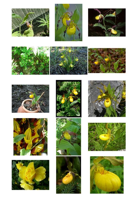
Under review as a conference paper at ICLR 2021
high C-score
(a)
CP,n
AAAB+3icbVBNS8NAFHypX7V+pXr0slgED1ISKeix2IvHCtYW2hA22027dLMJuxulxPwULx4UxKt/xJv/xk3bg7YOLAwz7/FmJ0g4U9pxvq3S2vrG5lZ5u7Kzu7d/YFcP71WcSkI7JOax7AVYUc4E7WimOe0lkuIo4LQbTFqF332gUrFY3OlpQr0IjwQLGcHaSL5dbfnZIMJ6TDDP2vm5yH275tSdGdAqcRekBgu0fftrMIxJGlGhCcdK9V0n0V6GpWaE07wySBVNMJngEe0bKnBElZfNoufo1ChDFMbSPKHRTP29keFIqWkUmMkipVr2CvE/r5/q8MrLmEhSTQWZHwpTjnSMih7QkElKNJ8agolkJisiYywx0aatiinBXf7yKule1N1G3XVvG7Xm9aKPMhzDCZyBC5fQhBtoQwcIPMIzvMKb9WS9WO/Wx3y0ZC12juAPrM8f70qUQA==
regular example
continuum of
sub-regular
examples
low C-score
irregular example
(b) (c)
n=0 n→∞
AAAB63icbVBNS8NAEJ3Ur1q/qh69LBbBU0mkUC9C0YvHitYW2lA220m7dLMJuxuhhP4ELx4UxKt/yJv/xm2bg7Y+GHi8N8PMvCARXBvX/XYKa+sbm1vF7dLO7t7+Qfnw6FHHqWLYYrGIVSegGgWX2DLcCOwkCmkUCGwH45uZ335CpXksH8wkQT+iQ8lDzqix0r28cvvlilt15yCrxMtJBXI0++Wv3iBmaYTSMEG17npuYvyMKsOZwGmpl2pMKBvTIXYtlTRC7WfzU6fkzCoDEsbKljRkrv6eyGik9SQKbGdEzUgvezPxP6+bmvDSz7hMUoOSLRaFqSAmJrO/yYArZEZMLKFMcXsrYSOqKDM2nZINwVt+eZW0L6perep5d7VK4zrPowgncArn4EEdGnALTWgBgyE8wyu8OcJ5cd6dj0VrwclnjuEPnM8fXbyNrA== AAAB/HicbVBNS8NAEN3Ur1q/Yj16WSyCp5JIQY9FLx4rWFtoQtlsN+3SzW7Ynaih9K948aAgXv0h3vw3btsctPXBwOO9GWbmRangBjzv2ymtrW9sbpW3Kzu7e/sH7mH13qhMU9amSijdjYhhgkvWBg6CdVPNSBIJ1onG1zO/88C04UreQZ6yMCFDyWNOCVip71ZloPlwBERr9RhwGUPed2te3ZsDrxK/IDVUoNV3v4KBolnCJFBBjOn5XgrhhGjgVLBpJcgMSwkdkyHrWSpJwkw4md8+xadWGeBYaVsS8Fz9PTEhiTF5EtnOhMDILHsz8T+vl0F8GU64TDNgki4WxZnAoPAsCDzgmlEQuSWEam5vxXRENKFg46rYEPzll1dJ57zuN+q+f9uoNa+KPMroGJ2gM+SjC9REN6iF2oiiJ/SMXtGbM3VenHfnY9FacoqZI/QHzucPfoCVMQ==
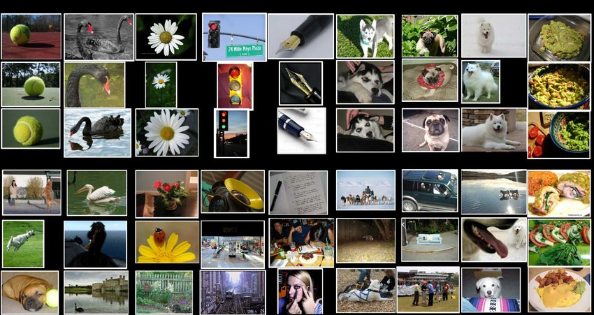
Figure 1: Regularities and exceptions in a binary chairs vs non-chairs problem. (b) illustration of consistency
profiles. (c) Regularities (high C-scores) and exceptions (low C-scores) in ImageNet.
In this article, we study this continuum of the structural regularities of data sets in the context of
n
training overparameterized deep networks. Let D ∼ P be an i.i.d. sample of size n from the
underlying data distribution P, and f (· ; D) be a model trained on D. For an instance x with label y,
we trace out the following consistency profile by increasing n:
CP,n (x, y) = ED∼P
n [P(f (x; D\{(x, y)}) = y], n = 0, 1, . . . (1)
This quantity measures the per-instance generalization on (x, y). For a fixed n, it characterizes how
consistent (x, y) is with a sample D from P. Formally, it is closely tied to the fundamental notion
of generalization performance when we take an expectation over (x, y). Without the expectation,
the quantity gives us a fine-grain characterization of the regularity of each individual example. This
article focuses on classification problems, but the definition can be easily extended to other problems
by replacing the 0-1 classification loss with another suitable loss function.
The quantity CP,n (x, y) has an interpretation that matches our high-level intuition about the structural
regularities of the training data during (human or machine) learning. In particular, we can characterize
the multimodal structure of an underlying data distribution by grouping examples in terms of a
model’s generalization profile for those examples when trained on data sets of increasing size. For
n = 0, the model makes predictions entirely based on its prior belief. As n increases, the model
collects more information about P and makes better predictions. For an (x, y) instance belonging to
a dense mode (e.g., the generic chairs in Figure 1a), the model prediction is accurate even for small n
because even small samples have many class-consistent neighbors. The blue curve in the cartoon
sketch of Figure 1b illustrates this profile. For instances belonging to sparse modes (e.g., the iron
throne in Figure 1a), the prediction will be inaccurate for even large n, as the red curve illustrates.
Most instances fill the continuum between these two extreme cases, as illustrated by the purple curves
in Figure 1b. To obtain a total ordering for all examples, we pool the consistency profile into a scalar
consistency score, or C-score by taking expectation over n. Figure 1c shows examples from the
ImageNet data set ranked by estimated C-scores, using a methodology we shortly describe. The
images show that on many ImageNet classes, there exist dense modes of center-cropped, close-up
shot of the representative examples; and at the other end of the C-score ranking, there exist sparse
modes of highly ambiguous examples (in many cases, the object is barely seen or can only be inferred
from the context in the picture).
With strong ties to both theoretical notions of learning and human intuition, the consistency profile is
an important tool for understanding the regularity and subregularity structures of training data sets
and the learning dynamics of models trained on those data. The C-score based ranking also has many
potential uses, such as detecting out-of-distribution and mislabeled instances; balancing learning
between dense and sparse modes to ensure fairness when learning with data from underrepresented
groups; or even as a diagnostic used to determine training priority in a curriculum learning setting
(Bengio et al., 2009; Saxena et al., 2019). In this article, we focus on formulating and analyzing
consistency profiles, and apply the C-score to analyzing the structure of real world image data sets and
the learning dynamics of different optimizers. We also study efficient proxies and further applications
to outlier detection.
Our key contributions are as follows:
2
Under review as a conference paper at ICLR 2021
Figure 2: Consistency profiles of
ĈD̂,n (x, y)
training examples. Each curve in the
figure corresponds to the average pro-
AAACC3icbZDLSsNAFIYn9VbrLerSTWgRKpSSiKLLYl24rGAv0IQwmU7boZNJmJmIIWTvxldx40IRt76AO9/GSZqFtv4w8PGfc5hzfi+kREjT/NZKK6tr6xvlzcrW9s7unr5/0BNBxBHuooAGfOBBgSlhuCuJpHgQcgx9j+K+N2tn9f495oIE7E7GIXZ8OGFkTBCUynL1qj2FMmmnbpKD7UM5RZAm12naYGn9oRGfuHrNbJq5jGWwCqiBQh1X/7JHAYp8zCSiUIihZYbSSSCXBFGcVuxI4BCiGZzgoUIGfSycJL8lNY6VMzLGAVePSSN3f08k0Bci9j3Vme0qFmuZ+V9tGMnxpZMQFkYSMzT/aBxRQwZGFowxIhwjSWMFEHGidjXQFHKIpIqvokKwFk9eht5p0zpvmrdntdZVEUcZHIEqqAMLXIAWuAEd0AUIPIJn8AretCftRXvXPuatJa2YOQR/pH3+AFtJmzk=
file of a set of examples, partitioned
according to the area under the profile
MNIST Cifar10 Cifar100 curve of each example.
• We formulate and analyze a consistency score that takes inspiration from generalization theory and
matches our high level intuitions.
• We estimate the C-scores with a series of approximations and apply the measure to analyze the
structural regularities of the MNIST, CIFAR-10, CIFAR-100, and ImageNet training sets.
• We demonstrate using C-scores to help analyze the learning dynamics of different optimizers and
consequences for generalization.
• We evaluate a number of learning-speed based measures as efficient proxies for the C-score, and
find that the speed at which an example is learned is a strong indicator of its C-score ranking. While
this observation may be intuitive in retrospect, it is nontrivial because learning speed is measured on
training examples and the C-score is defined for hold-out generalization. An efficiently computable
proxy has practical implications, which we demonstrate with an outlier-detection experiment.
• Because the C-score is generally useful for analyzing data sets and understanding the mechanics of
learning, we have released the pre-computed C-scores at (URL anonymized), together with model
checkpoints, code, and extra visualizations can also be downloaded.
2 R ELATED W ORK
Analyzing the structure of data sets has been a central topic for many fields like Statistics, Data Mining
and Unsupervised Learning. In this paper, we focus on supervised learning and the interplay between
the regularity structure of data and overparameterized neural network learners. This differentiates our
work from classical analyses based on input or (unsupervised) latent representations. The distinction
is especially prominent in deep learning where a supervised learner jointly learns the classifier and
the representation that captures the semantic information in the labels.
In the context of deep supervised learning, Carlini et al. (2018) proposed measures for identifying
prototypical examples which could serve as a proxy for the complete data set and still achieve good
performance. These examples are not necessarily the center of a dense neighborhood, which is
what our high C-score measures. Two prototype measures explored in Carlini et al. (2018), model
confidence and the learning speed, are also measures we examine. Their holdout retraining and
ensemble agreement metrics are conceptually similar to our C-score estimation algorithm. However,
their retraining is a two-stage procedure involving pre-training and fine-tuning; their ensemble
agreement mixes architectures with heterogeneous capacities and ignores labels. Feldman (2020) and
Feldman & Zhang (2020) studied the positive effects of memorization on generalization by measuring
the influence of a training example on a test example, and identifying pairs with strong influences. To
quantify memorization, they defined a memorization score for each (x, y) in a training set as the drop
in prediction accuracy on x when (x, y) is removed. A point evaluation of our consistency profile on
a fixed data size n resembles the second term of their score. A key difference is that we are interested
in the profile with increasing n, i.e. the sample complexity required to correctly predict (x, y).
We evaluate various cheap-to-compute proxies for the C-score and found that the learning speed
has a strong correlation with the C-score. Learning speed has been previously studied in contexts
quite different from our focus on generalization of individual examples. Mangalam & Prabhu (2019)
show that examples learned first are those that could be learned by shallower nets. Hardt et al. (2016)
present theoretical results showing that the generalization gap is small if SGD training completes in
relatively few steps. Toneva et al. (2019) study forgetting (the complement of learning speed) and
informally relate forgetting to examples being outliers or mislabeled. There is a large literature of
criteria with no explicit ties to generalization as the C-score has, but provides a means of stratifying
instances. For example, Wu et al. (2018) measure the difficulty of an example by the number of
residual blocks in a ResNet needed for prediction.
3 T HE CONSISTENCY PROFILE AND THE C- SCORE
The consistency profile (Equation 1) encodes the structural consistency of an example with the
underlying data distribution P via expected performance of models trained with increasingly large
data sets sampled from P. However, it is not possible to directly compute this profile because P is
3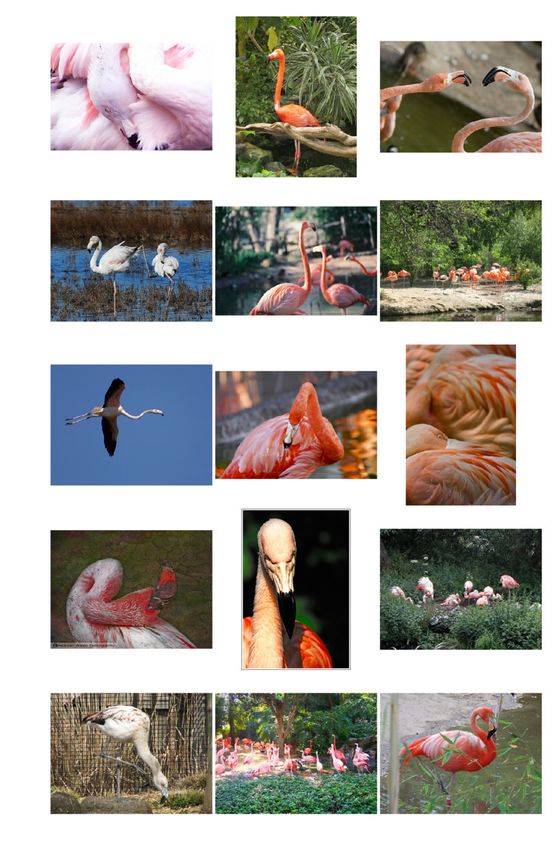
Under review as a conference paper at ICLR 2021
            top ranked examples in CIFAR-10                                     bottom ranked examples with annotations
                                                                                mislabeled       ambiguous         atypical form

                                                                     MNIST
                                                                     CIFAR-10
            top examples in CIFAR-100

                                                                    CIFAR-100
      (a)                                                          (b)

Figure 3: (a) Top ranked examples in CIFAR-10 and CIFAR-100. (b) Bottom ranked examples with annotations.

generally unknown for typical learning problems. In practice, we usually have a fixed data set D̂
consisting of N i.i.d. samples from P. So we can estimate the consistency profile with the following
empirical consistency profile:
                     ĈD̂,n (x, y) = ÊrD∼
                                         n
                                           D̂
                                              [P(f (x; D\{(x, y)}) = y)] ,                    n = 0, 1, . . . N − 1                (2)

where D is a subset of size n uniformly sampled from D̂ excluding (x, y), and Êr denotes empirical
averaging with r i.i.d. samples of such subsets. To obtain a reasonably accurate estimate (say,
r = 1000), calculating the empirical consistency profile is still computationally prohibitive. For
example, with each of the 50,000 training example in the CIFAR-10 training set, we need to train
more than 2 trillion models. To obtain an estimate within the capability of current computation
resources, we make two observations. First, model performance is generally stable when the training
set size varies within a small range. Therefore, we can sample across the range of n that we’re
concerned with and obtain the full profile via smooth interpolation. Second, let D be a random subset
of training data, then the single model f (· ; D) can be reused in the estimation of all of the held-out
examples (x, y) ∈ D̂\D. As a result, with clever grouping and reuse, the number of models we need
to train can be greatly reduced (See Algorithm 1 in the Appendix).
In particular, we sample n dynamically according to the subset ratio s ∈ {10%, . . . , 90%} of the full
available training set. We sample 2,000 subsets for the empirical expectation of each n and visualize
the estimated consistency profiles for clusters of similar examples in Figure 2. One interesting
observation is that while CIFAR-100 is generally more difficult than CIFAR-10, the top ranked
examples (magenta lines) in CIFAR-100 are more likely to be classified correctly when the subset
ratio is low. Figure 3a visualizes the top ranked examples from the two data sets. Note that in
CIFAR-10, the dense modes from the truck and automobile classes are quite similar.
In contrast, Figure 2 indicates that the bottom-ranked examples (cyan lines) have persistently low
probability of correct classification—sometimes below chance—even with a 90% subset ratio. We
visualize some bottom-ranked examples and annotate them as (possibly) mislabeled, ambiguous
(easily confused with another class or hard to identify the contents), and atypical form (e.g., burning
“forest”, fallen “bottle”). As the subset ratio grows, regularities in the data distribution systematically
pull the ambiguous instances in the wrong direction. This behavior is analogous to the phenomenon
we mentioned earlier that children over-regularize verbs (GO→GOED) as they gain more exposure to
a language.
To get a total ordering of the examples in a data set, we distill the consistency profiles into a scalar
consistency score, or C-score, by taking the expectation over n:
                                              ĈD̂ (x, y) = En [ĈD̂,n (x, y)]                                                     (3)

                                                             4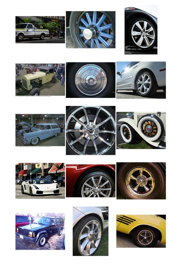
Under review as a conference paper at ICLR 2021
CIFAR-10 MNIST CIFAR-10 CIFAR-100
AAACC3icbZDLSsNAFIYn9VbrLerSTWgRKpSSiKLLYl24rGAv0IQwmU7boZNJmJmIIWTvxldx40IRt76AO9/GSZqFtv4w8PGfc5hzfi+kREjT/NZKK6tr6xvlzcrW9s7unr5/0BNBxBHuooAGfOBBgSlhuCuJpHgQcgx9j+K+N2tn9f495oIE7E7GIXZ8OGFkTBCUynL1qj2FMmmnbpKD7UM5RZAm12naYGn9oRGfuHrNbJq5jGWwCqiBQh1X/7JHAYp8zCSiUIihZYbSSSCXBFGcVuxI4BCiGZzgoUIGfSycJL8lNY6VMzLGAVePSSN3f08k0Bci9j3Vme0qFmuZ+V9tGMnxpZMQFkYSMzT/aBxRQwZGFowxIhwjSWMFEHGidjXQFHKIpIqvokKwFk9eht5p0zpvmrdntdZVEUcZHIEqqAMLXIAWuAEd0AUIPIJn8AretCftRXvXPuatJa2YOQR/pH3+AFtJmzk=
ĈD̂,n (x, y) (a) (b)
AAACCXicbZDLSsNAFIYn9VbrLerSzWARKkhJRNFlsS5cVrAXaEKYTCft0MmFmYkYQrZufBU3LhRx6xu4822cpFlo6w8DH/85hznndyNGhTSMb62ytLyyulZdr21sbm3v6Lt7PRHGHJMuDlnIBy4ShNGAdCWVjAwiTpDvMtJ3p+283r8nXNAwuJNJRGwfjQPqUYykshwdWhMk03bmpAVYPpITjFh6nWVZ4+EkOXb0utE0CsFFMEuog1IdR/+yRiGOfRJIzJAQQ9OIpJ0iLilmJKtZsSARwlM0JkOFAfKJsNPikgweKWcEvZCrF0hYuL8nUuQLkfiu6sw3FfO13PyvNoyld2mnNIhiSQI8+8iLGZQhzGOBI8oJlixRgDCnaleIJ4gjLFV4NRWCOX/yIvROm+Z507g9q7euyjiq4AAcggYwwQVogRvQAV2AwSN4Bq/gTXvSXrR37WPWWtHKmX3wR9rnDw4kmos= AAACCXicbZDLSsNAFIYn9VbrLerSzWARKkhJRNFlsS5cVrAXaEKYTCft0MmFmYkYQrZufBU3LhRx6xu4822cpFlo6w8DH/85hznndyNGhTSMb62ytLyyulZdr21sbm3v6Lt7PRHGHJMuDlnIBy4ShNGAdCWVjAwiTpDvMtJ3p+283r8nXNAwuJNJRGwfjQPqUYykshwdWhMk03bmpAVYPpITjFh6nWVZ4+EkOXb0utE0CsFFMEuog1IdR/+yRiGOfRJIzJAQQ9OIpJ0iLilmJKtZsSARwlM0JkOFAfKJsNPikgweKWcEvZCrF0hYuL8nUuQLkfiu6sw3FfO13PyvNoyld2mnNIhiSQI8+8iLGZQhzGOBI8oJlixRgDCnaleIJ4gjLFV4NRWCOX/yIvROm+Z507g9q7euyjiq4AAcggYwwQVogRvQAV2AwSN4Bq/gTXvSXrR37WPWWtHKmX3wR9rnDw4kmos= AAACCXicbZDLSsNAFIYn9VbrLerSzWARKkhJRNFlsS5cVrAXaEKYTCft0MmFmYkYQrZufBU3LhRx6xu4822cpFlo6w8DH/85hznndyNGhTSMb62ytLyyulZdr21sbm3v6Lt7PRHGHJMuDlnIBy4ShNGAdCWVjAwiTpDvMtJ3p+283r8nXNAwuJNJRGwfjQPqUYykshwdWhMk03bmpAVYPpITjFh6nWVZ4+EkOXb0utE0CsFFMEuog1IdR/+yRiGOfRJIzJAQQ9OIpJ0iLilmJKtZsSARwlM0JkOFAfKJsNPikgweKWcEvZCrF0hYuL8nUuQLkfiu6sw3FfO13PyvNoyld2mnNIhiSQI8+8iLGZQhzGOBI8oJlixRgDCnaleIJ4gjLFV4NRWCOX/yIvROm+Z507g9q7euyjiq4AAcggYwwQVogRvQAV2AwSN4Bq/gTXvSXrR37WPWWtHKmX3wR9rnDw4kmos=
ĈD̂ (x, y) ĈD̂ (x, y) ĈD̂ (x, y)
Figure 4: (a) Histogram of ĈD̂,n for each subset ratio on CIFAR-10. (b) Histogram of the C-score
ĈD̂ averaged over all subset ratios on 3 different data sets.
Figure 5: Examples from MNIST (blocks 1, 2), CIFAR-10 (blocks 3-6), and CIFAR-100 (blocks 7-10). Each
block shows a single class; the left, middle, and right columns of a block depict instances with high, intermediate,
and low C-scores, respectively.
For the case where n is sampled according to the subset ratio s, the expectation is taken over a
uniform distribution over sampled subset sizes.
4 T HE S TRUCTURAL R EGULARITIES OF C OMMON I MAGE DATA S ETS
We apply the C-score estimate to analyze several common image data sets: MNIST, CIFAR-10,
CIFAR-100, and ImageNet. See Appendix A for details on architectures and hyperparameters.
Figure 4a shows the distribution of ĈD̂,n on CIFAR-10 for the values of n corresponding to each
subset ratio s ∈ {10, ..., 90}. For each s, 2000 models are trained and held-out examples are evaluated.
The Figure suggests that depending on s, instances may be concentrated near floor or ceiling, making
them difficult to distinguish (as we elaborate further shortly). By taking an expectation over s,
the C-score is less susceptible to floor and ceiling effects. Figure 4b shows the histogram of this
integrated C-score on MNINT, CIFAR-10, and CIFAR-100. The histogram of CIFAR-10 in Figure 4b
is distributed toward the high end, but is more uniformly spread than the histograms for specific
subset ratios in Figure 4a.
For MNIST, CIFAR-10, and CIFAR-100, Figure 5 presents instances that vary in C-score. Each
block of examples is one category; the left, middle, and right columns have high, intermediate, and
low C-scores, respectively. The homogeneity of examples in the left column suggests dense modes
generally consist of central cropped images of well aligned instances in their typical poses, with
highly uniform color schemes. In contrast, many of the examples in the right column are in atypical
forms or even ambiguous.
Next we apply the C-score analysis to the ImageNet data set. Training a standard model on ImageNet
costs one to two orders of magnitude more computing resources than training on CIFAR, preventing
us from running the C-score estimation procedure described early. Instead, we investigated the
feasibility of approximating the C-score with a point estimate, i.e., selection of the s that best
represents the integral score. This is equivalent to taking expectation of s with respect to a point-mass
distribution, as opposed to the uniform distribution over subset ratios. By ‘best represents,’ we mean
that the ranking of instances by the score matches the ranking by the score for a particular s.
Figure 6a shows the rank correlation between the integral score and the score for a given s, as a
function of s for our three smaller data sets, MNIST, CIFAR-10, and CIFAR-100. Examining the
green CIFAR-10 curve, there is a peak at s = 30, indicating that s = 30 yields the best point-estimate
approximation for the integral C-score. That the peak is at an intermediate s is consistent with
the observation from Figure 2 that the C-score bunches together instances for low and high s. For
MNIST (blue curve), a less challenging data set than CIFAR-10, the peak is lower, at s = 10; for
CIFAR-100 (orange curve), a more challenging data set than CIFAR-10, the peak is higher, at s = 40
5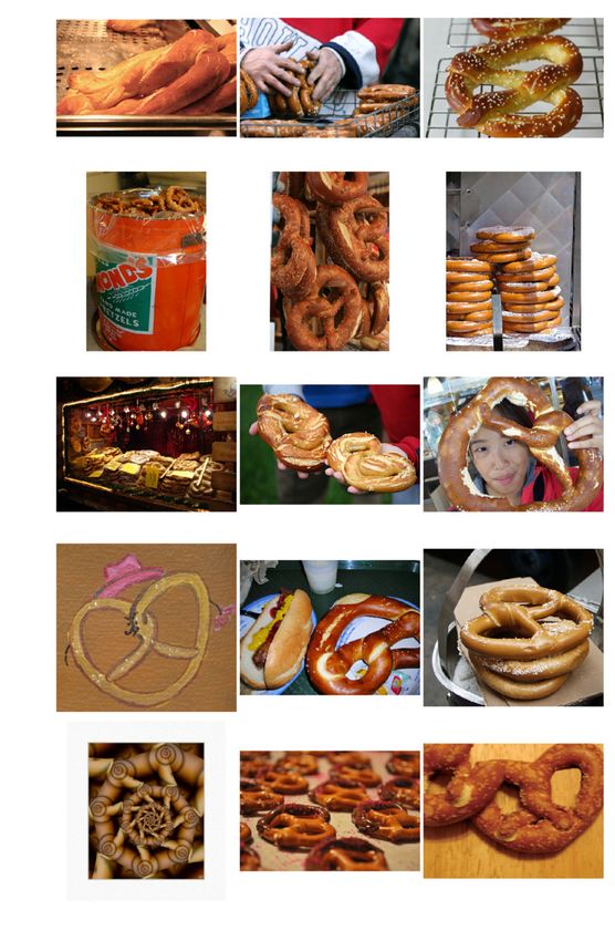
Under review as a conference paper at ICLR 2021

                                                            0.45
                                                                                              car wheel
                                                            0.40

                                                            0.35
                                                                                                          upright                      Figure 6: (a) Rank correlation between integral

                                   Per-class C-score stds
                                                            0.30                                                                       C-score and the C-score for a particular subset
                                                                      projectile
                                                                                                                    school bus
                                                                                                                                       ratio, s. The peak of each curve indicates the
                                                            0.25
                                                                                                                                       training set size that best reveals generalization
                                                            0.20
                                                                                                                                       of the model. (b) Joint distribution of C-score
                                                            0.15
                                                                                                           yellow lady's slipper
                                                                                                                                       per-class means and standard deviations on Ima-
                                                            0.10
                                                                                                                                       geNet. Samples from representative classes (?’s)
                                                                0.2     0.3    0.4    0.5 0.6 0.7 0.8            0.9     1.0
(a)                                (b)                                               Per-class C-scores means                          are shown in Figure 7.

                      projectile          500                            car wheel                                         upright         1000    school bus           1000    yellow lady's slipper
      200                                                                                                  500
       0                                                    0                                                   0                            0                            0
       0.00 0.25 0.50 0.75 1.00                             0.00 0.25 0.50 0.75 1.00                            0.00 0.25 0.50 0.75 1.00     0.00 0.25 0.50 0.75 1.00     0.00 0.25 0.50 0.75 1.00
            C-score Histogram                                    C-score Histogram                                   C-score Histogram            C-score Histogram            C-score Histogram

Figure 7: Example images from ImageNet. The 5 classes are chosen to have representative per-class C-score
mean–standard-deviation profiles, as shown in Figure 6a. For each class, the three columns show sampled
images from the (C-score ranked) top 99%, 35%, and 1% percentiles, respectively. The bottom pane shows the
histograms of the C-scores in each of the 5 classes.

or s = 50. Thus, the peak appears to shift to larger s for more challenging data sets. This finding is
not surprising: more challenging data sets require a greater diversity of training instances in order to
observe generalization.
Based on these observations, we picked s = 70 for a point estimate on ImageNet. In particular, we
train 2,000 ResNet-50 models each with a random 70% subset of the ImageNet training set, and
estimate the C-score based on those models.
The examples shown in Figure 1c are ranked according to this C-score estimate. Because ImageNet
has 1,000 classes, we cannot offer a simple overview over the entire data set as in MNIST and CIFAR.
Instead, we focus on analyzing the behaviors of individual classes. Specifically, we compute the
mean and standard deviation (SD) of the C-scores of all the examples in a particular class. The mean
C-scores indicates the relative difficulty of classes, and the SD indicates the diversity of examples
within each class. The two-dimensional histogram in Figure 6a depicts the joint distribution of mean
and SD across all classes. We selected several classes with various combinations of mean and SD,
indicated by the ?’s in Figure 6a. We then selected sample images from the top 99%, 35% and 1%
percentile ranked by the C-score within each class, and show them in Figure 7.
Projectile and yellow lady’s slipper represent two extreme cases of diverse and unified classes,
respectively. Most other classes lie in the high density region of the 2D histogram in Figure 6b, and
share a common pattern of a densely populated mode of highly regular examples and a tail of rare,
ambiguous examples. The tail becomes smaller from the class car wheel to upright and school bus.

5     A NALYZING L EARNING DYNAMICS WITH THE C- SCORE
In this section, we use the C-score to study the behavior of different optimizers for training deep
neural networks. For this study, we partition the CIFAR-10 training set into subsets by C-score. Then
we record the learning curves—model accuracy over training epochs—for each set. Figure 8 plots the
learning curves for C-score-binned examples. The left panel shows SGD training with a stagewise
constant learning rate, and the right panel shows the Adam optimizer (Kingma & Ba, 2015), which
scales the learning rate adaptively. In both cases, the groups with high C-scores (magenta) generally
learn faster than the groups with low C-scores (cyan). Intuitively, the high C-score groups consist
of mutually consistent examples that support one another during training, whereas the low C-score

                                                                                                                                   6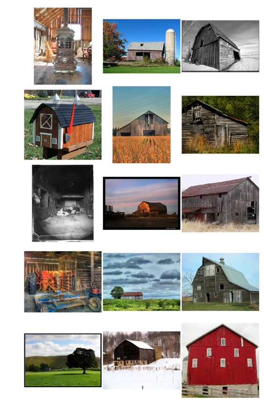
Under review as a conference paper at ICLR 2021
                                  1.0                                                                               1.0

Training accuracy of each group

                                                                                  Training accuracy of each group
                                  0.8                                                                               0.8                                      Figure 8: Learning speed of
                                                          0.00-0.05   0.50-0.55                                                      0.00-0.05   0.50-0.55   CIFAR-10 examples grouped by
                                  0.6                     0.05-0.10   0.55-0.60                                     0.6              0.05-0.10   0.55-0.60
                                                          0.10-0.15   0.60-0.65                                                      0.10-0.15   0.60-0.65   C-score. The thick transpar-
                                                          0.15-0.20   0.65-0.70                                                      0.15-0.20   0.65-0.70
                                  0.4                     0.20-0.25   0.70-0.75                                     0.4              0.20-0.25   0.70-0.75   ent curve shows the average ac-
                                                          0.25-0.30   0.75-0.80                                                      0.25-0.30   0.75-0.80
                                                          0.30-0.35   0.80-0.85                                                      0.30-0.35   0.80-0.85   curacy over the entire training
                                  0.2                     0.35-0.40   0.85-0.90                                     0.2              0.35-0.40   0.85-0.90
                                                          0.40-0.45   0.90-0.95                                                      0.40-0.45   0.90-0.95   set. SGD achieves test accu-
                                                          0.45-0.50   All                                                            0.45-0.50   All
        0.0                                                                              0.0                                                                 racy 95.14%, Adam achieves
            0                             25   50   75 100 125 150 175 200                   0 25                         50   75 100 125 150 175 200
     (a) SGD                                        training epoch                     (b) Adam                                training epoch                92.97%.

groups consist of irregular examples forming sparse modes with fewer consistent peers. In the case
of true outliers, the model needs to memorize the labels individually as they do not share structure
with any other examples.
The learning curves have wider dispersion in SGD than in Adam. Early in SGD training where the
learning rate is large, the examples with the lowest C-scores barely learn. Figure 9a shows SGD with
constant learning rate corresponding to values used in each of the learning rate stages in Figure 8a,
confirming that with a large learning rate, the groups with the lowest C-scores are not learned well
even after the full 200 epochs of training. In comparison, Adam shows less spread among the groups
and as a result, converges sooner. However, the superior convergence speed of adaptive optimizers
like Adam does not always lead to better generalization (Wilson et al., 2017; Keskar & Socher, 2017;
Luo et al., 2019). We observe this outcome as well: SGD with a stagewise learning rate achieves
95.14% test accuracy, compared to 92.97% for Adam.
To develop our intuitions for this phenomenon, we are assisted by the C-score partitioning of examples
in Figure 8. Starting training with a large learning rate effectively enforces a sort of curriculum
in which the model first learns only the strongest regularities. At a later stage when the learning
rate is lowered and exceptions or outliers are able to be learned, the model has already built a solid
representation based on domain regularities. However, when training starts with a small learning rate
or uses Adam to adaptively scale the learning rate, all the examples are learned at similar pace. In this
case, it is difficult to build simple and coherent representations that need to account for all different
modes even in the early stage of learning, which eventually lead to a model with less generalization
power.

 6                                      C- SCORE P ROXIES
We are able to reduce the cost of estimating C-scores from infeasible to feasible, but the procedure is
still very expensive. Ideally, we would like to have more efficient proxies that do not require training
multiple models. We use the term proxy to refer to any quantity that is well correlated with the
C-score but does not have a direct mathematical relation to it, as contrasted with approximations that
are designed to mathematically approximate the C-score (e.g., approximating the expectation with
empirical averaging). The possible candidate set for C-score proxies is very large, as any measure
that reflects information about difficulty or regularity of examples could be considered. Our Related
Work section mentions a few such possibilities. We examined a collection of proxies based on
inter-example distances in input and latent space, but none were terribly promising. (See Appendix
for details.)
Inspired by our observations in the previous section that the speed-of-learning tends to correlate
with the C-score rankings, we instead focus on a class of learning-speed based proxies that have the
added bonus of being trivial to compute. Intuitively, a training example that is consistent with many
others should be learned quickly because the gradient steps for all consistent examples should be
well aligned. One might therefore conjecture that strong regularities in a data set are not only better
learned at asymptote—leading to better generalization performance—but are also learned sooner
in the time course of training. This learning speed hypothesis is nontrivial, because the C-score is
defined for a held-out instance following training, whereas learning speed is defined for a training
instance during training. This hypothesis is qualitatively verified from Figure 8. In particular, the
cyan examples having the lowest C-scores are learned most slowly and the purple examples having
the highest C-scores are learned most quickly. Indeed, learning speed is monotonically related to
C-score bin.
Figure 9b shows a quantitative evaluation, where we compute the Spearman’s rank correlation
between the C-score of an instance and various proxy scores based on learning speed. In particular,
we test accuracy (0-1 correctness), pL (softmax confidence on the correct class), pmax (max softmax
confidence across all classes) and entropy (negative entropy of softmax confidences). We use

                                                                                                                               7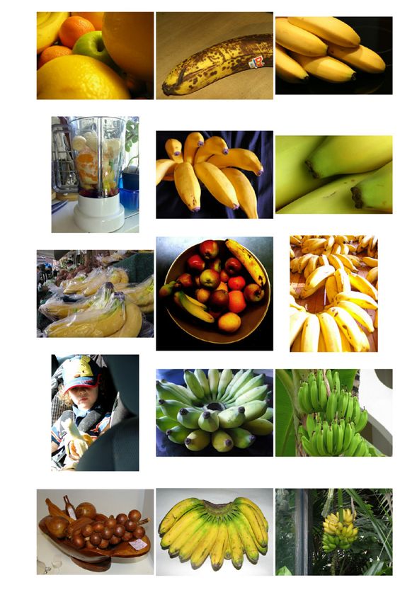
Under review as a conference paper at ICLR 2021

training accuracy per-group
        (a)                                                                   (b)           (c)

Figure 9: (a) Learning speed of CIFAR-10 examples grouped by C-score with SGD using constant
learning rate. The 4 learning rates correspond to the constants in the stage-wise scheduler in Figure 8a.
The test accuracies for those models are 84.84%, 91.19%, 92.05%, and 90.82%, respectively. (b)
Rank correlation (Spearman’s ρ) between C-score and training statistics based proxies. (c) Using
C-score proxies to identify outliers on CIFAR-10.

cumulative statistics which average from the beginning of training to the current epoch because the
cumulative statistics yield a more stable measure—and higher correlation—than statistics based on a
single epoch. We also compare to a forgetting-event statistic (Toneva et al., 2019), which is simply a
count of the number of transitions from “learned” to “forgotten” during training. All of these proxies
show strong correlation with the C-score. pL reaches ρ ≈ 0.9 at the peak. pmax and entropy perform
similarly, both slightly worse than pL . The plot also shows that examples with low cscores are more
likely to be forgotten during training. The forgetting event based proxy slightly under-performs other
proxies and takes a larger number of training epochs to reach its peak correlation. We suspect this is
because forgetting events happen only after an example is learned, so unlike other proxies studied
here, forgetting statistics for hard examples cannot be obtained in the earlier stage of training.
Finally, we present a simple demonstration of the utility of our proxies for outlier detection. We
corrupt a fraction γ = 25% of the CIFAR-10 training set with random label assignments. Then during
training, we identify the fraction γ with the lowest ranking by three C-score proxies—cumulative
accuracy, pL , and forgetting-event statistics. Figure 9c shows the removal rate—the fraction of the
lowest ranked examples which are indeed outliers; two of the C-score proxies successfully identify
over 95% of outliers.

7                             D ISCUSSION

We formulated a consistency profile for individual examples in a data set that reflects the probability
of correct generalization to the example as a function of training set size. This profile has strong
ties to generalization theory and matches basic intuitions about data regularity in both human and
machine learning. We distilled the profile into a scalar C-score, which provides a total ordering of the
instances in a data set by essentially the sample complexity—the amount of training data required—to
ensure correct generalization to the instance. To leverage the C-score to analyze structural regularities
in complex data sets, we derived a C-score estimation procedure and obtained C-scores for examples
in MNIST, CIFAR-10, CIFAR-100, and ImageNet. The C-score estimate helps to characterize the
continuum between a densely populated mode consisting of aligned, centrally cropped examples
with unified shape and color profiles, and sparsely populated modes of just one or two instances. We
also used the C-score as a tool to compare the learning dynamics of different optimizers to better
understand the consequences for generalization. To make the C-score useful in practice for new data
sets, we explored a number of efficient proxies for the C-score based on the learning speed, and found
that the integrated accuracy over training is a strong indicator of an example’s ranking by C-score,
which reflects generalization accuracy had the example been held out from the training set.
In the 1980s, neural nets were touted for learning rule-governed behavior without explicit rules
(Rumelhart & McClelland, 1986). At the time, AI researchers were focused on constructing expert
systems by extracting explicit rules from human domain experts. Expert systems ultimately failed
because the diversity and nuance of statistical regularities in a domain was too great for any human to
explicate. In the modern deep learning era, researchers have made much progress in automatically
extracting regularities from data. Nonetheless, there is still much work to be done to understand
these regularities, and how the consistency relationships among instances determine the outcome of
learning. By defining and investigating a consistency score, we hope to have made some progress in
this direction.

                                                   8
Under review as a conference paper at ICLR 2021

R EFERENCES
Martín Abadi, Ashish Agarwal, Paul Barham, Eugene Brevdo, Zhifeng Chen, Craig Citro, Greg S.
 Corrado, Andy Davis, Jeffrey Dean, Matthieu Devin, Sanjay Ghemawat, Ian Goodfellow, Andrew
 Harp, Geoffrey Irving, Michael Isard, Yangqing Jia, Rafal Jozefowicz, Lukasz Kaiser, Manjunath
 Kudlur, Josh Levenberg, Dandelion Mané, Rajat Monga, Sherry Moore, Derek Murray, Chris Olah,
 Mike Schuster, Jonathon Shlens, Benoit Steiner, Ilya Sutskever, Kunal Talwar, Paul Tucker, Vincent
 Vanhoucke, Vijay Vasudevan, Fernanda Viégas, Oriol Vinyals, Pete Warden, Martin Wattenberg,
 Martin Wicke, Yuan Yu, and Xiaoqiang Zheng. TensorFlow: Large-scale machine learning on
 heterogeneous systems, 2015. URL https://www.tensorflow.org/. Software available
 from tensorflow.org.
Yoshua Bengio, Jérôme Louradour, Ronan Collobert, and Jason Weston. Curriculum learning. In
  Proceedings of the 26th annual international conference on machine learning, pp. 41–48. ACM,
  2009.
Markus M Breunig, Hans-Peter Kriegel, Raymond T Ng, and Jörg Sander. Lof: identifying density-
 based local outliers. In Proceedings of the 2000 ACM SIGMOD international conference on
 Management of data, pp. 93–104, 2000.
Nicholas Carlini, Ulfar Erlingsson, and Nicolas Papernot. Prototypical examples in deep learning:
  Metrics, characteristics, and utility. Technical report, OpenReview, 2018.
Vitaly Feldman. Does learning require memorization? A short tale about a long tail. In ACM
  Symposium on Theory of Computing (STOC), 2020.
Vitaly Feldman and Chiyuan Zhang. What neural networks memorize and why: Discovering the long
  tail via influence estimation. Preprint, 2020.
Moritz Hardt, Ben Recht, and Yoram Singer. Train faster, generalize better: Stability of stochastic
 gradient descent. In International Conference on Machine Learning, pp. 1225–1234. PMLR, 2016.
Arthur Jacot, Franck Gabriel, and Clément Hongler. Neural tangent kernel: Convergence and
  generalization in neural networks. In Advances in neural information processing systems, pp.
  8571–8580, 2018.
Nitish Shirish Keskar and Richard Socher. Improving generalization performance by switching from
  adam to sgd. arXiv preprint arXiv:1712.07628, 2017.
Diederik P Kingma and Jimmy Ba. Adam: A method for stochastic optimization. In International
  Conference on Learning Representations, 2015.
Liangchen Luo, Yuanhao Xiong, Yan Liu, and Xu Sun. Adaptive gradient methods with dynamic
  bound of learning rate. In International Conference on Learning Representations, 2019.
Karttikeya Mangalam and Vinay Uday Prabhu. Do deep neural networks learn shallow learnable
  examples first? In ICML 2019 Workshop on Identifying and Understanding Deep Learning
  Phenomena, 2019.
Alec Radford, Jeffrey Wu, Rewon Child, David Luan, Dario Amodei, and Ilya Sutskever. Language
  models are unsupervised multitask learners. OpenAI Blog, 1(8):9, 2019.
D. E. Rumelhart and J. L. McClelland. On Learning the Past Tenses of English Verbs, pp. 216–271.
  MIT Press, Cambridge, MA, USA, 1986.
Shreyas Saxena, Oncel Tuzel, and Dennis DeCoste. Data parameters: A new family of parameters
  for learning a differentiable curriculum. In H. Wallach, H. Larochelle, A. Beygelzimer, F. d'Alché-
  Buc, E. Fox, and R. Garnett (eds.), Advances in Neural Information Processing Systems 32, pp.
  11093–11103. Curran Associates, Inc., 2019.
Tyler Scott, Karl Ridgeway, and Michael C Mozer. Adapted deep embeddings: A synthesis of methods
  for k-shot inductive transfer learning. In S. Bengio, H. Wallach, H. Larochelle, K. Grauman,
  N. Cesa-Bianchi, and R. Garnett (eds.), Advances in Neural Information Processing Systems 31,
  pp. 76–85. Curran Associates, Inc., 2018.

                                                 9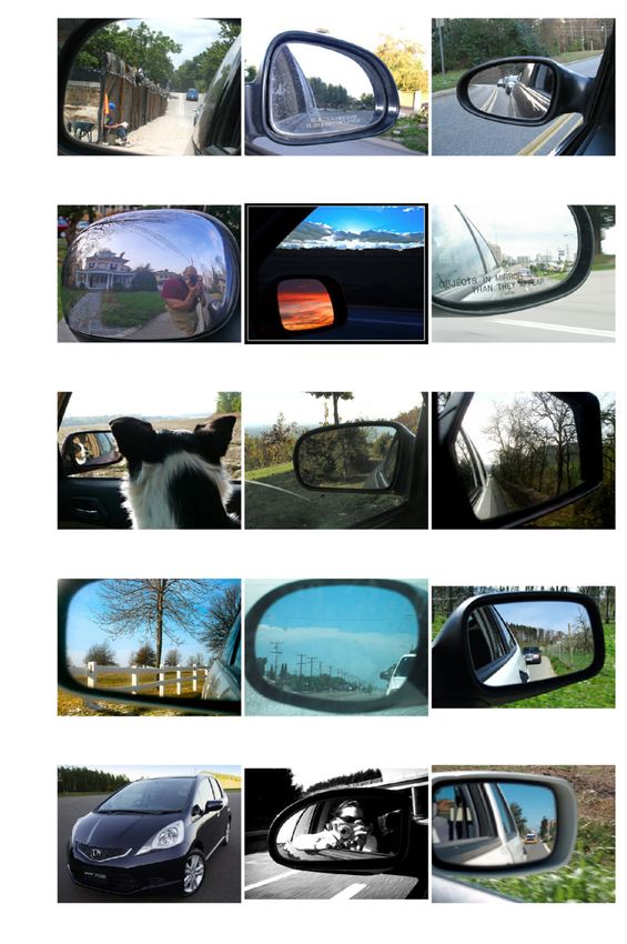
Under review as a conference paper at ICLR 2021

Mingxing Tan and Quoc V Le. Efficientnet: Rethinking model scaling for convolutional neural
 networks. arXiv preprint arXiv:1905.11946, 2019.
Mariya Toneva, Alessandro Sordoni, Remi Tachet des Combes, Adam Trischler, Yoshua Bengio, and
 Geoffrey J Gordon. An empirical study of example forgetting during deep neural network learning.
 In International Conference on Learning Representations, 2019.
Ashia C Wilson, Rebecca Roelofs, Mitchell Stern, Nati Srebro, and Benjamin Recht. The marginal
  value of adaptive gradient methods in machine learning. In Advances in Neural Information
  Processing Systems, pp. 4148–4158, 2017.
Zuxuan Wu, Tushar Nagarajan, Abhishek Kumar, Steven Rennie, Larry S Davis, Kristen Grauman,
  and Rogerio Feris. Blockdrop: Dynamic inference paths in residual networks. In Proceedings of
  the IEEE Conference on Computer Vision and Pattern Recognition, pp. 8817–8826, 2018.

                                              10
Under review as a conference paper at ICLR 2021
A E XPERIMENT D ETAILS
The details on model architectures, data set information and hyper-parameters used in the experiments
for empirical estimation of the C-score can be found in Table 1. We implement our experiment
in Tensorflow (Abadi et al., 2015). The holdout subroutine used in C-score estimation is listed in
Algorithm 1. Most of the training jobs for C-score estimation are run on single NVidia® Tesla P100
GPUs. The ImageNet training jobs are run with 8 P100 GPUs using single-node multi-GPU data
parallelization.
The experiments on learning speed are conducted with ResNet-18 on CIFAR-10, trained for 200
epochs while batch size is 32. For optimizer, we use the SGD with the initial learning rate 0.1,
momentum 0.9 (with Nesterov momentum) and weight decay is 5e-4. The stage-wise constant
learning rate scheduler decrease the learning rate at the 60th, 90th, and 120th epoch with a decay
factor of 0.2.
Algorithm 1 Estimation of ĈD̂,n
Input: Data set D̂ = (X, Y ) with N examples
Input: n: number of instances used for training
Input: k: number of subset samples
Output: Ĉ ∈ RN : (ĈD̂,n (x, y))(x,y)∈D̂
Initialize binary mask matrix M ← 0k×N
Initialize 0-1 loss matrix L ← 0k×N
for i ∈ (1, 2, . . . , k) do
Sample n random indices I from {1, . . . , N }
M [i, I] ← 1
Train fˆ from scratch with the subset X[I], Y [I]
L[i, :] ← 1[fˆ(X) 6= Y ]
end for
Initialize score estimation vector Ĉ ← 0N
for j ∈ (1, 2, . . . , N ) do
Q ← ¬M [:, j]
Ĉ[j] ← sum(¬L[:, Q])/sum(Q)
end for
B T IME AND S PACE C OMPLEXITY
The time complexity of the holdout procedure for empirical estimation of the C-score is O(S(kT +
E)). Here S is the number of subset ratios, k is number of holdout for each subset ratio, and T is the
average training time for a neural network. E is the time for computing the score given the k-fold
holdout training results, which involves elementwise computation on a matrix of size k × N , and is
negligible comparing to the time for training neural networks. The space complexity is the space for
training a single neural network times the number of parallel training jobs. The space complexity for
computing the scores is O(kN ).
For kernel density estimation based scores, the most expensive part is forming the pairwise distance
matrix (and the kernel matrix), which requires O(N 2 ) space and O(N 2 d) time, where d is the
dimension of the input or hidden representation spaces.
C M ORE V ISUALIZATIONS OF I MAGES R ANKED BY C- SCORE
Examples with high, middle and low C-scores from a few representative classes of MNIST, CIFAR-10
and CIFAR-100 are show in Figure 5. In this appendix, we depict the results for all the 10 classes of
MNIST and CIFAR-10 in Figure 10 and Figure 11, respectively. The results from the first 60 out of
the 100 classes on CIFAR-100 is depicted in Figure 12. Figure 13 and Figure 14 show more examples
from ImageNet. Please see (URL anonymized) for more visualizations.
11Under review as a conference paper at ICLR 2021
MNIST CIFAR-10 CIFAR-100 ImageNet
Architecture MLP(512,256,10) Inception† Inception† ResNet-50 (V2)
Optimizer SGD SGD SGD SGD
Momentum 0.9 0.9 0.9 0.9
Base Learning Rate 0.1 0.4 0.4 0.1×7
? ? ?
Learning Rate Scheduler ∧(15%) ∧(15%) ∧(15%) LinearRampupPiecewiseConstant??
Batch Size 256 512 512 128×7
Epochs 20 80 160 100
Data Augmentation · · · · · · Random Padded Cropping~ + Random Left-Right Flipping · · · · · ·
Image Size 28×28 32×32 32×32 224×224
Training Set Size 60,000 50,000 50,000 1,281,167
Number of Classes 10 10 100 1000
† A simplified Inception model suitable for small image sizes, defined as follows:
Inception :: Conv(3×3, 96) → Stage1 → Stage2 → Stage3 → GlobalMaxPool → Linear.
Stage1 :: Block(32, 32) → Block(32, 48) → Conv(3×3, 160, Stride=2).
Stage2 :: Block(112, 48) → Block(96, 64) → Block(80, 80) → Block (48, 96) → Conv(3×3,
240, Stride=2).
Stage3 :: Block(176, 160) → Block(176, 160).
Block(C1 , C2 ) :: Concat(Conv(1×1, C1 ), Conv(3×3,C2 )).
Conv :: Convolution → BatchNormalization → ReLU.
? ∧(15%) learning rate scheduler linearly increase the learning rate from 0 to the base learning rate in
the first 15% training steps, and then from there linear decrease to 0 in the remaining training steps.
?? LinearRampupPiecewiseConstant learning rate scheduler linearly increase the learning rate from 0 to
the base learning rate in the first 15% training steps. Then the learning rate remains piecewise constant
with a 10× decay at 30%, 60% and 90% of the training steps, respectively.
~ Random Padded Cropping pad 4 pixels of zeros to all the four sides of MNIST, CIFAR-10, CIFAR-100
images and (randomly) crop back to the original image size. For ImageNet, a padding of 32 pixels is
used for all four sides of the images.
Table 1: Details for the experiments used in the empirical estimation of the C-score.
Figure 10: Examples from MNIST. Each block shows a single class; the left, middle, and right
columns of a block depict instances with high, intermediate, and low C-scores, respectively.
Figure 11: Examples from CIFAR-10. Each block shows a single class; the left, middle, and right
columns of a block depict instances with high, intermediate, and low C-scores, respectively.
12Under review as a conference paper at ICLR 2021
Figure 12: Examples from CIFAR-100. Each block shows a single class; the left, middle, and right
columns of a block depict instances with high, intermediate, and low C-scores, respectively. The first
60 (out of the 100) classes are shown.
13Under review as a conference paper at ICLR 2021
500 teapot barometer banana 1000
500 500
car mirror 1000 flamingo
0 0 0 0 0
0.00 0.25 0.50 0.75 1.00 0.00 0.25 0.50 0.75 1.00 0.00 0.25 0.50 0.75 1.00 0.00 0.25 0.50 0.75 1.00 0.00 0.25 0.50 0.75 1.00
C-score Histogram C-score Histogram C-score Histogram C-score Histogram C-score Histogram
Figure 13: Example images from ImageNet. For each class, the three columns show sampled images from the
(C-score ranked) top 99%, 35%, and 1% percentiles, respectively. The bottom pane shows the histograms of the
C-scores in each of the 5 classes.
pitcher 500 alp pretzel jeep barn
200 500 500 500
0 0 0 0 0
0.00 0.25 0.50 0.75 1.00 0.00 0.25 0.50 0.75 1.00 0.00 0.25 0.50 0.75 1.00 0.00 0.25 0.50 0.75 1.00 0.00 0.25 0.50 0.75 1.00
C-score Histogram C-score Histogram C-score Histogram C-score Histogram C-score Histogram
Figure 14: Example images from ImageNet. For each class, the three columns show sampled images from the
(C-score ranked) top 99%, 35%, and 1% percentiles, respectively. The bottom pane shows the histograms of the
C-scores in each of the 5 classes.
14Under review as a conference paper at ICLR 2021
Ĉ Ĉ L Ĉ ±L Ĉ LOF
CIFAR-10 −0.064 −0.009 0.083 0.103
ρ
CIFAR-100 −0.098 0.117 0.105 0.151
CIFAR-10 −0.042 −0.006 0.055 0.070
τ
CIFAR-100 −0.066 0.078 0.070 0.101
Table 2: Rank correlation between C-score and pairwise distance based proxies on inputs. Measured
with Spearman’s ρ and Kendall’s τ rank correlations, respectively.
D C-S CORE P ROXIES BASED ON PAIRWISE D ISTANCES
We study C-score proxies based on pairwise distances here. 0.6
Intuitively, an example is consistent with the data distri- 0.4
bution if it lies near other examples having the same label. 0.2
Ĉ
0.0 Ĉ L
However, if the example lies far from instances in the same 0.2 Ĉ ±L
class or lies near instances of different classes, one might 0.4
Ĉ LOF
not expect it to generalize. Based on this intuition, we 0.6
0 20 40 60 80
define a relative local-density score: CIFAR-10 Epoch CIFAR-100
N
1 X Figure 15: Spearman rank correlation be-
Ĉ ±L (x, y) = 2(1[y = yi ] − 21 )K(xi , x), (4) tween C-score and distance-based score on
N i=1
hidden representations.
where K(x, x0 ) = exp(−kx − x0 k2 /h2 ) is an RBF kernel with the bandwidth h, and 1[·] is the
indicator function. To evaluate the importance of explicit label information, we study two related
scores: Ĉ L that uses only same-class examples when estimating the local density, and Ĉ that uses all
the neighbor examples by ignoring the labels.
N
1 X
Ĉ L (x, y) = 1[y = yi ]K(xi , x), (5)
N i=1
N
1 X
Ĉ(x) = K(xi , x). (6)
N i=1
We also study a proxy based on the local outlier factor (LOF) algorithm (Breunig et al., 2000), which
measures the local deviation of each point with respect to its neighbours. Since large LOF scores
indicate outliers, we use the negative LOF score as a C-score proxy, denoted by Ĉ LOF (x).
Table 2 shows the agreement between the proxy scores and the estimated C-score. Agreement is
quantified by two rank correlation measures on three data sets. As anticipated, the input-density
score that ignores labels, Ĉ(x), and the class-conditional density, Ĉ L (x, y), have poor agreement.
Ĉ ±L (x, y) and Ĉ LOF are slightly better. However, none of the proxies has high enough correlation to
be useful, because it is very hard to obtain semantically meaningful distance estimations from the
raw pixels.
Since proxies based on pairwise distances in the input space work poorly, we further evaluate the
proxies using the penultimate layer of the network as a representation of an image: Ĉh±L , ĈhL , Ĉh
and ĈhLOF , with the subscript h indicating that the score operates in hidden space. For each score and
data set, we compute Spearman’s rank correlation between the proxy score and the C-score.
In particular, we train neural network models with the same specification as in Table 1 on the full
training set. We use an RBF kernel K(x, x0 ) = exp(−kx−x0 k2 /h2 ), where the bandwidth parameter
h is adaptively chosen as 1/2 of the mean pairwise Euclidean distance across the data set. For the
local outlier factor (LOF) algorithm (Breunig et al., 2000), we use the neighborhood size k = 3. See
Figure 16 for the behavior of LOF across a wide range of neighborhood sizes.
Because the embedding changes as the network is trained, we plot the correlation as a function of
training epoch in Figure 15. For both data sets, the proxy score that correlates best with the C-score
is Ĉh±L (grey), followed by ĈhLOF (brown), then ĈhL (pink) and Ĉh (blue). Clearly, appropriate use of
15Under review as a conference paper at ICLR 2021
0.25 0.20 input space
hidden space
0.15
Spearman's rho
Spearman's rho
0.20
input space
0.15 hidden space 0.10
0.05
0.10
0.00
0 25 50 75 100 0 25 50 75 100
k k
(a) CIFAR-10 (b) CIFAR-100
Figure 16: The Spearman’s ρ correlation between the C-score and the score based on LOF with
different neighborhood sizes.
Figure 17: Examples from CIFAR-10 (left 5 blocks) and CIFAR-100 (right 5 blocks). Each block
shows a single class; the left, middle, and right columns of a block depict instances with top,
intermediate, and bottom ranking according to the relative local density score Ĉ ±L in the input space,
respectively.
labels helps with the ranking. However, our proxy Ĉh±L uses the labels in an ad hoc manner. We will
discuss a more principled measure based on gradient vectors shortly and relate it to the neural tangent
kernel Jacot et al. (2018).
The results reveal interesting properties of the hidden representation. One might be concerned that as
training progresses, the representations will optimize toward the classification loss and may discard
inter-class relationships that could be potentially useful for other downstream tasks (Scott et al., 2018).
However, our results suggest that Ĉh±L does not diminish as a predictor of the C-score, even long
after training converges. Thus, at least some information concerning the relation between different
examples is retained in the representation, even though intra- and inter-class similarity is not very
relevant for a classification model. To the extent that the hidden representation—crafted through a
discriminative loss—preserves class structure, one might expect that the C-score could be predicted
without label reweighting; however, the poor performance of Ĉh suggests otherwise.
Figure 17 and Figure 18 visualize examples in CIFAR-10/CIFAR-100 ranked by the class weighted
local density scores in the input and learned hidden space, respectively. The ranking calculated in the
input space relies heavily on low level features that can be derived directly from the pixels like strong
silhouette. The rankings calculated from the learned hidden space correlate better with C-score,
though the visualization shows that the ranking are sometimes still noisy even for the top ranking
examples (e.g. the class “automobile” in CIFAR-10).
D.1 PAIRWISE D ISTANCE E STIMATION WITH G RADIENT R EPRESENTATIONS
Most modern neural networks are trained with first order gradient descent based algorithms and
variants. In each iteration, the gradient of loss on a mini-batch of training examples evaluated at the
current network weights is computed and used to update the current parameter. Let ∇t (·) be the
function that maps an input-label training pair (the case of mini-batch size one) to the corresponding
16Under review as a conference paper at ICLR 2021
Figure 18: Examples from CIFAR-10 (left 5 blocks) and CIFAR-100 (right 5 blocks). Each block
shows a single class; the left, middle, and right columns of a block depict instances with top,
intermediate, and bottom ranking according to the relative local density score Ĉh±L in the latent
representation space of a trained network, respectively.
gradient evaluated at the network weights of the t-th iteration. Then this defines a gradient based
representation on which we can compute density based ranking scores. The intuition is that in a
gradient based learning algorithm, an example is consistent with others if they all compute similar
gradients.
Comparing to the hidden representations defined the outputs of a neural network layer, the gradient
based representations induce a more natural way of incorporating the label information. In the
previous section, we reweight the neighbor examples belonging to a different class by 0 or -1. For
gradient based representations, no ad hoc reweighting is needed as the gradient is computed on the
loss that has already takes the label into account. Similar inputs with different labels automatically
lead to dissimilar gradients. Moreover, this could seamlessly handle labels and losses with rich
structures (e.g. image segmentation, machine translation) where an effective reweighting scheme is
hard to find. The gradient based representation is closely related to recent developments on Neural
Tagent Kernels (NTK) (Jacot et al., 2018). It is shown that when the network width goes to infinity,
the neural network training dynamics can be effectively approximately via Taylor expansion at the
initial network weights. In other words, the algorithm is effectively learning a linear model on the
nonlinear representations defined by ∇0 (·). This feature map induces the NTK, and connects deep
learning to the literature of kernel machines.
Although NTK enjoys nice theoretical properties, it is challenging to perform density estimation
on it. Even for the more practical case of finite width neural networks, the gradient representations
are of extremely high dimensions as modern neural networks general have parameters ranging from
millions to billions (e.g. Tan & Le, 2019; Radford et al., 2019). As a result, both computation and
memory requirements are prohibitive if a naive density estimation is to be computed on the gradient
representations. We leave as future work to explore efficient algorithms to practically compute this
score.
E W HAT M AKES AN I TEM R EGULAR OR I RREGULAR ?
The notion of regularity is primarily coming from the statistical consistency of the example with the
rest of the population, but less from the intrinsic structure of the example’s contents. To illustrate
this, we refer back to the experiments in Section 5 on measuring the learning speed of groups of
examples generated via equal partition on the C-score value range [0, 1]. As shown in Figure 4b, the
distribution is uneven between high and low C-score values. As a result, the high C-score groups will
have more examples than the low C-score groups. This agrees with the intuition that regularity arises
from high probability masses.
To test whether an example with top-ranking C-score is still highly regular after the density of its
neighborhood is reduced, we redo the experiment, but subsample each group to contain an equal
number (∼ 400) of examples. Then we run training on this new data set and observe the learning
speed in each (subsampled) group. The result is shown in Figure 19, which is to be compared with
the results without group-size-equalizing in Figure 8a in the main text. The following observations
can be made:
1. The learning curves for many of the groups start to overlap with each other.
17You can also read