Deep Reinforcement Learning for Portfolio Optimization using Latent Feature State Space (LFSS) Module
←
→
Page content transcription
If your browser does not render page correctly, please read the page content below
Deep Reinforcement Learning for Portfolio Optimization using Latent
                                                             Feature State Space (LFSS) Module
                                                                                                          Kumar Yashaswi1

                                               Abstract— Dynamic Portfolio optimization is the process of               in financial market applications. Researchers are constantly
                                            distribution and rebalancing of a fund into different financial             working on machine learning techniques that have proven
                                            assets such as stocks, cryptocurrencies, etc, in consecutive                so successful in computer vision, NLP or beating humans
                                            trading periods to maximize accumulated profits or minimize
arXiv:2102.06233v1 [q-fin.PM] 11 Feb 2021

                                            risks over a time horizon. This field saw huge developments                 in chess, etc, in the domain of dynamic financial markets
                                            in recent years, because of the increased computational power               environment.
                                            and increased research in sequential decision making through                   Before the advent of machine learning, most portfolio
                                            control theory. Recently Reinforcement Learning(RL) has been                models were based on variations of Modern Portfolio The-
                                            an important tool in the development of sequential and dynamic              ory(MPT) by Markowitz [6]. These had the drawbacks of
                                            portfolio optimization theory. In this paper, we design a Deep
                                            Reinforcement Learning (DRL) framework as an autonomous                     being static and linear in computation. The dynamic meth-
                                            portfolio optimization agent consisting of a Latent Feature State           ods used for this problem like dynamic programming and
                                            Space(LFSS) Module for filtering and feature extraction of                  convex optimization, required discrete action space based
                                            financial data which is used as a state space for deep RL                   models and thus were not so efficient in capturing market
                                            model. We develop an extensive RL agent with high efficiency                information [7,8]. To address this issue we work with deep
                                            and performance advantages over several benchmarks and
                                            model-free RL agents used in prior work. The noisy and non-                 reinforcement learning model. Reinforcement Learning(RL)
                                            stationarity behaviour of daily asset prices in the financial               is an area in artificial intelligence which focuses on how
                                            market is addressed through Kalman Filter. Autoencoders,                    software agents take action in a dynamic environment to
                                            ZoomSVD, and restricted Boltzmann machines were the models                  maximize cumulative performance metric or reward [9].
                                            used and compared in the module to extract relevant time series             Reinforcement learning is appropriate in dynamical systems
                                            features as state space. We simulate weekly data, with practical
                                            constraints and transaction costs, on a portfolio of S&P 500                requiring optimal controls, like robotics [10], self-driving
                                            stocks. We introduce a new benchmark based on technical                     cars [11] and gaming [12], with performance exceeding other
                                            indicator Kd-Index and Mean-Variance Model as compared to                   models.
                                            equal weighted portfolio used in most of the prior work. The                   With the breakthrough of deep learning, the combination
                                            study confirms that the proposed RL portfolio agent with state              of RL and neural networks(DRL) has enabled the algo-
                                            space function in the form of LFSS module gives robust results
                                            with an attractive performance profile over baseline RL agents              rithm to give optimal results on more complex tasks and
                                            and given benchmarks.                                                       solving many constraints posed by traditional models. In
                                                                                                                        portfolio optimization, deep reinforcement learning helps in
                                              Keywords- Portfolio Optimization; Reinforcement learning;                 sequentially re-balancing the portfolio throughout the trading
                                            Deep Learning; Kalman Filter; Autoencoders; ZoomSVD;                        period and has continuous action space approximated by a
                                            RBM; Markowitz Model; KD-Index                                              neural network framework which circumvents the problem
                                                                                                                        of discrete action space.
                                                                  I. INTRODUCTION                                          RL has been widely used in financial domain [13,14] like
                                               Portfolio Optimization/Management problem is to op-                      algorithmic trading and execution algorithms, though it has
                                            timize the allocation of capital across various financial                   not been used to that extent for portfolio optimization. Some
                                            assets such as bonds, stocks or derivatives to optimize                     major works [15,16,17,18,19] gave state-of-the-art perfor-
                                            a preferred performance metric, like maximize expected                      mance on their inception and most of the modern works have
                                            returns or minimize risk. Dynamic portfolio optimization                    been inspired by these research. While [18,19] considered
                                            involves sequential decision making of continuously real-                   discrete action spaces using RL, [15,16,17] leveraged use of
                                            locating funds (which has roots in control theory) into                     deep learning for continuous action space. They considered
                                            assets in consecutive balancing periods based on real-time                  a model-free RL approach which modelled the dynamics
                                            financial information to achieve desired performance. In                    of market through exploration. The methods proposed in
                                            financial markets, an investor’s success heavily relies on                  [15,16,20,21,17,9] considered constraints like transaction
                                            maintaining a well balanced portfolio. Engineering methods                  cost and suitable reward function, though they suffered from
                                            like signal processing [1], control theory [2], data mining                 a major drawback of state space modelling. They did not
                                            [3] and advanced machine learning [4,5] are routinely used                  take into account the risk and dimensionality issues caused
                                                                                                                        by volatile, noisy and non-stationary market environment.
                                               *This work was supported by Department of Mathematics, Indian Insti-     Asset prices are highly fluctuating and time-varying. Sudden
                                            tute of Technology Kharagpur
                                               1 K. Yashaswi- Department of Mathematics, Indian Institute of Technol-   fluctuations in asset price due to many factors like market
                                            ogy Kharagpur- kyashaswi@iitkgp.ac.in                                       sentiments, internal company conflict, etc cause the prices to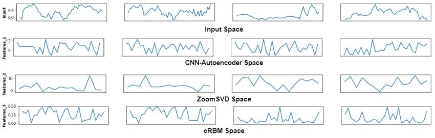
deviate from their true value based on actual fundamentals          •  OHCL Data space is highly dimensional and, as such,
of the asset. Many other factors like economic conditions,             models that try to extract relevant patterns in the raw
correlation to market, etc have an adverse effect on the prices        price data can suffer from the so-called curse of dimen-
but due to limited data and model complexity, they cannot              sionality [26]. We will explore the potential of LFSS
be incorporated in modelling phase.                                    module to extract relevant features from the dynamic
   In this paper, we propose a model-free Deep RL agent                asset price information in a lower dimensional feature
with a modified state space function over the previous works           space. This latent space can hypothetically incorporate
which filters the fluctuations in asset price and derives a            features such as economic conditions or asset funda-
compressed time-series representation containing relevant              mentals.
information for modelling. We introduce the Latent Feature           Rest of the framework is roughly similar to [1] in terms of
State Space Module(LFSS) as a state space to our deep             action space, reward function, etc. We use deep deterministic
RL architecture. This gives a compressed latent state space       policy gradients (DDPG) algorithm [27] as our RL Model
representation of filtered time series in our trading agent. It   with convolutional neural network(CNN) as deep learning
consists of 2 units:                                              architecture for prediction framework.
   • Filtering Unit                                                  Our dataset was stocks constituting S&P 500 with data
   • Latent Feature Extractor Unit                                from 2007-2015 considered for training data and 2016-2019
The filtering unit first takes the raw, unfiltered signal from    used for testing. We design a new benchmark based on
asset prices and outputs a filtered signal using Kalman Filter    technical indicator Stochastic Kd-Index and Mean-Variance
as described in [22]. After the filtered signal is obtained the   model which is a variation of equal-weighted portfolio
Latent Feature Extractor Unit extracts a lower dimensional        benchmark and performs much better than the same. This
latent feature space using 3 models proposed by us:               benchmark is based on the works in [28].
                                                                     To the best of our knowledge, this is the first of many work
   • Autoencoders
                                                                  that leverages the use of latent features as state space, and
   • ZoomSVD
                                                                  further integrates with already known deep RL Framework
   • Restricted Boltzmann Machine
                                                                  in portfolio optimization domain. The main aim of our work
All these 3 models are applied independently and their            is to investigate the effectiveness of Latent Feature State
performance is compared to judge which is the most suitable       Space(LFSS) module added to our RL agent, on the process
to get a compressed latent feature space of the price signal.     of portfolio optimization to get improved result over existing
Autoencoders and Restricted Boltzmann Machine are self-           deep RL framework.
supervised deep learning architecture that are widely used in
dimensionality reduction [23,24] to learn a lower dimension       A. Related Work
representation for an input space, by training the network           With the increased complexity of deep RL models, their
to ignore input noise. Svd(Singular Value Decomposition)          application in Portfolio Optimization has increased widely
is a matrix factorization procedure used widely in machine        over the past years. As we discussed in the last section,
learning and signal processing to get a linear compressed rep-    [15,16,17,18] were one of the breakthrough papers in this
resentation of a time series. We employ ZoomSvd procedure         domain. Our work borrowed many methods from [15,16],
which is a fast and memory efficient method for extracting        which had the advantage of using continuous action space.
SVD in an arbitrary query time range proposed recently in         They used state of the art RL algorithms like DQN, DDPG,
[25].                                                             PPO, etc for various markets. [20] makes a comparison of
   Asset price data are usually processed in OHLC(open,           model-based RL agent and model-free deep RL agent, thus
high, low, close) form and RL state space are built upon the      showing dominance and robustness of model-free Approach.
same. In deep-RL models used in [15,16,20,21,9], returns or       [15] showed CNN architecture performed much better than
price ratio(eg High/close) are used in unprocessed form as        LSTM networks for the task of dynamic optimization of
state space with a backward time step which is the hypothesis     cryptocurrency portfolios, even though LSTM is more ben-
that how much the portfolio weights are determined by the         eficial for time-series data. [9] used a modified reward
assets previous prices. Although most of the RL agents            function that prevented large portfolio weights in a single
applied in research use OHLC State Space, there are still         asset.
several challenges that LFSS Module solves:                          [26,29] were the first to use the concept of an added
   • Financial Data is considered very noisy with distorted       module for improved performance to already existing ar-
      observations due to turbulences caused by the informa-      chitectures. [29] added a State Augmented Reinforcement
      tion published daily along with those sudden market be-     Learning(SARL) module to augment the asset information
      haviours that change asset prices. These intraday noises    which leveraged the power of Natural Language Process-
      are not the actual representative of the asset price and    ing(NLP) for price movement prediction. They used financial
      the real underlying state based on actual fundamentals      news data to represent the external information to be encoded
      of the asset are corrupted by noise. Filtering techniques   and augmented to the final state. [26] used combination
      help approximate the real state from noisy state and        of three modules infused prediction module(IPM), a gen-
      help’s improve quality of data.                             erative adversarial data augmentation module (DAM) and a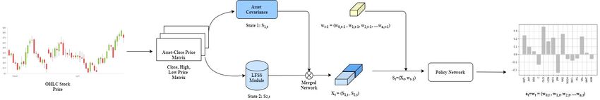
behaviour cloning module (BCM). IPM forecast the future
price movements of each asset, using historical data . DAM
solves the problem of availability of large financial datasets
by increasing the dataset size by making use of GANs and
BCM uses a greedy strategy to reduce volatility in changes
in portfolio weight’s hence reducing transaction cost[26].
                         II. BACKGROUND
A. Portfolio Optimization
   A portfolio is a collection of multiple financial assets, and                       Fig. 1.   Reinforcement Learning Setting [30]
is characterized by its:
   • Component: n assets that comprise it. In our case n =
     15                                                                       A MDP is defined as a 5-tuple (S, A, P, r, γ) described
                                 th                                         below with t being time horizon over portfolio period-
   • Portfolio vector, wt : the i   index illustrates the propor-
     tion of the funds allocated to the ith asset
                                                                                      S
                                                                              • S =     t St is a collection of finite dimensional contin-
                 wt = [w1,t , w2,t , w3,t , ...wn,t ] ∈ Rn                      uous Sstate space of the RL model.
                                                                              • A =      t At is the finite dimensional continuous action
     For w1,t < 0 for any n, implies short selling is allowed.                  space as we consider the market environment as an
We add a risk-free asset to our portfolio for the case if all                   infinite Markov Decision Process (IMDP).
the wealth is to be allocated to a risk-free asset. The weight                • P : S × A × S → [0, 1] is the state transition probability
vector gets modified to                                                         function
                                                                              • r : S × A → R is the instant or the expected instant
               wt = [w0,t , w1,t , w2,t , w3,t , ...wn,t ]           (1)
                                                                                reward at each time index obtained for taking an action
The closing price is defined as vi,t for asset i at time t. The                 in a particular state.
price vector vt = [v0,t , v1,t , v2,t , v3,t , ...vn,t ], consists of the     • γ ∈ (0, 1] is a discount factor. When γ=1 a reward
market prices of the n assets, taken as the closing price of                    maintains its full value at each future time index inde-
the day in this case and constant price of risk-free asset v0,t .               pendent of the relative time from present time step. As γ
Similarly, vthi and vtlo denote the highest prices and the low-                 decreases, the effect of reward in the future is declined
est price vector at time step t, respectively. Over time, asset                 exponentially by γ
price’s change, therefore we denote yt as the relative price
                              v1,t+1 v2,t+1 v3,t+1             vn,t+1 T
vector equal to vt+1
                  vt = (1, v1,t , v2,t , v3,t , .... vn,t ) .               C. Policy Function
   To reduce risk, portfolios with many assets are preferable
over holding single assets. We assume readers have knowl-                      Policy function(π) indicate the behaviour of a RL agent
edge of important concepts of portfolio namely portfolio                    in a given state. π is a “state to action” mapping function,
value, asset returns, portfolio variance, Sharpe ratio, mean-               π : S → A. A policy is either Deterministic At+1 = π(St )
variance model, etc as we will not go in detail of these topics.            or Stochastic: π(S|α). We deal with the mapping to be
These topics are well described in thesis reports [20,9].                   deterministic. Since we are dealing with the case of infinite
                                                                            Markov decision process (IMDP), the policy is modelled
B. Deep RL Model as a Markov Desicion Process                               as a parameterized function with respect to parameter θ
   We briefly review the concepts of DRL and introduce the                  and policy mapping becomes At = πθ (St ). Policy function
mathematics of the RL agent. Reinforcement learning is a                    parameterized with θ is determined solved by using DRL
self-learning method, in which the agent interacts with the                 models like DDPG, DQN, etc which derived from concepts
environment with no defined model and less prior informa-                   of Q-Learning described in the next subsection.
tion, learning from the environment by exploration while at
the same time, optimally updating its strategy to maximize a                D. Q-Learning
performance metric. RL consist of an agent that receives the
                                                                              Q-learning is an approach in reinforcement learning which
controlled state of the system and a reward associated with
                                                                            helps in learning optimal policy function, using the concept
the last state transition. It then calculates an action which
                                                                            of Q-value function. Q-value function is defined as the
is sent back to the system. In response, the system makes a
                                                                            expected total reward when executing action A in state S
transition to a new state and the cycle is repeated as described
                                                                            and henceforth follow a policy π for future time steps.
in fig 1.
   The goal is to learn a set of actions taken for each state                                Qπ (St , At ) = Eπ (rt |St , At )          (2)
(policy) so as to maximize the cumulative reward in dynamic
environment which in our case is the market. RL is mod-                     Since we are using a deterministic policy approach, we can
elled on the concepts of Markov Decision Process(MDP), a                    simplify the Q-function using Bellman Equation as:
stochastic model in discrete time for decision making [9].
They work on the principle of Markov chain.                                   Qπ (St , At ) = Eπ (Rt+1 + γQπ (St+1 , At+1 )|St , At )   (3)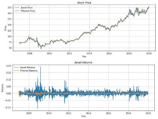
The optimal policy for Qπ is the one which gives maximum            The filtering unit uses Kalman Filter to obtain a linear
Q-function over all policies:                                     hidden state of the returns with the noise being considered
                                                                  Gaussian. The Latent Feature Extractor Unit compares 3
                 π(S) = argmaxQπ (S, A)                     (4)   models Autoencoders, ZoomSVD and RBM, each being used
To speed up the convergence to the optimal policy, concept of     independently with the filtering unit to extract latent feature
replay buffer is used and a target network is used to move        space which is the state space of our deep RL architecture.
the relatively unstable problem of learning the Q function        LFSS module structure can be visualized from figure 2.
closer to the case of supervised learning[16].                    A. Kalman Filter
E. Deep Deterministic Policy Gradient(DDPG)                           Is an algorithm built on the framework of recursive
   DDPG is a model-free algorithm combining Deep Q-               Bayesian estimation, that given a series of temporal mea-
Network (DQN) with Deep Policy Gradient (DPG). DQN                surements containing statistical noise, outputs state estimates
(Deep Q-Network) stabilizes Q-function learning by replay         of hidden underlying states that tend to be more accurate
buffer and the frozen target network [9]. In case of DPG, the     representation of underlying process than those based on
deterministic target policy function is constructed by a deep     an observed measurement [31]. Theory of Bayesian filtering
learning model and the optimal policy is reached by using         is based on hidden Markov model. Kalman Filter assumes
gradient descent algorithm. The action is deterministically       linear modelling and gaussian error (Eq. 6,7). Kalman Filter
outputted by the policy network from the given state. DDPG        is a class of Linear-Quadratic Gaussian Estimator(LQG)
works on actor-critic framework, where the actor network          which have closed-form solution as compared to other
which outputs continuous action, and then the actor per-          filtering methods having approximate solutions(eg Particle
formance is improved according to critic framework which          Filtering)[32]. We used Kalman Filter to clean our return
consist of an appropriate objective function.                     time-series of any Gaussian noise present due to market
   The Preturns from the agent at a time step t is defined as     dynamics. The advantages of Kalman Filter are:
          ∞     k−t
rt =                                                                  • Gives simple but effective state estimates[18] which is
          k=t γ     r(Sk , Ak ) where r is reward function, γ
is the discount factor and return rt is defined as the total            computationally inexpensive
discounted reward from time step t to final time period[15].          • Market’s are highly fluctuating and non-stationary, but
The performance metric of πθ for time interval [0, tf inal] is          the Kalman Filter gives optimal results despite being a
defined as the corresponding reward function:                           LQG estimator.
                                                                      • It is dynamic and works sequentially in real time,
                 J[0,tf inal ] (πθ ) = E(r, Sπθ )                       making predictions only using current measurement
                          T
                          X                                 (5)         and previously estimated state on predefined model
                      =         γ t r(St , πθ (St ))                    dynamics.
                          t=1
                                                                  Though markets may not always be modelled in linear fash-
   The network is assigned random weights initially. With         ion and noises may not be Gaussian, Kalman filter is widely
the gradient descent algorithm (Eq 6) weights are constantly      used and various experiments have proved to be effective
updated to give the best expected performance metric.             for state estimation [31,22]. The mathematical explanation
                 θ ← θ + λ∇θ J[0,tf inal ] (πθ )            (6)   of the filter is given from eq 7-15 [22].

λ is the learning rate. For the portfolio optimization task, we                xt+1 = Ft xt + wt , wt ∼ N (0, Q)              (7)
modify our reward function to be similar to that described                       yt = Gt xt + vt , vt ∼ N (0, R)              (8)
in [15] and we shall describe it in section IV. For training
methodology also we borrow the works of [15] as we use the        where xt and yt are the state estimate and measurements at
concepts of Portfolio Vector Memory(PVM) and stochastic           time index t respectively. Ft is the state transition matrix,
batch optimization. We have only worked with and described        Gt is measurement function. White noises wt (state noise)
in brief DDPG algorithm but other algorithms like Proximal        and vt (process noise) are independent, normally distributed
Policy Optimization(PPO) are widely used.                         with zero mean and constant covariance matrices Q and R
                                                                  respectively.
      III. L ATENT F EATURE S TATE S PACE M ODULE
   Price and returns are usually derived from Open, High,                       xM L           ML
                                                                                 t+1|t+1 = Ft xt|t + Kt+1 εt+1                (9)
Low, Close(OHLC) data. These are unprocessed and contain
                                                                                     εt+1 = yt+1 − Gt xM L
                                                                                                       t+1|t                (10)
high level of noise. Using OHLC data based state space
[15,16,20,21,9] also leads to high dimensionality and the use               Kt+1 = Pt+1|t GTt [Gt Pt+1|t GTt + R]−1         (11)
of extra irrelevant data. LFSS module helps in tackling such
problems by using a filtering unit to reduce noise in the data                       Pt+1|t = Ft Pt|t FtT + Q               (12)
and a Latent Feature Extractor Unit which helps in obtaining                     Pt+1|t+1 = [I − Kt+1 G]Pt+1|t              (13)
a set of compressed latent features which represent the asset-
prices in a more suitable and relevant form.                                               xM  L
                                                                                            0|0 = µ0                        (14)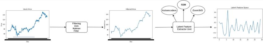
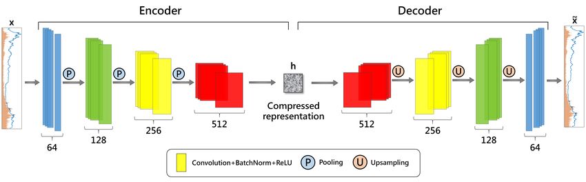
Fig. 2. LFSS Module Structure: (i) The stock price series is passed through a filtering layer which uses Kalman Filter to clean the signal of any Gaussian
noise. (ii) The filtered signal is passed through a Latent Feature Extractor Unit which consists of one of 3 feature extractor methods a) Autoencoders b)
ZoomSVD c) RBM, each applied individually and independently to obtain a lower dimensional signal

                               P0|0 = P0                             (15)      output similar to the input. The mean squared norm loss
                                                                               is used(equation 18,19) as loss function L.
Eq 9-15 give the closed-form solution of Kalman filter using
maximum likelihood estimation(ML). [32] gives a detailed                                     φ, Ω = argminφ,Ω kX − (φ ◦ Ω)Xk2                       (18)
derivation of closed-form solution using ML and Maximum
a posteriori (MAP) estimate. εt is the error estimate defined                                             L = kX − X 0 k2                           (19)
in Eq-10 and Kt is called the Kalman gain and defined in                         For our methodology we compare and select the most
Eq-11. Eq 14-15 gives the initial state assumption of the                      suitable of CNN autoencoder(fig 3), LSTM autoencoders and
process. In the experiment section, we use the Kalman filter                   DNN autoencoders.
for our asset price signal and input the filtered signal to the
Latent Feature Extractor Unit of LFSS module.
B. Autoencoders
   Its a state of the art model from non-linear feature extrac-
tion of time series leveraging the use of deep learning. An
autoencoder is a neural network architecture in which the
output data is the same as input data during training, thus
learns a compact representation of the input, with no need
for labels [23]. Since no output exists i.e. requires no human
intervention such as data labelling it is a domain of self-
supervised learning [33]. The architecture of an autoencoder
                                                                               Fig. 3.     Convolutional-Autoencoder Explained- (i) First the encoder
uses two parts in this transformation[34]                                      consisting of Convolution and Pooling Layer, compresses the input time
   • Encoder- by which it transforms its high dimensional                      series to lower dimension. (ii) Decoder reconstructs the input space using
      inputs into a lower dimension space while keeping the                    upsampling and Convolution layer [35]
      most important features
                                 φ(X) → E                            (16)      C. ZoomSVD: Fast and Memory Efficient Method for Ex-
                                                                               tracting SVD of a time series in Arbitrary Time Range-
   •   Decoder- which tries to reconstruct the original input
       from the output of the encoder                                             Based on the works in [25], this method proposes an
                                                                               efficient way of calculating the Singular Value Decompo-
                                 Ω(E) → X                            (17)      sition(SVD) of time series in any particular range. The SVD
The output of the encoder is the latent-space representation                   for a matrix is as defined in Eq 20.
which is of interest to us. It is a compressed form of                                                      A = U ΣV T                              (20)
the input data in which the most influential and significant
features are kept. The key objective of autoencoders is to                        If A has dimensions M × N (for time series case, M is
not directly replicate the input into the output [34] i.e learn                the length of time period and N is the number of assets)
an identity function. The output is the original input with                    then for case of compact-SVD(form of SVD used) U is
certain information loss. Encoder should map the input to a                    M × R and V is N × R orthogonal matrices such that
lower dimension than input as a larger dimension may lead                      U U T = IRxR and V V T = IRxR and R ≤ min[M, N ] is
to learning an identity function.                                              the rank of A. U and V are called left-singular vectors and
   The encoder-decoder weights are learnt using backprop-                      right-singular vectors of A. Σ=diag(d1 , d2 , d3 , ...dR ) is a
agation similar to supervised learning approach but with                       square diagonal of size R × R with d1 ≥ d2 ≥ d3 , ... ≥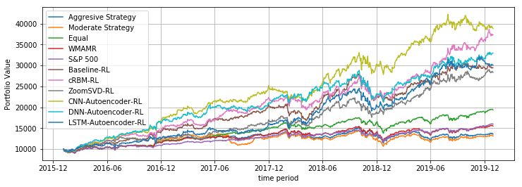
Fig. 4. ZoomSVD representation from [13]- (i) In the Storage-Phase the original asset-price series matrix is divided in blocks and compressed to lower
dimensional SVD form using incremental-SVD. (ii) In Query-Phase, SVD in reconstructed from the compressed block structure in storage phase, for a
particular time-query [ti , tf ] using Partial-SVD and Stitched-SVD [25]

dR ≥ 0 and are called singular values of A. For time                         other methods[25]. For the case of portfolio optimization
series data, A = [A1 ; A2 ; A3 ; ....AN ] where Ai is column                 problem, we use ΣV T as our state space. The right singular
matrix of time series values within a range and A is the                     vector represents the characteristics of the time series matrix
vertical concatenation of each Ai . The SVD of a matrix can                  A and the singular value’s represents the strength of the
be calculated by many numerical methods known in linear                      corresponding right singular vector [37]. U is not used
algebra. Some of the methods are described in [36].                          because of high dimensionality due to the large time horizon
   SVD is a widely used numerical method to discover                         required by the RL agent.
hidden/latent factors in multiple time series data [25], and
in many other applications including principal component                     D. Restricted Boltzmann machine: Probabilistic representa-
analysis, signal processing, etc. While autoencoders extract                 tion of the training data
non-linear features from high dimensional time series, SVD                      Restricted Boltzmann machine is based on the works of
is much simpler and finds linear patterns in the dimension                   [38], and has similar utility to the above mentioned methods
of time series thus leading to less overfitting in many cases.               in fields like collaborative filtering, dimensionality reduction,
Zoom-SVD incrementally and sequentially compresses time                      etc. A restricted Boltzmann machine (RBM) is a form of
series matrix in a block by block approach to reduce the                     artificial neural network that trains to learn a probability
space cost in storage phase, and for a given time range query                distribution over its set of inputs and is made up of two
computes singular value decomposition (SVD) in query                         layers: the visible and the hidden layer. The visible layer
phase by methodologically stitching stored SVD results [25].                 represents the input data and the hidden layer tries to learn
ZoomSVD is divided in 2 phases-                                              feature-space from the visible layer aiming to represent a
   • Storage Phase of Zoom-SVD                                               probabilistic distribution of the data [39]. Its an energy-
        – Block Matrix
        – Incremental SVD
   • Query Phase of Zoom-SVD
        – Partial-SVD
        – Stitched-SVD
   Figure 4 explains the original structure proposed in [25].
In storage phase, time series matrix A is divided into blocks
of size b decided beforehand. SVD of each block is computed
sequentially and stored discarding original matrix A. In the
query phase, an input query range [ti ,tf ] is passed and
using the block structure the blocks containing the range are
                                                                             Fig. 5. RBM structure consisting of 3 visible units and 2 hidden units with
considered. From the selected blocks, initial and final blocks               weights w and bias a,b, forming a bipartite graph structure [39]
contain partial time ranges. Partial-SVD is used to compute
SVD for initial and final blocks and is merged with SVD of                   based model implying that the probability distribution over
complete blocks using Stitched-SVD to give final SVD for                     the variables v(visible layer) and h(hidden layer) is defined
query range [ti ,tf ]. Further explanation of the mathematical               by an entropy function in vector form(Eq 21).
formulation of the storage and query phase are described in
[25].                                                                                        E(v, h) = −hT W v − aT v − bT h                      (21)
   ZoomSVD solves the problem of expensive computational
cost and large storage space in some cases. In comparison to                 where W is the weights, a and b are bias added.
traditional SVD methods, ZoomSVD computes time range                            RBM’s have been mainly used for binary data, but there
queries up to 15x faster and requires 15x less space than                    are some works [39,40] which present new variations for
dealing with continuous data using a modification to RBM          C. Action Space
called Gaussian-Bernoulli RBM (GBRBM). We further add
                                                                    To solve the dynamic asset allocation task, the trading
extension of RBM, conditional RBM(cRBM) [24,41]. The
                                                                  agent must at every time step t be able to regulate the
cRBM has auto-regressive weights that model short-term
                                                                  portfolio weights wt . The action at at the time t is the
temporal dependencies and hidden layer unit that model
                                                                  portfolio vector wt at the time t:
long-term temporal structure in time-series data [24]. A
cRBM is similar to RBM’s except that the bias vector for                        at ≡ wt = [w1,t , w2,t , w3,t , ...wn,t ]                   (22)
both layers is dynamic and depends on previous visible layers
[24]. We will further refer to RBM as cRBM in the paper.          The action space A is thus a subset of the continuous Rn
  Restricted Boltzmann machines uses contrastive diver-           real n-dimensional space:
gence (CD) algorithm to train the network to maximize input                                           n
probability. We refer to [39,24] for further explanation of                                           X
                                                                                 at ∈ A ⊆ R n ,             ai,t = 1, ∀t ≥ 0                (23)
mathematics of RBM’s and cRBM’s.
                                                                                                      i=1

                                                                  The action space is continuous (infinite) and therefore con-
               IV. P ROBLEM F ORMULATION
                                                                  sider the stock market as an infinite decision-making process
   In the previous section, we had described RL agent formu-      for MDP(IMDP) [9].
lation in terms of Markov decision process defined using 5
tuple (S, A, P, r, γ). In this section we describe each element   D. OHLC Based State Space
of tuple with respect to our portfolio optimization problem          Before we describe the novel state space structure used by
along with the dataset used and the network architecture used     our RL agent, we describe the state space based on OHLC
as our policy network.                                            data being used in previous works. In later sections, we
                                                                  showcase the superior performance of our novel state space
A. Market Assumptions                                             based RL agent.
                                                                     Using the data in OHLC form, [15] considered closing,
   In a market environment, some assumptions are considered       high and low prices to form input tensor for state space of RL
close to reality if the trading volume of the asset in a market   agent. The dimension of input is (n,m,3)(some works may
is high. Since we are dealing with stocks from S&P 500            define dimensions in (3,m,n) form), where n is the number
the trading volume is significantly high(high liquidity) to       of assets, m is the window size and 3 denotes the number of
consider 2 major assumptions:                                     price forms. All the prices are normalized by closing price
  •   Zero Slippage- Due to high liquidity, each trade can be     vt at time t. The individual price tensors can be written as:
      carried out immediately at the last price when an order
      is placed
  •   Zero Market Impact- The wealth invested by our agent         Vt = [vt−m+1 vt |vt−m+2 vt |vt−m+3 vt |..|vt vt ] (24)
      insignificant to make an influence on the market
                                                                    (hi)      (hi)             (hi)              (hi)                (hi)
                                                                  Vt       = [vt−m+1     vt |vt−m+2          vt |vt−m+3      vt |..|vt       vt ]
                                                                                                                                            (25)
B. Dataset                                                          (lo)      (lo)            (lo)               (lo)                (lo)
                                                                  Vt       = [vt−m+1     vt |vt−m+2          vt |vt−m+3      vt |..|vt
                                                                                                                           vt ]
   The S&P 500 is an American stock market index based                                                                   (26)
on the market capitalization of 500 large companies. There                      (hi) (lo)
                                                                    Where vt , vt , vt represents the asset close, high and
are about 500 tradable stocks constituting S&P 500 index          low prices at time t,      represents element-wise division
however, we will only be using a subset of 15 randomly            operator and | represents horizontal concatenation. Vt is
selected stocks for our portfolio. The stocks were- Apple,        defined individually for each asset as
Amex, Citi bank, Gilead, Berkshire Hathaway, Honeywell,
Intuit, JPMC, Nike, NVDIA, Oracle, Procter & Gamble,                                 Vt = [V1,t ; V2,t ; V3,t ; ..; Vn,t ]                  (27)
Walmart, Exxon Mobile and United Airlines Holdings. We
took stocks from various sectors to diversify our portfolio.      where Vi,t is close price vector for asset i and ; represents
                                                                                                                   (hi)       (lo)
   We took the data from January 2007 to December 2019,           vertical concatenation. Similar is defined for Vt     and Vt .
that made up a dataset of total size of 3271 rows. 70 %           Xt is the final state space formed by stacking layers Vt ,
                                                                    (hi)    (lo)
(2266 prices, 2007-2015) of data was considered as training       Vt , Vt        as seen in figure 6.
set and 30% as testing set(1005 prices, 2016-2019). This             In order to incorporate constraints like transaction cost,
large span of time subjects our RL agent to different types of    the state space Xt at time t is combined with previous
market scenarios and learns optimal strategies in both bearish    time step portfolio weight wt−1 to form final state space
and bullish market. For our risk-free asset to invest in case     St = (Xt , wt−1 ). The addition of wt−1 to state space has
investing in stocks is risky, we use a bond with a constant       been widely used in other works [15,16,20,21,9] to model
return of 0.05 % annually.                                        transaction cost of portfolio.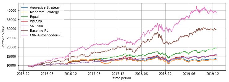
account practical constraints, its near-optimality with respect
                                                                      to portfolio performance and should be easily differentiable.
                                                                      Applying the reward function used in [15] satisfying all of
                                                                      the above conditions, the reward function at time t is :
                                                                                                                n
                                                                                                                X
                                                                            rt = r(st , at ) = ln(at · yt − c         |ai,t − wi,t |)   (28)
                                                                                                                i=1

                                                                      As explained by Eq 4, the performance objective function is
                                                                      defined as:
                                                                                                          T
                                                                                                       1 X t
                                                                                 J[0,tf inal ] (πθ ) =       γ r(St , πθ (St ))         (29)
                                                                                                       T t=1

   Fig. 6.   OHLC state space in 3-dimensional input structure [15]   where γ is discount factor and r(St , πθ (St )) is the immediate
                                                                      reward at time t with policy function πθ (St ). We modify Eq
                                                                      5 by dividing it by T which is used to normalize the objective
E. LFSS Module Based State Space                                      function for time periods of different length. The main
   LFSS module based state space consisted of two asset               objective involves maximizing performance objective based
features that were processed individually through different           on policy function πθ (St ) parametrized by θ. The network is
neural networks and merged after processing. The state space          assigned random weights initially. With the gradient descent
considered was based on time-series features of asset returns         algorithm(Eq 6) weights are constantly updated to give the
for 15 assets in our portfolio. The asset feature extracted           best expected performance metric, based on the actor-critic
were-                                                                 network.
   • Covariance Matrix- the symmetric matrix for 15 assets                              θ ← θ + λ∇θ J[0,tf inal ] (πθ )                 (30)
     was calculated. This part of the state space signifies the
     risk/volatility and dependency part of each asset with           G. Input Dimensions
     one another. 3 matrix for close, high and low prices
                                                                         LFSS Module used considered two deep learning tech-
     were computed giving a 15 × 15 × 3inputmatrix.
                                                                      niques Autoencoders and cRBM for feature extraction of
   • LFSS Module Features- We described Filtering unit to
                                                                      time-series. While ZoomSVD has a static method for rep-
     clean the time series followed by 3 different methods
                                                                      resentation and we kept fixed size of cRBM structure, we
     Autoencoder, ZoomSVD, RBM in Latent Feature Ex-
                                                                      compared different network topology’s used for training
     tractor Unit to extract latent features. Close, high and
                                                                      autoencoders. 3 types of neural networks- Convolutional
     low prices were individually processed by LFSS module
                                                                      Neural Network(CNN), Long-Short Term Memory(LSTM)
     to form 3 dimensional structure similar to figure 6 but
                                                                      and Deep Neural Network(DNN) were compared, with the
     in a lower-dimensional feature space.
                                                                      corresponding results shown in the experiments section. Our
   Similar to technique mentioned in last sub-section, previ-         input signal consisted of considering window-size of 60 days
ous time step portfolio weight wt−1 is added to form final            or roughly 2 months price data, giving sufficient information
state space St = (Xt , wt−1 ), where Xt is merged network             at each time step t. The window-size is adjustable as this
result.                                                               value is experiment based and there is no theoretical backing
F. Reward Function                                                    of choosing 60 days window. Since we are using 15 assets
                                                                      in our portfolio the state space concept used by [15] based
   A key challenge in portfolio optimization is controlling           on OHLC data, has input size of 15×60×3, where 60 is the
transaction costs(brokers’ commissions, tax, spreads, etc)            window size, 15 is the number of assets and 3 representing
which is a practical constraint to consider to not get bias           3 prices close, high and low. We added the asset covariance
in estimating returns. Whenever the portfolio is re-balanced,         matrix in our state space, along with LFSS module features,
the corresponding transaction cost is deducted from the               which has dimensions of 15×15×1. The LFSS module
portfolio return. Many trading strategies work on the basic           feature space for individual methods had dimensions as
assumption on neglecting transaction cost, hence are not              follows-
suitable for real-life trading and only obtain optimality using
greedy algorithm(e.g allocating all the wealth into the asset           •   Autoencoder - 15×30×3
which has the most promising expected growth rate) without              •   ZoomSVD - 15×15×3
considering transaction cost. Going by the rule of thumb                •   cRBM - 15×30×3
the transaction commission is taken as 0.2% for every buy             Autoencoders and cRBM provide flexibility of reducing the
and sell re-balancing activity i.e c = cb = cs = 0.2. We              original price input into variable-sized feature space, while
have to consider such a reward function which takes into              ZoomSVD has drawback of fixed-sized mapping.
Fig. 7. The framework of our proposed LFSS Module based RL Agent. Asset prices are structured in 3-dimensional close, high and low price and then
the state space S1,t and S2,t are extracted from state-covariance and LFSS module, and a combined state Xt is formed from a merged Neural Network.
Combined with previous timestep action space at−1 , a new portfolio vector is formed for time t through the policy network

H. Network Architecture                                                      •   S&P 500 - the stock-market index which depicts the
                                                                                 macro-level movement of the market as a whole.
   Our Deterministic target policy function is constructed
                                                                             •   OHLC State-Space Rl Agen(Baseline-RL) - uses unpro-
by a neural network architecture used by the agent. Sev-
                                                                                 cessed asset prices as state space and trains the agent
eral variations of architecture are used for building policy
                                                                                 with a CNN approximated policy function. It is the most
function revolving around CNN, LSTM, etc. To establish
                                                                                 widely used RL agent structure for dynamic portfolio
the performance of Latent Feature State Space compared to
                                                                                 optimization.
OHLC state space, we work with single model architecture
                                                                             •   Weighted Moving Average Mean Reversion(WMAMR)
for better judgement of performance of various state-spaces.
                                                                                 - is a method which captures information from past pe-
Considering the results in [15,20,21], CNN based network
                                                                                 riod price relatives using moving averaged loss function
outperformed RNN and LSTM for approximating policy
                                                                                 to achieve an optimal portfolio.
function, due to its ease in handling large amounts of
                                                                             •   Integrated Mean-Variance Kd-Index Baseline(IMVK)-
multidimensional data, though this result is empirical as
                                                                                 derived from [28], this works on selecting a subset of
sequential neural network like RNN and LSTM should model
                                                                                 given portfolio asset based on technical-indicator Kd-
price data better than CNN[15].
                                                                                 Index and mean-variance model[6], and allocates equal-
   Motivated by [15] we used similar techniques, namely                          weights to the subset at each time-step. For calculating
Identical Independent Evaluators(IIE) and Portfolio-Vector                       Kd-Index first a raw stochastic value(RSV) is calculated
Memory(PVM) for our trading agent. In IIE, the policy                            as follows:
network propagates independently for the n+1 assets with
common network parameters shared between each flow. The                                                    (vt − vmin )
scalar output of each identical stream is normalized by                                       RSVt =                    × 100                (31)
                                                                                                         (vmax − vmin )
the softmax layer and compressed into a weight vector as
the next period’s action. PVM allows simultaneous mini-                          vt , vmax , vmin represent the closing price at time t,
batch training of the network, enormously improving training                     highest closing price and lowest closing price, respec-
efficiency [15].                                                                 tively. Kd-Index is computed as:
   Our state space consists of 3 parts- LFSS Module Features,
covariance matrix and the portfolio vector from the previous                                                     1          2
                                                                                               Kt = RSVt ×         + Kt−1 ×                  (32)
rebalancing step(wt−1 ). LFSS and covariance matrix were                                                         3          3
individually processed through CNN architecture, and con-
catenated together into a single vector Xt after individual                                                     1          2
                                                                                                 Dt = Kt ×        + Dt−1 ×                   (33)
layers of processing. The previous actions, wt−1 , is concate-                                                  3          3
nated to this vector to form final stage state St = (Xt , wt−1 ).
This is passed through a deep neural network, with IIE and                       where K1 = D1 = 50. Whenever Kt−1 ≤ Dt−1
PVM setup, to output portfolio vector wt with the training                       and Kt > Dt , a buy signal is created. Two strategies,
process as described in the previous subsection. The basic                       Moderate and aggressive, are formed upon Kd-Index.
layout of our RL agent is as given in figure 7.                                  Moderate strategy works on selecting an asset only if
                                                                                 Mean-Variance model weights for the asset is positive
                                                                                 and Kd-Index indicated a buy signal at that time-step.
I. Benchmarks
                                                                                 Aggressive strategy selects an asset only based on Kd-
  •   Equal Weight Baseline(EW) - is a trivial baseline which                    Index indicating a buy signal. Equal distribution of
      assigns equal weight to all assets in the portfolio.                       wealth is done on the subset.
Autoencoder Training Summary
V. E XPERIMENTAL R ESULTS LSTM CNN DNN
Training set Mse 0.0610 0.0567 0.0593
A. Filtering Unit Test set Mse 0.0592 0.0531 0.0554
As described before, LFSS Module has an added Filtering Epochs 125 100 100
Unit consisting of a Kalman Filter to filter out noise from
TABLE I
price data of each asset. Since deep learning model are
sensitive to the quality of data used, many complex deep
learning models may overfit the data, learning noise in the
data as well, thus not generalizing well to different datasets. cRBM Space- We use a cRBM network stacked of 2
Each of the asset prices was filtered before passing to the layers(1 visible layer, 1 hidden layer). Visible unit corre-
Latent Feature Extractor Unit. sponding to the asset price window(60) and 30 neurons in
the hidden layer for extracted feature space.
Fig. 8. Filtering Unit: Filtered Berkshire Hathaway Price and Returns
Signal
Fig. 9. Extracted Features from Input Price Window. Feature-1, 2, 3
corresponds to CNN-Autoencoder, ZoomSVD and cRBM extracted space,
respectively
B. Latent Feature Extractor Unit
Autoencoder Space- We build a time-series price encoder C. Training Step
based on 3 encoder-decoder models- LSTM, CNN and DNN For each individual RL agent, number of episodes were
based autoencoders. We used a window size of 60 and the decided on the convergence of percentage-distance from
input consisted of price windows for each asset. To get equal-weighted portfolio returns. A stable learning rate of
better scalability of data, log returns were normalized by the 0.01 of adam optimizer was used, with 32 as batch size. The
min-max scalar. The data was divided into 80-20% training- exploration probability is 20% initially and decreases after
testing dataset. every episode.
The training process summary is as given in table 1,
for both training and testing data. Number of epochs were D. Comparison of LFSS module based RL Agent with
decided on the convergence of mean-squared error of the Baseline-RL agent
autoencoder i.e L = kX − X 0 k2 . After setting up LFSS module and integrating it to policy
network, we backtested the results on given stock portfolio.
ZoomSVD Space- Storage-Phase of ZoomSVD required Table 10 gives comparison summary of different feature
dividing the input price data into blocks, and storing the extraction methods with one another and baseline-RL agent.
initial asset-price matrix in compressed SVD form. The block Initial portfolio investment is 10000$.
parameter b was taken as 60, but is usually decided on As shown in Table 10, adding cRBM and CNN-
storage power of systems for large datasets. SVD of each Autoencoder based LFSS module to the agent leads
block is stored by incremental-SVD. As our time-range query to a significant increase in different performance met-
is passed by our RL agent, the SVD based state-space is ric, while DNN-Autoencoder based LFSS module gives
computed by Partial and stitched-SVD. slightly better performance than baseline-RL. ZoomSVD andPerformance Summary
LSTM-Autoencoder state space performs roughly similar to Portfolio- Annual Annual Sharpe- Sortino-
baseline-RL. Individual performance metric for each asset is Value($) Returns Volatil- Ratio Ratio
described below- ity
Baseline RL 29440 0.486 0.254 1.91 2.12
• Portfolio-Value(PV)- In terms of portfolio value over a DNN- 32960 0.575 0.252 2.28 2.51
span of 4 years on training-set an initial investment of Autoencoder
10000$ reached roughly 39000$ for test-set for CNN- RL
cRBM RL 37368 0.684 0.256 2.67 2.92
Autoencoder and cRBM RL-agent, which performed ZoomSVD 28343 0.458 0.257 1.78 2.03
significantly better than baseline RL-agent. The addi- RL
tion of autoencoder and RBM based LFSS module CNN- 38864 0.722 0.254 2.84 3.04
Autoencoder
models the asset-market environment in a better way RL
than raw price data for the RL-agent. Deep-learning LSTM- 30121 0.503 0.255 1.97 2.13
based feature selection methods could model non-linear Autoencoder
RL
features in asset-price data as compared to linear space
in ZoomSVD. Though cRBM RL agent did not give TABLE II
high returns in the initial years, it had a sharp increase P ERFORMANCE METRIC FOR DIFFERENT RL AGENTS
in portfolio value in later years, performing much better
than other methods during this period.
• Sharpe-Ratio- Most of the models performed similarly
in terms of volatility, with returns varying. There was
no statistically significant difference in volatilities. This • Portfolio-Value- In terms of portfolio value our RL
implies the LFSS module added is in not learning agent and the baseline-RL performs much better than all
anything new to minimize risk in the model. This may the benchmarks used. This shows the superiority of deep
be due to the simplicity of reward function used, and RL based methods for the task of portfolio optimization.
more work will be required to incorporate risk-adjusted For the test set, equal-weighted portfolio gave better
reward to handle volatility, which fits in with DDPG results than all our benchmarks. IMVK based strategies
algorithm. performed poorly on test set, mostly due to high change
• Sortino Ratio- Addition of LFSS module, reduces down-
in weights leading to high transaction cost. If we
side deviation to some extent to the RL agent, but consider the overall time period from 2007-2019 (fig
overall a more effective reward function can minimize 13), IMVK based strategies perform much better than
downward deviation further. equal-weighted portfolio till 2017, followed by a large
drop in portfolio performance.
• Sharpe Ratio- Similar to high returns given by RL
agents, deep RL based approach gave much better
Sharpe Ratio than the benchmarks. Though there was
high difference in volatility, the risk was compensated
by the high returns.
• Sortino Ratio- Similar to Sharpe ratio, RL agents per-
formed much better to all other benchmarks.
Fig. 10. Comparison of various RL agents
E. Performace Measure w.r.t to Benchmarks
We used 5 non-RL based benchmarks for comparison of
our agent with standard portfolio optimization techniques.
The 5 benchmarks used were EW, S&P 500, WMAMR,
IMVK(Moderate and Aggressive Strategy) as explained in
the last section. We compare these benchmarks to one other
Fig. 11. Comparison of RL agent with various benchmarks
and to our RL-agent. The performance summary for all the
methods is as described in table 3.Performance Summary
Baseline- DNN- cRBM ZoomSVD CNN- LSTM- EW Aggressive Moderate S&P WMAMR
RL Autoencoder RL RL Autoencoder Autoencoder Strategy Strategy 500
RL RL RL
Portfolio 29440 32960 37368 28343 38864 30121 19456 13604 13144 15970 15524
Value($)
Annual 0.486 0.575 0.684 0.458 0.722 0.503 0.235 0.0953 0.0785 0.149 0.152
Returns
Annual 0.254 0.252 0.256 0.257 0.254 0.255 0.144 0.162 0.154 0.128 0.144
Volatility
Sharpe 1.91 2.28 2.67 1.78 2.84 1.97 1.63 0.59 0.51 1.16 1.06
Ratio
Sortino 2.12 2.51 2.92 2.03 3.04 2.13 1.84 0.78 0.69 1.37 1.26
Ratio
TABLE III
P ERFORMANCE METRIC FOR ALL THE PROPOSED METHODS
Fig. 12. Backtest Results for all methods proposed Fig. 13. Comparison of Aggressive and Moderate Strategy IMVK with
Equal-Weighted Portfolio
VI. CONCLUSIONS
modelling framework for various different state space with
In this paper, we propose a RL agent for portfolio opti- more sophisticated deep learning models and with the ad-
mization with an added LFSS Module to obtain a novel state vancements in RL algorithms our RL agent can be further
space. We compared the performances of our RL agent with improved upon.
already existing approaches for a portfolio of 15 S&P 500
stocks. Our agent performed much better than baseline-RL VII. F UTURE W ORK
agent and other benchmarks in terms of different metrics like Due to the flexible approach in state space modelling, there
portfolio value, Sharpe Ratio, Sortino Ratio, etc. The main are many ways to improve upon the performance of the RL
catalyst for improvement in returns was due to the addition agent. To improve upon the quality of data through filtering
of LFSS module which consisted of a time series filtering layer, non-linear filters can be applied like EKF, particle
unit and latent feature extractor unit, to get a compressed filter, etc[32], which take into account the non-linearity in
latent feature state space for the policy network. We further the data or use an adaptive filter[452] that at each time
compared different feature space extracting methods like step uses most appropriate filter out of a set of filters. For
autoencoders, ZoomSVD and cRBM. Deep learning based extracting latent features, cRBM can be further extended to
techniques like CNN-Autoencoder and cRBM performed deep belief networks[43], which goes deeper than cRBM and
effectively in obtaining a state-space for our RL agent, is trained using a similar approach . Since RL is highly
that gave high returns, while minimizing risk. Addition- sensitive to the data used, our agent should be trained on
ally, we also introduced a new benchmark based on Kd- more datasets, which are more volatile than American stock
Index technical-indicator, that gave comparable performance exchange data, as this will give a more robust performance.
to equal-weighted portfolio, and can be further used as a Additionally, we can add data augmentation module[26] to
benchmark for more portfolio optimization problems. generate synthetic data, hence exposing the agent to more
The work done in this paper can provide a flexible data. Text data based embedding can also be added to thestate space[29], leveraging the use of NLP techniques. [19] Moody, J. and Saffell, M., Learning to trade via direct reinforce-
In terms of deep RL algorithms, PPO was not used in this ment, IEEE transactions on neural networks, 12 (4):875–889,
2001.
work. Performance of LFSS module with PPO algorithm can [20] Filos A., Reinforcement Learning for Portfolio Management[J].
be further explored. This framework can be integrated with arXiv preprint arXiv:1909.09571, 2019.
appropriate risk-adjusted reward-function that minimizes the [21] J. Kanwar, N., et al, Deep Reinforcement Learning-based Port-
folio Management. Ph.D. Dissertation, 2019.
risk of our asset allocation. [22] Y. Xu and G. Zhang, “Application of kalman filter in the predic-
tion of stock price,” in International Symposium on Knowledge
VIII. ACKNOWLEDGEMENT Acquisition and Modeling (KAM), Atlantis press, pp. 197–198,
This work was supported by Professor Nitin Gupta and 2015.
[23] G.E. Hinton and R.R. Salakhutdinov, Reducing the dimension-
Professor Geetanjali Panda- Department of Mathematics. I ality of data with neural networks. Science, 313(5786):504–507,
would like to thank them for helpful insights on financial 2006.
portfolio optimization, MDP and non-linear optimization, [24] Langkvist, M., Modeling Time-Series with Deep Networks,
Ph.D. Thesis, Orebro University, Orebro, Sweden, 2014.
which was essential in the progress of the project. [25] J.-G. Jang, D. Choi, J. Jung and U. Kang, "Zoom-svd: Fast
and memory efficient method for extracting key patterns in an
R EFERENCES arbitrary time range", CIKM, pp. 1083-1092, 2018.
[1] Y. Feng and D. P. Palomar, “A Signal Processing Perspective [26] Yu, P., Lee, J. S., Kulyatin, I., Shi, Z., and Dasgupta S,
of Financial Engineering”, Foundations and Trends in Signal Model-based deep reinforcement learning for dynamic portfolio
Processing, vol. 9, no. 1-2, pp. 1-231, 2015. optimization. arXiv preprint arXiv:1901.08740, 2019.
[2] M. Japundžić, D. Jočić and I. Pavkov, "Application of stochastic [27] Silver, David, et al., ”Deterministic policy gradient algorithms”,
control theory to the optimal portfolio selection problem," ICML, 2014.
2012 IEEE 10th Jubilee International Symposium on Intelligent [28] Lin JL., Wu CH., Khomnotai L, Integration of Mean–Variance
Systems and Informatics, Subotica, pp. 85-88, 2012. Model and Stochastic Indicator for Portfolio Optimization. In:
[3] Kovalerchuk B., Vityaev E., Data Mining for Financial Ap- Juang J., Chen CY., Yang CF. (eds) Proceedings of the 2nd
plications. In: Maimon O., Rokach L. (eds) Data Mining and International Conference on Intelligent Technologies and En-
Knowledge Discovery Handbook. Springer, Boston, MA, 2005. gineering Systems (ICITES2013), Lecture Notes in Electrical
[4] Heaton, J.; Polson, N.; and Witte, J. H., Deep learning for Engineering, vol 293. Springer, Cham, 2014.
finance: deep portfolios. Applied Stochastic Models in Business [29] Ye, Yunan, Hengzhi Pei, Boxin Wang, Pin-Yu Chen, Yada Zhu,
and Industry 33(1):3–12, 2017. Jun Xiao, and Bo Li, Reinforcement-learning based portfolio
[5] R. Asadi and A. Regan, “A spatial-temporal decomposition management with augmented asset movement prediction states,
based deep neural network for time series forecasting”, arXiv AAAI, 2020.
preprint arXiv:1902.00636, 2019. [30] Sutton, R. and Barto, A. (1998). Reinforcement learning: An
[6] Markowitz, H. M., Portfolio selection: Efficient diversification introduction. Cambridge, MA, MIT Press, 1998.
of investment, 344 p, 1959. [31] James Martin Rankin, Kalman filtering approach to market price
[7] Haugh, M.B., L. Kogan and Z. Wu., Portfolio Optimization with forecasting. PhD thesis, Iowa State University, 1986.
Position Constraints: an Approximate Dynamic Programming [32] Chen, Z., Bayesian filtering: From Kalman filters to particle
Approach. Working paper. Columbia University and MIT, 2006. filters, and beyond. Tech. Rep. McMaster Univ., Canada, 2003.
[8] Cai, Y., K. L. Judd, and R. Xu., Numerical solution of dynamic [33] Vincent, P., Larochelle, H., Lajoie, I., Bengio, Y., Manzagol,
portfolio optimization with transaction costs, NBER Working P.-A. Stacked denoising autoencoders: Learning useful repre-
Paper No. w18709, 2013. sentations in a deep network with a local denoising criterion. J
[9] Antonios Vogiatzis, Reinforcement Learning for Financial Port- Mach Learn Res 11, 3371–3408, 2010.
folio Management- Diploma Thesis, 2019. [34] Nigel Bosch, Unsupervised Deep Autoencoders for Feature Ex-
[10] Kober, J., Bagnell, J. A., Peters, J. Reinforcement learning traction with Educational Data, In Proceedings of the EDM 2017
in robotics: A survey, The International Journal of Robotics Workshops and Tutorials co-located with the 10th International
Research 32, 1238–1274, 2013. Conference on Educational Data Mining, EDM, Urbana, IL,
[11] Y. Zhu, R. Mottaghi, E. Kolve, J. J. Lim, A. Gupta, L. USA, 2017.
FeiFei, and A. Farhadi, Target-driven visual navigation in in- [35] Vladimir Puzyrev. "Deep convolutional autoencoder for cryp-
door scenes using deep reinforcement learning, arXiv preprint tocurrency market analysis," Papers 1910.12281, arXiv.org,
arXiv:1609.05143, 2016. 2019.
[12] Szita I., Reinforcement Learning in Games, In: Wiering M., van [36] Zhang W., Arvanitis A. and Al-Rasheed A., “Singular Value De-
Otterlo M. (eds) Reinforcement Learning. Adaptation, Learning, composition and its numerical computations,” Michigan Tech-
and Optimization, vol 12. Springer, Berlin, Heidelberg, 2012. nological University, Michigan, 2012.
[13] Dixon M.F., Halperin I., Bilokon P., Applications of Reinforce- [37] Hayashi, Isao and Jiang, Yinlai and Wang, Shuoyu, SVD-
ment Learning. In: Machine Learning in Finance. Springer, Based Feature Extraction from Time-Series Motion Data and
Cham, 2020. Its Application to Gesture Recognition, Proceedings of the
[14] J. Ahmet Murat Ozbayoglu, Mehmet Ugur Gudelek, and Omer 8th International Conference on Bioinspired Information and
Berat Sezer, Deep learning for financial applications: A survey. Communications Technologies:386-387, 2014.
working paper, 2019. [38] Salakhutdinov, R., Mnih, A., and Hinton, G. E. (2007), Re-
[15] Jiang, Zhengyao, Dixing Xu, and Jinjun Liang, ”A deep rein- stricted Boltzmann machines for collaborative filtering, In ICML
forcement learning framework for the financial portfolio man- 2007.
agement problem.” arXiv preprint arXiv:1706.10059, 2017. [39] R. Hrasko, A. G. C. Pacheco, and R. A. Krohling, “Time
[16] Liang, Z., Chen, H., et al, Adversarial Deep Reinforcement Series Prediction Using Restricted Boltzmann Machines and
Learning in Portfolio Management. arXiv:1808.09940, 2018. Backpropagation,” Procedia Computer Science, vol. 55, no.
[17] C. [Almahdi and Yang 2017] Almahdi, S., and Yang, S. Y., Itqm, pp. 990–999, 2015.
An adaptive portfolio trading system: A risk-return portfolio [40] Kuremoto T., Kimura S., Kobayashi K., Obayashi M., Time
optimization using recurrent reinforcement learning with ex- Series Forecasting Using Restricted Boltzmann Machine, In:
pected maximum drawdown. Expert, Systems with Applications Huang DS., Gupta P., Zhang X., Premaratne P. (eds) Emerging
87:267–279, 2017. Intelligent Computing Technology and Applications, ICIC 2012,
[18] J. Moody, M. Saffell, Y. Liao. Reinforcement learning for Communications in Computer and Information Science, vol 304.
trading systems and portfolios, In SIGKDD International Con- Springer, Berlin, Heidelberg, 2012.
ference on Knowledge Discovery and Data Mining, pp. 129-140, [41] G. W. Taylor and G. E. Hinton, Factored conditional restricted
1998. Boltzmann machines for modeling motion style, In ICML, 2009.You can also read