WORKING PAPER - DEPARTMENT OF ECONOMICS AND FINANCE SCHOOL OF BUSINESS AND ECONOMICS UNIVERSITY OF CANTERBURY CHRISTCHURCH, NEW ZEALAND

DEPARTMENT OF ECONOMICS AND FINANCE

 SCHOOL OF BUSINESS AND ECONOMICS

 UNIVERSITY OF CANTERBURY

 CHRISTCHURCH, NEW ZEALAND

Weather-Related House Damage and Subjective Wellbeing

 Nicholas Gunby
 Tom Coupé

 WORKING PAPER
 No. 6/2021

 Department of Economics and Finance
 School of Business
 University of Canterbury
 Private Bag 4800, Christchurch
 New Zealand

WORKING PAPER No. 6/2021

 Weather-Related House Damage and Subjective Wellbeing

 Nicholas Gunby1
 Tom Coupé1†

 May 2021

Abstract: Climate change is causing weather-related natural disasters to become both more
frequent and more severe. We contribute to the literature that estimates the economic impact
of these disasters by using Australian data for the period 2009 to 2018 to estimate the impact
of experiencing weather-related house damage on three measures of subjective wellbeing.
While there is some evidence that poor people experience a sizeable and statistically significant
decrease in subjective wellbeing following weather-related house damage, we find little
evidence of a significant or sizable effect on average. In contrast, we find that, on average, both
separation and job loss have a large and statistically significant impact on subjective wellbeing.

Keywords: climate change; subjective wellbeing; weather; disasters

JEL Classifications: Q54, I31

1
 Department of Economics and Finance, University of Canterbury, Christchurch, NEW
ZEALAND

† Corresponding author: Tom Coupé. Email: tom.coupe@canterbury.ac.nz

I. Introduction
Climate change is causing an increase in both the frequency and severity of weather related
natural disasters (World Meteorological Organization, 2014). In fact, the number of weather
related natural disasters per decade rose by over 370% between 1971 and 2010 (World
Meteorological Organization, 2014).

The traditional approach to estimate the economic impact of such disasters focuses on the
flow of GDP, primarily because it is widely available and consistently measured across
countries. Unfortunately, it has well known weaknesses in the context of disaster impact
measurement. Firstly, GDP itself may increase after a disaster due to the rebuild effort which
would be captured by this measurement approach, however the associated opportunity costs
associated would be ignored. Secondly, it ignores many of the impacts from natural disasters,
such as asset loss, psychological costs, environmental harm, and loss of life.

Due to these factors, it is commonly agreed that most estimates substantially underestimate
the true impact of natural disasters (Deloitte, 2016; Hallegatte, 2015; Hallegatte & Przyluski,
2010; Hochrainer, 2009; Kousky, 2014; Sheng & Xu, 2019). It is thus natural to look for
alternative techniques which can address some of these issues and complement the more
traditional income‐based approach.

A relatively new strand of economic literature focuses on measuring the impact of disasters
by analysing the change in subjective wellbeing (Carroll et al., 2009; Luechinger & Raschky
2009,; Calvo et al., 2015; Sekulova & van den Bergh, 2016; Lohmann et al., 2019). In this paper,
we contribute to this literature by using 10 years’ worth of individual level panel data to
estimate the impact of experiencing weather‐related house damage on subjective wellbeing
in Australia. In addition to using a better dataset, we make two key contributions to the
existing literature. Firstly, following the method suggested by Bloem (2018), we perform a
series of data transformations to empirically examine whether our results are robust to
changes in the assumed underlying cardinal scale. This approach helps moderate concerns
raised by Bond & Lang (2019) about the appropriateness of using aggregated subjective
wellbeing data and also helps provide extra confidence in our results. Secondly, we also
examine the wellbeing effect of two additional life events: relationship breakup and
involuntary loss of job. We compare the size of the wellbeing effect of experiencing these

 1

events against the wellbeing effect of experiencing weather‐related house damage. This helps
provide some additional perspective about how small or large the estimated wellbeing effect
from weather‐related house damage is.

We find that experiencing weather‐related house damage has a wellbeing effect which is
small in magnitude for all those except the poor and is frequently statistically insignificant. In
contrast, we find that experiencing either job loss or a relationship breakup is associated with
a significant and large decrease in wellbeing. More specifically, our main analysis shows that
that experiencing weather‐related house damage explains at most 12% of a within‐person
standard deviation of subjective wellbeing. Experiencing a relationship breakup can explain
over 48% of a within‐person standard deviation of wellbeing, while involuntary loss of job can
explain as much as 28% of a within‐person standard deviation. Our conclusions are generally
robust to three different measures of wellbeing and a variety of assumed underlying
cardinalizations.

The rest of the paper is structured as follows. Section Error! Reference source not found.
discusses the literature on wellbeing and the wellbeing effect of weather‐related disasters.
Section III presents the data used in the analysis, section IV the methodology, and section
Error! Reference source not found. the results. Section 6 provides a broader discussion of
these results, while section 7 concludes.

 II. Wellbeing and weather‐related disasters
Economic theory often assumes that people are rational expected utility maximisers. Utility
itself is unable to be directly measured but it is often assumed that income can be used as a
proxy. The classical view among most economists is that not only does an increase in income
increase utility, but absolute income alone can be used to measure utility (Stutzer, 2004). This
view of absolute income being the sole proxy measure of utility has been criticized for being
too narrow and for ignoring the importance of other factors in affecting wellbeing.

A relatively new but rapidly increasing strand of literature has focused on using self‐reported
subjective wellbeing as a direct measure of utility (Clark et al., 2008). A variable has to meet
two requirements for it to be used as a proxy measure of utility: a strong theoretical basis for
why it should be related to utility, and a reliable way to measure it. While there is widespread
consensus that people treat wellbeing, rather than income, as their life objective (Frey &

 2

Stutzer, 2002; Rehdanz & Maddison, 2005), whether subjective wellbeing can actually be
accurately and reliably measured is, perhaps not surprisingly, a more controversial issue.
Many have argued, however, that most individuals can accurately evaluate their own
subjective wellbeing, and that self‐reported subjective wellbeing is a reliable measure of true
subjective wellbeing (Di Tella & MacCulloch, 2006; Ferrer‐i‐Carbonell, 2013; Hayo, 2007).1

While an enormous wealth of factors which have the potential to influence happiness have
been identified in academic literature (see Dolan et al. (2008) for a comprehensive review of
what influences subjective wellbeing), there is only a limited literature which focuses on the
effect of weather related events on subjective wellbeing. Moreover, no strong consensus
view has so far emerged, with some studies finding large negative effects while others have
found no significant impact.

Sekulova & van den Bergh (2016) analysed flood data from Bulgaria and found a significant
and persistent drop in subjective wellbeing, a drop which is further relatively homogenous
across different groups. Similarly, Lohmann et al. (2019) used cross‐sectional data from Papua
New Guinea and found that experiencing disaster related damage caused a significant drop
in subjective wellbeing, but also that those who experienced the disaster but suffered no
damage experienced no loss in wellbeing.

Other studies have found experiencing a weather‐related natural disaster has no significant
lasting impact on wellbeing. For example, Calvo et al. (2015) used panel data to examine the
impact of Hurricane Katrina on the happiness of women. While they found a significant short‐
term drop in wellbeing, they also found the effect was short‐lived, social support playing an
important role in long‐term wellbeing recovery.2 Luechinger & Raschky (2009) analysed 16
European countries over a 25 year period and found floods caused a large drop in subjective
wellbeing, although by 18 months after the disaster the estimated effect was small and less
than 20% of the estimated 6 month effect. Importantly, they also found the availability of risk‐

1
 These are not identical concepts. It is possible for an individual to be able to accurately assess his own wellbeing
but to consistently report it incorrectly.
2
 They noted that about 8% of their sample did not recover from the immediate drop in happiness, which was
correlated with living alone and a lack of community support both before and after Hurricane Katrina occurred
(Calvo et al., 2015).

 3

transfer schemes3 had large mitigating effects which almost offset the negative wellbeing
effects of any disasters.4

Two papers focus on the impact of weather‐related natural disasters in Australia. Carroll et
al. (2009) used quarterly rainfall measures to estimate the impact of drought in Australia
between 2001 and 2004. They find that spring drought causes a large loss of wellbeing for
rural communities but has no effect on urban communities, while drought in other seasons
has no significant effect at all. The authors note that this relatively short time period included
an especially severe drought which occurred in 2002 (Carroll et al., 2009). It is at least possible
that their estimate is thus more an estimate of that particular event than general drought.
Baryshnikova & Pham (2018) used HILDA data5 and a quantile approach to estimate the
mental health effects (measured using the Mental Health Component Summary Score) of a
weather‐related natural disaster and found negative effects for homeowners and those with
poor pre‐existing mental health.

Our research differs from these the existing literature in several ways. First, our study uses a
large scale, nationally representative, individual level panel dataset which allows us to control
for individual level fixed effects. Calvo et al. (2015) is the only other study that focuses on
SWB and uses 3 waves of individual level panel survey data for about 1000 low‐income
parents who were full‐time students at two New Orleans community colleges. This paper uses
10 waves of an individual level panel survey of about 24000 individuals, a sample
representative of the Australian population. Other studies that focus on SWB either use cross‐
sectional data at a single point in time, or repeated cross‐sectional data.6 They thus can
control for fixed effects only at the regional level. Second, we compare the impact on
wellbeing from experiencing weather‐related house damage to the impact from either

3
 They note the imperfections of private insurance in the case of a natural disaster, and instead refer to
mandatory disaster insurance and emergency post disaster relief as risk transfer schemes (Luechinger & Raschky,
2009).
4
 In fact, the effect of a disaster on wellbeing was not significantly different from zero given the presence of risk
transfer schemes (Luechinger & Raschky, 2009).
5
 We also use HILDA data in this thesis. For more details on HILDA see Section III.
6
 Compared to the other studies that focus on Australia, we use a much longer period of data which contains a
much wider set of severe weather events than Carroll et al., (2009). While we use the same explanatory
variable and dataset as Baryshnikova & Pham (2018), we focus on subjective wellbeing as opposed to mental
health. Note that (Johar & al., 2020) use the HILDA dataset to estimate the impact of WRHD on income and
find no average impact.

 4

separation or involuntary job loss. Finally, we perform the robustness check data
transformations as suggested by Bloem (2018).

 III. Data and Data Transformations
We use data from the Household, Income and Labour Dynamics in Australia (HILDA) survey
to estimate the impact of weather‐related house damage on people’s happiness in Australia.
HILDA is a yearly household‐based longitudinal survey which was first collected in 2001 and
currently consists of 18 years of data from 2001 to 2018. HILDA contains a wide variety of
information and is designed to facilitate research into three primary areas: income, labour
market and family dynamics (Department of Social Services; Melbourne Instituse of Applies
Economic and Social Research, 2019). According to two of the lead survey designers,

 “The Household, Income and Labour Dynamics in Australia (HILDA) Survey is one
 of only a small number of well‐established, large, nationally‐representative
 household panel studies conducted in the world” (Watson & Wooden, 2012, pp.
 369).

HILDA contains two variables of particular relevance to this research. Since 2001, HILDA has
asked respondents to evaluate their overall life satisfaction, with responses given on a 0‐10
scale. Since 2009, HILDA has asked each respondent whether their house has been damaged
or destroyed by a weather‐related disaster within the last 12 months. We use these responses
as our primary dependent variable and independent variable, respectively. The dataset
contains 144,784 observations of 23,740 people, implying each person is interviewed
approximately six times on average.

There is some debate within the literature surrounding the distinction between happiness
and life satisfaction, with the resulting possibility that superficially similar questions may lead
to differing results. Because of this, we also include two alternative dependent variables
collected by the HILDA survey which we use to check the robustness of our findings. These
alternative variables are happiness, as measured by how much time in the last four weeks the
respondent has been happy (with 1 meaning none of the time and 6 meaning all the time),
and satisfaction with the home the respondent lives in (a score between 0 and 10). We also

 5

include variables from the HILDA survey which record whether the respondent has had a
relationship end within the last 12 months or has lost their job within the last 12 months. We
use these as alternative independent variables to provide a measure of comparison as to how
large the wellbeing impact of a disaster is relative to other major life events.7 In addition, we
include age and the square of age as control variables.

It is possible that different groups of people are affected differently by a weather‐related
disaster. Due to this possibility, we create and include four binary variables to subset the data
on.8 These binary variables are gender, homeownership status, family prosperity, and
treatment status. Gender is 1 if the person is a male, and 0 if the person is a female.
Homeownership status is 1 if the person is a homeowner, and 0 otherwise. Family prosperity
is 1 if the person self‐reported as being either “prosperous”, “very comfortable”, or
“reasonably comfortable”, and is 0 if the person self‐reported as being either “just getting
along”, “poor”, or “very poor”. Finally, treatment status is 1 if the person ever experienced
weather‐related house damage and is 0 otherwise.9 Descriptive statistics for all variables are
presented in Table .

7
 Within‐year correlations between these 3 variables are relatively modest and range from 0.23 to 0.5. Within‐
person correlations over time are even lower, with average correlations ranging from 0.08 to 0.25. Perhaps not
surprisingly, the distribution of within‐person correlation is very dispersed, while the distribution of within‐
year correlation is very tight.
8
 We choose to subset the data on these variables due to the strong possibility of interaction effects. It is very
plausible that experiencing weather‐related house damage affects different groups of people differently. For
this reason, it is preferable to subset rather than include these variables as control variables.
9
 Throughout this paper, the “ever treated” sample refers to all those who ever experienced weather‐related
house damage.

 6

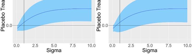
Table 1: Descriptive Statistics

 Ever Treated
 Full Sample
 Subsample
 Standard Standard
 Mean Mean
 Deviation Deviation
 Weather Damage 0.015 0.121 0.156 0.363
 Life Satisfaction 7.937 1.423 7.840 1.506
 Happiness 4.385 1.090 4.301 1.111
 House
 8.008 1.740 7.901 1.807
 Satisfaction
 Job Loss 0.033 0.178 0.039 0.195
 Separation 0.035 0.183 0.038 0.191
 Homeowner 0.691 0.462 0.701 0.456
 Wealth Status 0.700 0.458 0.645 0.478
 Male 0.468 0.499 0.478 0.500
 Age 45.11 18.72 46.42 17.31
 Ever Treated 0.095 0.294 1 0

It’s worth noting that one average respondents have high levels of wellbeing and that
substantially more respondents experienced job loss and separation than experienced
weather‐related house damage.

In the past, the reliability and validity of self‐reported subjective wellbeing among individuals
was assumed10 to validate the use of this measure in groups, with the underlying assumption
being that validity at the individual level ensured validity at the aggregate level. Effectively, it
was believed that the aggregated wellbeing score of Group 1 could be compared to the
aggregated utility score of Group 2. However, more recently, this has become a point of
contention, with the discussion centring around the legitimacy of ranking aggregated ordinal
data.

It is widely accepted that subjective wellbeing data is ordinal, rather than cardinal, in nature.
Despite this, a significant proportion of happiness researchers treat subjective wellbeing data
as cardinal and thus use ordinary least squares to perform their analysis (Schröder & Yitzhaki,
2017). Researchers who are unwilling to assume cardinality instead usually use ordered probit
or logit models in their research. Typically though, ordinal models have returned similar
estimates to cardinal methods (Ferrer‐i‐Carbonell & Frijters, 2004). Overall, the similarity of

10
 This assumption was often implicit rather than explicit.

 7

empirical results between cardinal and ordinal models has led many to conclude that, for
subjective wellbeing data, the distinction between cardinality and ordinality is unimportant
(Schröder & Yitzhaki, 2017).

Recent literature has challenged this assumption, showing that common models may produce
unreliable results when applied to ordinal data. Bond & Lang (2019) show that it is effectively
impossible to rank two groups in order of happiness. A monotonic transformation which is
rank preserving at the individual level can almost always be found which will change the rank
at a group level11. This also means that two monotonic transformations which are individually
rank preserving can be found which provide coefficient estimates of the opposite sign. We
provide a simple two‐person example of this in Table 2. At the original scale, the group means
of Group 1 and Group 2 are identical. However, this is fragile to a change in the underling
scale. Applying a monotonically increasing convex transformation results in Group 1 having a
higher mean than Group 2, while a monotonically increasing concave transformation has the
opposite effect.

Table 2: Data Transformation Example

 Group 1 Group 2
 Convex Concave Convex Concave
 Original Transform Transform Original Transform Transform
 Person A 1 0.1 3.16 5 2.5 7.07
 Person B 9 8.1 9.49 5 2.5 7.07
 Group Average 5 4.1 6.32 5 2.5 7.07

This strong criticism of the reliability of subjective wellbeing data for use in comparing groups
also casts the conclusions of existing studies into doubt. In response to this, several authors
have attempted to defend the robustness of the existing literature and to put forward
alternative methods of analysis for future research using subjective wellbeing data. Chen et
al. (2019) suggest focusing on the median instead of the mean when analysing subjective
wellbeing data, due to the robustness of the median to monotonic rank preserving
transformations. Similarly, they also suggest using the equality of mean and median in
symmetric distributions to reinterpret existing ordered logit and probit models as median,

11
 See Bond & Lang (2014) for an intuitive explanation and further examples. Here, we use σ=0.5 and σ =2.

 8

rather than mean, regressions. This reinterpretation makes the conclusions of many existing
papers robust to the criticism of Bond and Lang (Chen et al., 2019).

An alternative approach is taken by Bloem (2018), who suggests using a series of data
transformations to check the robustness of results obtained using cardinal models. His
research presents two key insights. The first is that passing the theoretical criteria developed
by Schröder & Yitzhaki (2017) and Bond & Lang (2019) is not a guarantee of reliable results.12
While it may be possible there is no monotonic rank preserving transformation that will
reverse the sign of an estimated coefficient, this is no guarantee that valid transformations
will not substantially change both the size and significance of an estimated coefficient. The
second insight is that failing the theoretical criteria does not automatically invalidate the
results obtained, if only relatively extreme transformations substantially influence the results
(Bloem, 2018). Following on from these two insights, Bloem (2018) suggests applying a series
of transformations to the underlying data to check the robustness of results to different
underlying cardinalizations. we apply the transformation suggested by Bloem (2018) which
ensures the endpoints of the data remain numerically unchanged. The transformation is given
by Equation (1):

 (1)
 ∗
 
When σ is exactly equal to one, the transformed scale exactly equals the reported scale. This
means that the “true” distance between reported values of 1 and 2 is assumed to be the same
as the distance between reported values of 9 and 10. For values of σ greater than one, the
scale is assumed to be convex. This means that the gap between reported values of 1 and 2
is assumed to be smaller than the gap between reported values of 9 and 10. For values of σ
less than one, the scale is assumed to be concave, which implies that the gap between
reported values of 1 and 2 is greater than the gap between reported values of 9 and 10. The
transformation process is shown in Figure , where the σ=1 line reflects the original reported
values:

12
 This is ignoring other reasons why research might produce unreliable results such as omitted variable bias and
self‐selection bias. Issues such as these would, of course, result in unreliable results irrespective of the issues
relating to subjective wellbeing data discussed by Bloem (2018), Bond & Lang (2019), and Schröder & Yitzhaki
(2017).

 9

Figure 1: Transformed Variable Example

We apply this transformation to all three dependent variables (life satisfaction, recent
happiness, and satisfaction with the person’s house), using 100 evenly spaced values of σ
between 0.1 and 10. Descriptive statistics for a sample of the transformed variables are
presented in Table 3. We display the within‐person standard deviations as they are the most
relevant.13

Table 3: Transformed Dependent Variables and Within‐Person Standard Deviations (Full
Sample)

 Life Satisfaction
 Life Happiness Satisfaction
 Satisfaction Happiness with House
 Sigma Satisfaction Standard with House
 Standard Mean Standard
 Mean Deviation Mean
 Deviation Deviation
 0.1 9.74 0.11 5.79 0.09 9.73 0.17
 0.5 8.86 0.42 5.08 0.36 8.88 0.58
 1 7.94 0.70 4.39 0.57 8.01 0.93
 5 4.04 1.36 1.93 0.82 4.59 1.78
 10 2.39 1.34 1.05 0.72 3.20 1.88

 IV. Methodology
To examine the impacts of weather‐related disaster events on subjective wellbeing we will
use a Difference‐in‐Difference (DiD) estimation approach. The DiD technique can, under

13
 The within‐person standard deviations show how variable an individual’s subjective wellbeing is over time.

 10

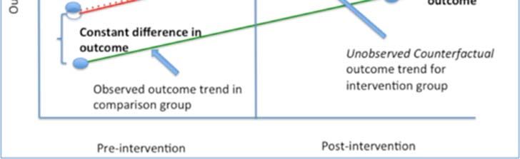
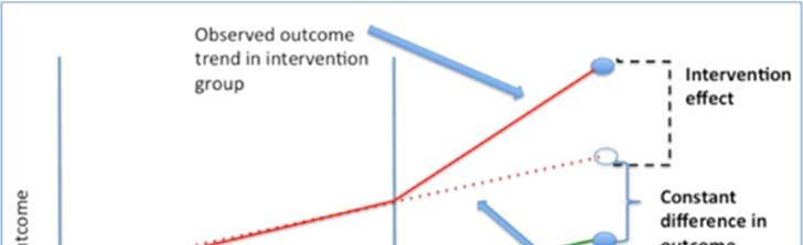
certain assumptions which we will discuss shortly, generate a causal estimate of a treatment
effect.

The simplest version of a DiD analysis consists of two periods of data, with data broken up
into a treatment group and a control group. The two groups can be structurally different
which means they can have different outcomes in the first period. In the first period, neither
group receives a treatment. In the second period, the treatment group receives a treatment
while the control group does not. The outcomes of both groups can change. The treatment
effect is calculated as the change in the treatment group outcome less the change in the
control group outcome14. A visual explanation of the DiD technique is presented in Figure 2.

Figure 2: Difference‐in‐difference Estimation Technique (Columbia Public Health, n.d.).

While the DiD technique is quite flexible, it does require several assumptions on the
underlying data generating process in order for causal estimates to be obtained. In addition
to the assumptions of the ordinary least squares (OLS) technique, four additional assumptions
are required for a DiD approach to be valid: the exogeneity assumption, the no pre‐treatment
effect assumption, the stable unit treatment value assumption (SUTVA), and the common

14
 A key underlying assumption is that, in the absence of no treatment, the treatment group would have
experienced the same change as the control group. This is known as the common trends assumption and is
discussed in some depth in Section Error! Reference source not found..

 11

trends assumption (Lechner, 2010).15 If these four assumptions are met by the underlying
data generating process, the DiD estimator will result in causal estimates.

The exogeneity assumption states that the covariates, or control variables, must be
independent of the treatment status (Lechner, 2010).16 It is easy to see why this must be the
case. Consider the relationships between happiness, weather‐related house damage and
income, where weather‐related house damage is the dependent variable and income is a
covariate. It might seem reasonable to include income as a control variable in the regression,
as it would be expected to influence happiness. Unfortunately, this would violate the
exogeneity assumption. Experiencing weather‐related house damage may be reasonably
expected to change income, resulting in endogeneity and invalid estimates. For this reason,
only control variables which cannot be influenced by the treatment status may be included in
a DiD regression. Clearly, fixed effects based variables pass this criterion, as does the
respondent’s age. However, we do not believe that any other time‐variant variable can be
reasonably assumed to be independent of the treatment status. For this reason, we only
control for age,17 as well as both individual and time fixed effects.

The no pre‐treatment effect assumption states that the treatment must have no effect in the
pre‐treatment period (Lechner, 2010). While this may appear trivially true, it is not actually
the case in some situation. Primarily, this assumption is violated whenever a person can
anticipate treatment or is aware of how they can change their treatment status. We view it
as unlikely that this assumption poses a major issue in this analysis, as it would involve people
being aware when they were going to suffer weather‐related house damage and pre‐
emptively changing their happiness to reflect this.

SUTVA states that an individual’s outcome must only be affected by their individual treatment
status, and not by the treatment status of others around them. SUTVA is satisfied if there are
no spillover or interaction effects between individuals (Lechner, 2010). Two potential

15
 Different authors explain these assumptions in subtly different ways. See Columbia Public Health, n.d. for an
alternative explanation of the DiD assumptions.
16
 As per the standard OLS assumptions, the covariates must also be independent of the outcome variable to
avoid the classic endogeneity issue. The DiD exogeneity assumption is just an extension of this idea. Including
covariates which are endogenous to the treatment status will cause the treatment effect to be “soaked up” by
the covariates, resulting in an invalid estimate of the treatment effect.
17
 We include control variables for both age and age squared to capture any non‐linearities in the relationship
between age and wellbeing.

 12

violations of SUTVA exist in this analysis. Firstly, it is possible that people’s happiness partially
depends on the happiness of people they know. This is intuitively a very reasonable
proposition – it seems likely that your happiness may be influenced by the happiness of your
family, friends, or neighbours. Secondly, utility may be affected by relative quantity rather
than absolute quantity. This would result in a person being affected by the treatment that
other people receive. Suppose your house was not damaged, however the houses across the
road were damaged by a weather‐related disaster.18 The impact of this on your happiness is
unclear. Your happiness may go down, with the intuition being you care about those around
you and thus you become less happy when they experience material loss due to a weather‐
related disaster. Your happiness may remain unchanged, as you have personally suffered no
loss or no gain. Alternatively, your happiness could increase. The charitable explanation of
this would be you feel lucky to emerge unscathed. A considerably less charitable explanation
is that you are now considerably better off relative to those who experienced damage, and
that has increased your happiness. Both happiness interdependence and the influence of
spillover treatment effects would violate SUTVA. The sign and size of these issues are unclear;
however, they seem unlikely to be overly large in comparison to the main effect (of
experiencing weather‐related house damage yourself).

The common trends assumption is widely considered to be the most important DiD
assumption (Angrist & Pischke, 2008; Friedman et al., 2013). For the common trends
assumption to be satisfied, the difference in pre‐treatment outcomes between the treatment
and control group must remain constant over the time period where treatment occurs. This
key assumption is not testable, as the required counterfactual (the outcomes of the treated
group had no treatment occurred) is clearly not observable. However, when a researcher has
several time periods worth of data available, he or she can check whether the treatment and
control groups have common trends in the periods where treatment does not occur using
placebo regressions (Lechner, 2010). While this does not ensure the common trends
assumption is met, it can provide the researcher with a degree of confidence around the likely
validity of the assumption. Of course, the researcher should also consider whether the

18
 Here we are making the unrealistic assumption that the people who were affected by a weather‐related house
damage experienced no loss of happiness in order to highlight the possibility of relative happiness effects. This
means any change in happiness among the control group must solely be due to relative quantities, and not due
to the interdependence of happiness (which is the first potential SUTVA violation we discussed above).

 13

treatment coincides with any other shock which is likely to violate the common trends
assumption. We view that as unlikely to be the case here, as the treatment (experiencing
weather‐related house damage) is “messy” with different people experiencing treatment in
different years.19

The best control group is arguably the group of “ever effected” people who did not experience
treatment in any given particular year. Allowing for some selection into treatment,20 this
control group has the strongest theoretical grounds for being otherwise identical to the
treatment group (the “ever effected” people who did experience treatment in any given
particular year). However, for the same reason21, this control group is also the most likely to
experience the SUTVA violations of happiness interdependence and spillover treatment
effects. For this reason, we conduct a common trends placebo test on both the “ever
affected” control group and the full sample control group, regressing life satisfaction on a
dummy variable which takes the value of one the year before weather‐related house damage
is experienced.22 Results are nearly identical for both samples. At the original scale, where
σ=1, neither placebo regression is significant at the 5% level suggesting subjective well‐being
the year before the house damage is not significantly different from subjective well‐being the
years before that. The full sample placebo becomes significant at the 5% level when σ=0.1 or
σ=3.4, while the “ever affected” sample placebo reaches 5% significance at σ=4. These are
fairly extreme values of σ. Results of the placebo treatment regression are presented in Figure
. Overall, we view it as likely that the common trends assumption holds. In addition, we see
no strong theoretical argument why the common trends assumption should not hold given
the unpredictable nature of extreme weather events.

19
 If all treatment occurred over a very short space of time, it increases the possibility that there could be a
correlation with another sudden event, such as an unrelated policy change, which may cause the outcomes of
the treatment and control groups to diverge irrespective of treatment. This would clearly violate the common
trends assumption.
20
 It seems reasonable to assume that certain locations have a higher weather‐related disaster risk, meaning that
there is some element of selection into treatment status by location selection.
21
 It seems a reasonable assumption that a higher degree of similarity between the treatment and control group
will increase the importance of comparisons between the two groups.
22
 This is just a lead of the weather‐related house damage (WRHD) variable. This regression also includes
dummies for contemporaneous and lags of the weather‐related house damage variable, hence the lead
dummy compares subjective well‐being in the year just before the WRHD to the subjective well‐being in the
years before that.

 14

Figure 3: Placebo Regression for Full Sample and "Ever Affected” Subsample

Summarizing, there are three important considerations when deciding upon an estimation
strategy. Firstly, it remains unclear to what extent different subjective wellbeing variables
measure individual elements of wellbeing as compared to measuring overall wellbeing. A
common example of this is the distinction between happiness and life satisfaction. In the
dataset we use, there is some evidence to suggest they do measure different things with
relatively low correlations between the two variables. The average within‐year correlation of
life satisfaction and happiness is 0.47, while the average within‐person correlation is only
0.20. The second consideration is that the effect of an event on subjective wellbeing may be
heterogeneous, with different groups being affected by treatment differently. This includes
the possibility of heterogeneity arising for selection into treatment,23 which could result in
the “ever treated” group being structurally different24 from the “never treated” group. Finally,
it is problematic to treat subjective wellbeing data as cardinal for the purposes of analysis
(which is commonly done) given almost all authors agree that subjective wellbeing data is
ordinal in nature. As shown by Bond & Lang (2019), this can lead to misleading results which
are fragile to monotone transformations of the underlying subjective wellbeing data.25

23
 It seems reasonable to assume that certain locations have a higher risk of experiencing a weather‐related
event and that people are aware of this.
24
 This difference may be unobservable.
25
 These transformations represent different assumed cardinal scales, as we discussed in some depth in Section
IV.

 15

We employ three techniques in our estimation strategy to mitigate these issues and provide
more robust estimates. Firstly, we use three different dependent variables in our analysis: life
satisfaction (LifeSat), satisfaction with housing (HouseSat),26 and happiness (Happiness).27
The use of both life satisfaction and happiness reduces the risk of a misleading result arising
from measuring a subset of subjective wellbeing rather than overall subjective wellbeing. We
also include satisfaction with housing as it is likely to be the most sensitive to experiencing
weather‐related house damage.28 Secondly, we run the analysis upon both the entire sample
and three different subsets. These subsets are based on treatment status, homeownership
status, and self‐reported prosperity level. This allows for the introduction of heterogeneous
treatment effects. Finally, we employ a series of data transformations as suggested by Bloem
(2018) in order to at least partially mitigate the concerns raised by Bond & Lang (2019).

The model specifications we employ include control variables for age and age squared,29 as
well as both individual and time fixed effects. In addition, all models are run using individual‐
cluster and time‐cluster robust standard errors.30

 V. Results
 a. Weather Related House Damage on Subjective Wellbeing
In this section we present the regression estimates on the effects of weather‐related house
damage (WeatherDamage) on subjective wellbeing (SWB) for both the full sample and the
“ever treated” subsample. Equation (2) presents the main model specification, where the
measure of SWB is alternatively LifeSat(isfaction), HouseSat(isfaction), or Happiness.
Individual and time fixed effects are denoted by and respectively.

 ℎ 1 ℎ 2 (2)
 ℎ 3+ 

26
 This is clearly a subset of overall subjective wellbeing and is not attempting to measure overall subjective
wellbeing.
27
 As mentioned earlier, this question asked the respondent how much time they had been happy within the last
4 weeks.
28
 Satisfaction with housing is quite clearly a subset of overall subjective wellbeing.
29
 We do not include additional control variables. See Section IV for more details.
30
 The standard errors are both individual‐cluster robust and time‐cluster robust. We obtain these using the R
function vcocDC from the package plm. See https://www.rdocumentation.org/packages/plm for more details.

 16

We estimate three different treatment effects. Any impact on subjective wellbeing that
occurs within 12 months of treatment (Year 1) is captured by the term . Similarly, is the
estimate of any impact between 12‐ and 24‐months following treatment (Year 2). Finally, we
allow for a “long run” treatment effect that occurs in all later time periods (Year 3+). Table 4
presents the results obtained from running the model specification in Equation (2).

Table 4: Weather‐Related House Damage on Different Measures of Subjective Wellbeing

 LifeSat HouseSat Happiness
 Year
 Full Ever Full Ever Full Ever
 1 ‐0.03 ‐0.04 ‐0.06 ‐0.08* ‐0.03** ‐0.02
 2 ‐0.08*** ‐0.09*** ‐0.03 ‐0.05 ‐0.01 ‐0.01
 3+ ‐0.02 ‐0.06 0.07* 0.03 ‐0.02 ‐0.01
 Note: * p < 0.1; ** p < 0.05, *** p < 0.01
Experiencing weather‐related house damage is associated with a small but statistically
significant decrease in life satisfaction in the 12‐24‐month period (Year 2) after the weather
event occurs. For the full sample, we estimate life satisfaction decreases by 0.08 points. For
the “ever affected” sample, we estimate life satisfaction decreased by 0.09 points. Both
estimates are statistically significant at the 1% level. Otherwise, we estimate results which are
generally insignificant with no other estimated coefficient significant at the 1% level. When
using house satisfaction as the dependent variable, not a single estimated coefficient is
significant at the 5% level, and only two estimate coefficients are significant at the 10% level.
When using happiness as the dependent variable, only a single coefficient is significant at
either the 5% or the 10% level. Finally, there is no clear systemic difference between estimates
obtained when using the full sample and those obtained when using the “ever treated”
subsample.

While the results are generally insignificant, it should be noted that the estimates are almost
always negative. Still, magnitudes of all 18 estimated coefficients are small relative to the
mean and variance31 of the respective variables. These are presented in Table 5 below. Table

31
 Here we refer to the within‐person variance. When considering how small or large the estimated treatment
effect is, what matters is not the variance of wellbeing across people, but how variable an individual’s wellbeing
is over time.

 17

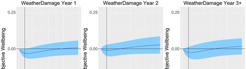
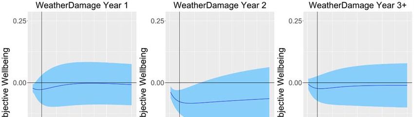
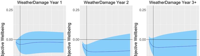
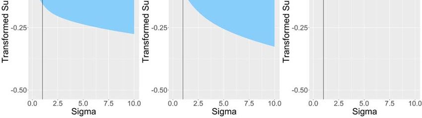
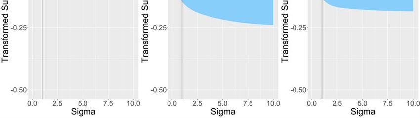
6 presents the coefficient estimates as a percentage of the average within‐person standard
deviation.

Table 5: Mean and Standard Deviation of Subjective Wellbeing Measures

 Full Sample Ever Treated Sample
 Standard Standard
 Mean Mean
 Deviation Deviation
 LifeSat 7.94 0.70 7.84 0.84
 HouseSat 8.01 0.93 7.91 1.13
 Happiness 4.39 0.57 4.30 0.66

Table 6: Effect of Experiencing a Weather‐Related Natural Disaster as a Percentage of
Within‐Person Standard Deviation of Subjective Wellbeing

 LifeSat HouseSat Happiness
 Year
 Full Ever Full Ever Full Ever
 1 3.96% 4.93% 6.91% 7.12%* 5.37%** 3.75%
 2 11.06%*** 11.20%*** 3.55% 4.28% 1.90% 0.98%
 3+ 3.35% 6.98% 7.14%* 2.91% 4.28% 2.01%
 Note: * p < 0.1; ** p < 0.05, *** p < 0.01

The largest impacts on both life satisfaction occur in the year following experiencing weather‐
related house damage, while happiness is generally more affected in the year of treatment.
The overall estimated effect is fairly small, with no treatment coefficient explaining over
11.2% of the within‐person standard deviation on subjective wellbeing.

We now carry out a robustness check of our main model estimates by applying the data
transformation suggested by Bloem (2018). It is important to note that any such
transformation will affect both the mean and the distribution of the data and thus the
resulting coefficient estimates and p‐values. Section III provides an overview of how the mean
and within‐person standard deviation change when the transformation is applied. We
present the regression results of the transformed data below. The full sample and “ever
affected” sample estimates of weather‐related house damage on life satisfaction are
displayed in Figure 4 and Figure 5. The full sample and “ever affected” sample estimates of
weather‐related house damage on satisfaction with housing are displayed in Figure 6 and
Figure 7. Finally, the full sample and “ever affected” sample estimates of weather‐related
house damage on happiness are displayed in Figure 8 and Figure 9. All figures display both
the point estimate and the 95% double‐cluster robust confidence interval.
 18

In general, the estimates are all robust to transformations of the assumed underling cardinal
scale and the assumption of a different scale would not change the conclusions drawn above.
Interestingly, the Year 2 estimate of weather damage on life satisfaction is moderately fragile
to the transformation. The full sample estimate becomes insignificant at the 1% level at σ=1.8
and insignificant at the 5% level at σ=3.1. The “ever affected” sample estimate becomes
insignificant at the 1% level at σ=2.7 and insignificant at the 5% level at σ=3.9. These are not
unreasonable transformations. A σ value of 1.8 implies that that a person who reports a
wellbeing score of 10 has about 3.5 times the wellbeing as someone who reports a score of
5, rather than double the wellbeing as the untransformed cardinal scale would imply. A σ
value of 2.7 implies this difference is about 6.5 times. Other estimates either remain
statistically insignificant or rapidly lose significance. For example, the Year 1 full sample
estimate of weather damage on happiness loses 5% significance at σ=1.1 and loses 1%
significance at σ=1.9.

Overall, while the effect of weather damage on life satisfaction is statistically significant, it is
fairly small in magnitude. The estimates of weather damage on satisfaction with housing and
happiness are generally both statistically insignificant and small in magnitude. Applying the
data transformation generally makes results less statistically significant, with the estimates of
weather damage on life satisfaction losing 1% significance at fairly moderate transformations.

Figure 4: Weather‐Related House Damage on Transformed Life Satisfaction (Full Sample)

 19

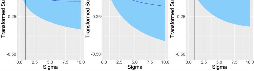
Figure 5: Weather‐Related House Damage on Transformed Life Satisfaction (Ever Affected
Sample)

Figure 6: Weather‐Related House Damage on Transformed Satisfaction with Housing (Full
Sample)

 20

Figure 7: Weather‐Related House Damage on Transformed Satisfaction with Housing (Ever
Affected Sample)

Figure 8: Weather‐Related House Damage on Transformed Happiness (Full Sample)

 21

Figure 9: Weather‐Related House Damage on Transformed Happiness (Ever Affected Sample)

 b. Major Life Events on Subjective Wellbeing
We showed so far that experiencing weather‐related house damage results in relatively small
and mostly insignificant effects on subjective wellbeing, whether measured by life satisfaction
or happiness. The question naturally arises as to whether any life event affects subjective
wellbeing, or whether the majority of variance in subjective wellbeing is essentially random
in nature. In this section we compare the effect from experiencing weather‐related house
damage (WeatherDamage) on subjective wellbeing to the effects from experiencing either
long‐term relationship breakup (Separation) or involuntary loss of job (JobLoss)32 on
subjective wellbeing. As in Section a, results are presented for both the full sample and the
“ever treated” subsample (all those who have ever experienced weather‐related house
damage), and we use both group and time cluster‐robust standard errors. Equation (3)
presents the main model specification, where EVENT is alternatively Separation, JobLoss, or
WeatherDamage.33

32
 An involuntary loss of job includes both being fired and being made redundant.
33
 The random element in weather related house damage is likely to be bigger than the random element in job
loss and separation. Hence, the estimates of the impact of weather related damage are more likely to be
unbiased than the estimates of the impact of job loss and of separation. A priori, it’s hard to say, however, in
what direction the bias would be.

 22

 1 2 3+
 (3)
 
The interpretation of all coefficients is the same as for Equation (2) in Section a on page 16.
The results from estimating Equation (3) are presented below. Here, the full sample is almost
certainly the better comparison group, as any heterogeneity arising from selection into
treatment34 seems unlikely to affect how the individual would respond to a different life
event. Additionally, the use of the “ever treated” sample results in a significant reduction of
the number of observations. In the full sample of 144,784 observations, there are 5,033
instances of a long‐term relationship breakup and 4,320 instances of an involuntary loss of
job. In the “ever affected” sample of 13,809 observations, there are only 524 instances of a
long‐term relationship breakup and 544 instances of an involuntary loss of job. The “ever
affected” sample results are thus presented mainly for consistency. However, on the whole
they are fairly similar to the full sample estimates.

 i. Major Life Events on Life Satisfaction
In this section we present the estimates of major life events on life satisfaction. Table 7
presents the coefficient estimates, while Table 8 presents the estimates as a percentage of
within‐person standard deviation.

Table 7: Major Life Events on Life Satisfaction

 WeatherDamage Separation JobLoss
 Year
 Full Ever Full Ever Full Ever
 1 ‐0.03 ‐0.04 ‐0.34*** ‐0.39*** ‐0.15*** ‐0.24***
 2 ‐0.08*** ‐0.09*** ‐0.08*** ‐0.03 ‐0.05*** ‐0.08
 3+ ‐0.02 ‐0.06 0.04* ‐0.01 0.01 ‐0.12
 Note: * p < 0.1; ** p < 0.05, *** p < 0.01

34
 A treated unit is one who experiences weather‐related house damage.

 23

Table 8: Major Life Events as a Percentage of Within‐Person Standard Deviation of Life
Satisfaction

 WeatherDamage Separation JobLoss
Year
 Full Ever Full Ever Full Ever
1 3.96% 4.93% 48.24%*** 47.02%*** 21.57%*** 28.28%***
2 11.06%*** 11.20%*** 11.75%*** 3.89% 7.10%*** 9.30%
3+ 3.35% 6.98% 5.87%* 1.64% 1.47% 14.58%
Note: * p < 0.1; ** p < 0.05, *** p < 0.01

For the full sample, the Year 1 effect from experiencing a long‐term relationship breakup is
an 0.34‐point reduction in life satisfaction, which corresponds to 48% of a within‐person
standard deviation. The Year 2 effect is an 0.08‐point reduction, or 11% of a within‐person
standard deviation. Year 3+ effects are insignificant at the 5% level. For the “ever treated”
sample, the estimates are similar. The Year 1 effect is an 0.39‐point reduction in life
satisfaction, which corresponds to 47% of a within‐person standard deviation. Year 2 and Year
3+ effects are statistically insignificant.

The effect of involuntary loss of job is less severe, but still significant and large in magnitude.
For the full sample, the Year 1 effect is an 0.15‐point reduction in life satisfaction, while the
Year 2 effect is an 0.05‐point reduction. These estimates correspond to 21% and 7% of a
within‐person standard deviation. Year 3+ effects are again insignificant. For the “ever
treated” sample results are also generally similar. The Year 1 effect is an 0.24‐point reduction
in life satisfaction, which is 28% of a within‐person standard deviation. Year 2 and Year 3+
effects are statistically insignificant.

Overall, experiencing weather‐related house damage only has a small effect on life
satisfaction. Weather‐related house damage is never estimated to explain more than 11.2%
of a within‐person standard deviation. In contrast, both separation and job loss have much
larger effects on life satisfaction. In particular, The Year 1 effect of experiencing separation is
estimated to be over 45% of a within‐person standard deviation for both the full sample and
“ever treated” group. The Year 1 effect of experiencing job loss is estimated to be over 21%

 24

of a within‐person standard deviation for both the full sample and “ever treated”
subsample.35

 ii. Major Life Events on Happiness
In this section we present the estimates of major life events on happiness. Table 9 presents
the coefficient estimates, while Table 10 presents the estimates as a percentage of within‐
person standard deviation.

Table 9: Major Life Events on Happiness

 WeatherDamage Separation JobLoss
 Year
 Full Ever Full Ever Full Ever
 1 ‐0.03** ‐0.02 ‐0.16*** ‐0.05 ‐0.07*** ‐0.08**
 2 ‐0.01 ‐0.01 0.00 ‐0.02 ‐0.03 ‐0.09
 3+ ‐0.02 ‐0.01 0.07 0.10* ‐0.02* ‐0.11***
 Note: * p < 0.1; ** p < 0.05, *** p < 0.01

Table 10: Major Life Events as a Percentage of Within‐Person Standard Deviation of
Happiness

 WeatherDamage Separation JobLoss
 Year
 Full Ever Full Ever Full Ever
 1 5.37%** 3.75% 28.01%*** 7.67% 12.47%*** 11.82%**
 2 1.90% 0.98% 0.87% 3.40% 5.77% 13.25%
 3+ 4.28% 2.01% 12.76% 15.19%* 3.40%* 15.84%***
 Note: * p < 0.1; ** p < 0.05, *** p < 0.01

For the full sample, the Year 1 effect from experiencing a long‐term relationship breakup is
an 0.16‐point reduction in happiness, which corresponds to 28% of a within‐person standard
deviation. The Year 2 and Year3+ effects are statistically insignificant. For the “ever treated”
sample, all three coefficient estimates are insignificant at the 5% level. Interestingly, both the
full sample and “ever affected” sample have positive Year3+ coefficient estimates which are
similar to full sample Year 3+ estimate of separation on life satisfaction. It certainly seems
possible that, after a short period of unhappiness arising from the end of a long‐term

35
 These results are generally robust to applying the transformations discussed in Section 3. Detailed results
are available upon request.

 25

relationship, an individual gains in happiness from having left a relationship where
presumably at least one partner was unhappy.36

For the full sample, the Year 1 effect from experiencing involuntary loss of job is an 0.07‐point
reduction (significant at the 1% level), which corresponds to 12.47% of a within‐person
standard deviation. Year 2 and Year3+ effects are insignificant at the 5% level. For the “ever
affected” sample, the Year 1 effect is an 0.08‐point reduction (significant at the 5% level),
which corresponds to 11.82% of a within‐person standard deviation. The Year 2 effect is
insignificant. Interestingly, the Year 3+ effect is an 0.11‐point reduction (significant at the 1%
level). Irrespective of whether looking at the full sample or the “ever treated” subsample, the
estimated effects on happiness from experiencing either a relationship breakup or
involuntary loss of job are almost always larger than those of experiencing weather‐related
house damage.

Overall, the effect on happiness is similar, although often slightly smaller in magnitude, to the
effect on life satisfaction. Weather‐related house damage has small (no more than 6% of a
within‐person standard deviation) and insignificant effects, while both separation and
involuntary job loss have larger and more significant effects. As found earlier, a long‐term
relationship breakup has the largest impact on happiness (28% of a within‐person standard
deviation for the full sample). Also, as earlier, the “ever treated” sample seems to be more
negatively impacted by involuntary job loss than the full sample, especially in the long
term.37,38

 iii. Major Life Events on Satisfaction with Housing
In this section we present the estimates of major life events on satisfaction with housing.
Table 11 presents the coefficient estimates, while Table 12 presents the estimates as a
percentage of within‐person standard deviation.

36
 There is unfortunately no way to ascertain whether the individual was the person choosing to end the
relationship or not.
37
 Significance levels are once again mixed.
38
 The conclusions drawn are mostly robust to the transformation described in section 3, though it should be
noted that the full sample Year 1 estimate of involuntary job loss is moderately fragile to this transformation.
At σ=5.2, it becomes insignificant at the 1% level, and by σ=7.5 it becomes insignificant even at the 10% level.
However, these are fairly extreme transformations.

 26

Table 11: Major Life Events on Satisfaction with Housing

 WeatherDamage Separation JobLoss
 Year
 Full Ever Full Ever Full Ever
 1 ‐0.06 ‐0.08* ‐0.20*** ‐0.25*** 0.00 0.00
 2 ‐0.03 ‐0.05 ‐0.07* ‐0.05 ‐0.02 ‐0.06
 3+ 0.07* 0.03 0.04 0.08 0.00 ‐0.16**
 Note: * p < 0.1; ** p < 0.05, *** p < 0.01

Table 12: Major Life Events as a Percentage of Within‐Person Standard Deviation of
Satisfaction with Housing

 WeatherDamage Separation JobLoss
 Year
 Full Ever Full Ever Full Ever
 1 6.91% 7.12%* 21.97%*** 21.80%*** 0.43% 0.18%
 2 3.55% 4.28% 7.71%* 4.81% 1.93% 5.09%
 3+ 7.14%* 2.91% 4.44% 7.10% 0.38% 14.53%**
 Note: * p < 0.1; ** p < 0.05, *** p < 0.01

As previously discussed, the impact of experiencing weather‐related house damage on
satisfaction with housing is generally small in both magnitude and significance. For both the
full and “ever treated” sample, no estimate is larger than 8% of a within‐person standard
deviation, and no estimate is significant at even the 5% level. However, the effects of a long‐
term relationship breakup are both larger in magnitude and statistical significance. For the
full sample, the Year 1 estimate is an 0.20‐point reduction in house satisfaction (21 % of a
within‐person standard deviation). It is significant at the 1% level. For the “ever treated”
sample, the Year 1 estimate is an 0.25‐point reduction in house satisfaction (21% of a within‐
person standard deviation), which is significant at the 1% level. For both the full sample and
the “ever treated” sample, neither the Year2 nor Year 3+ estimates are significant at even the
5% level.

For the full sample, involuntary job loss results in small and insignificant estimates. For the
“ever treated” sample, the Year 1 and 2 effects are both insignificant. Interestingly the Year
3+ estimate is fairly large (‐0.16 or 14% of a within‐person standard deviation) and is
significant at the 5% level. This is similar to the previously discussed results where the “ever
treated” sample seems to be more negatively affected by loss of job, especially in the long
term.

 27