Scholarship@Western Western University
←
→
Page content transcription
If your browser does not render page correctly, please read the page content below
Western University
Scholarship@Western

Centre for Human Capital and Productivity.                         Economics Working Papers Archive
CHCP Working Papers

2020

2020-1 The Millennials' Transition from School-to-Work
Audra J. Bowlus

Yuet-Yee Linda wong

Follow this and additional works at: https://ir.lib.uwo.ca/economicscibc

   Part of the Economics Commons

Citation of this paper:
Bowlus, Audra J., Yuet-Yee Linda wong. "2020-1 The Millennials' Transition from School-to-Work." Centre
for Human Capital and Productivity. CHCP Working Papers, 2020-1. London, ON: Department of
Economics, University of Western Ontario (2020).
The Millennials’ Transition from School-to-Work

                              by

           Audra Bowlus and Yuet-Yee Linda Wong

      Working Paper #2020-1                  March 2020

Centre for Human Capital and Productivity (CHCP)
               Working Paper Series

                  Department of Economics
                    Social Science Centre
                     Western University
                  London, Ontario, N6A 5C2
                           Canada
The Millennials’ Transition from School-to-Work∗
† ‡
Audra Bowlus Yuet-Yee Linda Wong
University of Western Ontario Binghamton University
March 30, 2020
Abstract
We present the first study of the high school-to-work transition for American Mil-
lennial males and females. Using data from the PSID Transition to Adulthood from
2005-2011, we estimate the Burdett and Mortensen (1998) model and study changes
between Generation X and Millennials. We find convergence in racial differences in
transition patterns across the generations and in gender earnings by the Great Reces-
sion. These patterns are driven by a large decline in search efficiencies for white males.
Finally, we show the labor market deteriorated for high school graduates prior to, with
a further decline during, the Great Recession.
Keywords: Millennials, school-to-work, search frictions, early career outcomes
∗
This paper was written in memory of George R. Neumann, who supervised both our dissertations and
continued as a mentor and friend until his death. May he rest in peace. We thank Phuong Vu for her helpful
research assistance.
†
Corresponding author. Email: abowlus@uwo.edu
‡
Email: yywong01@gmail.com1 Introduction
The Millennials are often described as the unluckiest generation. Born
between the early 1980s and the late 1990s, this generation is named for
having come of age in the early 2000s, a decade of turmoil that started
with the 9/11 attacks and ended with the Great Recession. Compared to
previous generations the Millennials are the most educated, but also face
the highest unemployment rates, highest educational debt load, lowest
wage growth, and highest rates of living at home with their parents. For
many, they are seen to have had difficulty in making the transition to
adulthood including secure employment, marriage, and home ownership.
Their poor early career labor market performance is often cited by the
press as a reason.1
Among the components to labor market success, the school-to-work
transition is unmistakably important.2 The first school-to-work papers
used the 1979 National Longitudinal Survey of Youth (NLSY-79) and
search models to study the unemployment duration following high school
graduation and subsequent wages and durations of first jobs.3 These pa-
pers studied only males with a particular focus on explaining differences in
the transition between black and white males. More recently, the school-
to-work transition literature has explored the effects of graduating during
different states of the business cycle and has found long-term negative
effects of graduating during a recession.4
1
For evidence and discussion of the Millennials, see Berridge
(2014), Lusardi and Scheresberg (2015), BLS (2014) https://www.
bls.gov/opub/mlr/2014/beyond-bls/millennials-after-the-great-recession.
htm, and WSJ (2015) https://blogs.wsj.com/briefly/2015/11/25/
5-facts-to-silence-your-smug-millennial-nephew-this-thanksgiving.
2
Early labor market mobility, in particular, is thought to affect subsequence wage
growth over one’s life cycle. See, for example, Topel and Ward (1992).
3
These included Wolpin (1987, 1992), Eckstein and Wolpin (1990, 1995) and Bowlus,
Kiefer and Neumann (2001).
4
Examples include Kahn (2010), Genda, Kondo and Ohta (2010), Oreopoulos, von
Wachter and Heisz (2012), and Schwandt and von Wachter (2019).
1In this paper, we revisit the school-to-work transition with a focus on
Millennials. While much has been made of the labor market outcomes of
the college-educated Millennials, little is known about those who graduate
from high school but did not go on to college. Thus, we focus on the
transition for Millennial high school graduates. Our school-to-work model
is based on the canonical equilibrium job search framework of Burdett
and Mortensen (1998), hereafter BM, and our estimation method is from
Bowlus, Kiefer and Neumann (2001), hereafter BKN. We estimate the
model for male and female Millennials providing the first gender-based
comparisons of the school-to-work transition for the U.S. in addition to
race-based comparisons. Going further, we explore how the school-to-
work transition has changed over time. First, we assess the transitions
and earnings outcomes of Millennials with reference to Generation X. In
particular, we compare the experiences black and white male high school
graduates across the two generations. Finally, in line with the more recent
literature on business cycle effects, we examine within the Millennials the
differences in the school-to-work transitions between those who graduated
before the Great Recession and those who graduated during the Great
Recession.
To conduct our analysis, we use education and employment history
data from the Panel Study of Income Dynamics Transition to Adulthood
(PSID-TA) file. We focus on youths who were between 14 and 21 in 2005
and follow them through 2011. As was true for the NLSY-79, the PSID-TA
is uniquely suited to study the school-to-work transition, because it allows
for the construction of completed education and employment histories.
One distinguishing feature of the PSID-TA is that is contains infor-
mation on job search starting time. In particular, it documents whether
and when job search started while respondents were still in school. This
information is often missing in data sets used to study the school-to-work
transition, which is problematic because a non-trivial fraction of students
are often found to have started working before their graduation or imme-
2diately upon graduation. Without record of their search period prior to
accepting the job or prior to graduation even if they have not found a job
by graduation, researchers face a classic initial condition problem.
With this information, we are able to explore its implications. In par-
ticular, we can test whether knowledge of this information changes the
estimates regarding the arrival rates of job offers while unemployed as
well as investigate the various solutions offered to solve the initial condi-
tion problem. Interestingly, we find evidence in support of the solution
proposed by BKN to only use the unemployment spells following gradu-
ation for those who do not take up employment prior to or immediately
after graduation rather than ‘adjusting’ the unemployment durations to
handle the 0 duration spells and the time spent searching while in school.5
In essence BKN used only the forward recurrence times. Under the as-
sumption that the durations are distributed exponentially, the forward
recurrence times (as well as the backward recurrence times) are also dis-
tributed exponentially with the same parameter.6 Thus, BKN argued that
the forward recurrence times would recover the underlying true parameter.
Our test results concur. For black and white males and black females the
exponential distribution is accepted and the exponential parameters re-
covered using the full duration data and the forward recurrence time only
data are not statistically different. The only exception is white females
for which the exponential distribution is rejected. Even so, the parameter
5
The BKN approach is similar to Wolpin(1992) who started the labor market his-
tories in the period after graduation implicitly ignoring the employment spells while in
school and at the time of graduation. Eckstein and Wolpin (1990, 1995), Wolpin (1987)
and van der Klaauw and van Vuuren (2010) are examples of papers that have assumed
a period of search for all 0 length unemployment spells or that have augmented all
unemployment spells with a fixed period of search during school. Our data indicate
that there is a lot of heterogeneity in search periods during school such that assuming
the same period for all would be quite inaccurate.
6
This is due to the memoryless nature of the exponential distribution and is unique
to that distribution. Duration models that contain duration dependence require knowl-
edge of the full duration in order to estimate the underlying parameters of the distri-
bution.
3estimates for the full durations and the forward recurrence times are not
statistically different for white females.
Based on the sample we construct, we document the school-to-work
patterns for male and female high school graduates, separately for whites
and blacks.7 While the differences are not large, we find that females have
shorter unemployment durations, longer job spells and a slightly higher
chance of making a job-to-job transition following their first job spell.
Despite more favorable transition patterns for females, mean monthly ac-
cepted earnings on the first job is higher for males. There are also very
few differences for each sex group between blacks and whites indicating
that for high school graduates racial differences have for the most part
converged for the Millennials, at least in terms of the school-to-work tran-
sition.
Driven by the evidence that it takes time to find jobs after graduation
and that the gender earnings gap persists despite favorable search pro-
cesses for females relative to males, we adopt and estimate BM’s general
equilibrium search model. The model allows us to better understand and
quantify the search frictions faced by graduates as they transition to work
as well as how those frictions affect wages and wage dispersion through
firms’ wage posting decisions. It also gives a measure of the amount of
monopsony power held by firms and how it may vary across groups or over
time.
Our estimates show that females have higher job arrival rates while
unemployed and a lower exogenous job destruction rate than males. White
females also see higher job arrival rates while on the job than white males,
while black females do not find jobs as quickly as black males while on
the job. Normalizing the job offer arrival rates by the exogenous job
destruction rate, however, both white and blacks females are more efficient
than white and black males, respectively, in entering and moving up the
wage ladder. Yet, mean earnings for females is less than males.
7
In this way we follow BKN which is useful for comparison purposes.
4We explore the male-female earnings gap by asking what would the
outcomes have been for females if they had faced their search parameters
but the firm productivity distribution of the males. Re-solving the equilib-
rium model, we find that the male-female earnings gap on first jobs would
close in this case. This indicates that the gender earnings gap is due to
productivity differences across males and females. This result is similar
to Bowlus (1997), who found that 70-80% of the male-female earnings
gap was due to productivity differences among new entrants to the labor
market in the early 1980s.8 One difference is that Bowlus (1997) focussed
only on full-time jobs, while in this study we include part-time jobs with
more than 20 hours/week. Given the females in our sample are much more
likely to hold part-time jobs than the males, this may in part explain why
productivity differences explain the male-female earnings gap.
Next, to determine how the labor market has changed over time, we
compare the male Millennial results to the patterns found in BKN, who
studied black and white male high school graduates using data from the
NLSY-79. That data set covered those who were born in the early to
mid 1960s and came of age in the late 1970s and early 1980s, the start
of Generation X. We find that, compared to males from Generation X,
Millennial males are far less likely to hold a job at graduation, take longer
to find their first jobs, have shorter job durations, and are less likely to
make a job-to-job transition following their first job and rather end up
returning to unemployment. These differences indicate male Millennials
faced greater search frictions and, hence, firms had more monopsony power
during this period and were able to compress earnings as a result.
8
Bowlus(1997) does not study the school-to-work transition but rather the transi-
tions following the first full-time job with a focus on females leaving the labor market
for child care reasons. In our data we find females are no longer exiting the labor force
following the first job and, therefore, we do not focus on this issue. Rather we are
interested in gender differences in the initial transition from school-to-work and are the
first to focus on this transition for females.
5Comparing the BM model estimates shows that the search frictions
faced by male Millennials during their school-to-work transition were sub-
stantially higher than those found by BKN for Generation X males. In
particular, both black and white male Millennials faced substantially lower
arrival rates while unemployed. White males also saw their arrival rate
of offers while employed fall significantly and their job destruction rate
increase. In fact, unlike the case of Generation X where BKN found the
white males outperformed the black males in every search dimension, we
find that for the Millennials the labor market for white males has de-
teriorated so much more so than it has for black males that the white
and black male high school graduates faced much more similar search pa-
rameters in the early mid 2000s. There are even some dimensions, e.g.
on-the-job search, in which the black males now out perform the white
males. Thus, over time racial differences in the school-to-work transition
have converged. However, the convergence was not one that brought up
the black male high school graduates to their white counterparts. Instead,
both groups saw their labor markets deteriorate with the white male high
school graduates converging down to their black counterparts.
Given the estimated firm productivity levels for the 2000s, we examine
what the Millennial males’ school-to-work transition would have looked
like, i.e. how much better would it have been, if they had faced Generation
X’s lower search frictions. While both white and black males show higher
earnings levels, this is particularly true for the white males. The higher
earnings levels come from three sources: (1) increased reservation wages
of the workers due to higher arrival rates of offers while unemployed, (2)
decreased monopsony power of the firms as more competition due to higher
arrival rates while employed and lower job destruction rates forces them to
offer higher wages in the new equilibrium; and (3) higher earnings growth
through on-the-job search because worker move up the job ladder faster
due to higher offer rates while employed.
6Finally, we study how the labor market for the Millennials changed
within the generation by exploring the impact of the Great Recession
on males and females.9 We find that males and females who graduated
during the Great Recession had substantially longer unemployment dura-
tions, shorter job durations, lower earnings and lower job-to-job transition
rates than those who graduated before the Great Recession. The search
estimates reveal that the relative position of females improved during the
Great Recession even though it declined for both males and females. This
is true even for the male-female earnings gap for first jobs after gradua-
tion, which completely closes. Thus, overall, we find a story of racial and
gender convergence for Millennial high school graduates. Unfortunately
it is convergence to a much lower earnings and search effectiveness level.
As more data become available it will be interesting to see whether the
school-to-work transition improved for future generations as the economy
recovered from the Great Recession as well as whether the gaps reemerged.
The paper is organized as follows. Section 2 discusses the data and
presents sample statistics for Millennial males and females. Section 3
briefly presents the BM model and the BKN estimation method. Section
4 presents the estimation results for Millennial males and females, while
Section 5 explores the differences across Generation X and Millennials for
males. The impact of the Great Recession on the school-to-work transi-
tions of the Millennials is examined in Section 6. Section 7 concludes.
2 Data
As mentioned above, we use data from the PSID-TA to study the early
labor market outcomes of the Millennials. In the PSID-TA, respondents
are surveyed biannually to present. We use the years from 2005 to 2011.
9
Here we combine blacks and whites and divide the sample only by sex. This allows
us to have large enough sample sizes of those who graduated before the Great Recession
and those who graduated during the Great Recession.
7The PSID-TA file contains respondents’ employment status, job history
up to five jobs, non-employment status retrospectively on a monthly basis,
income, and demographic information such as marital status, education
attainment, and occupation. However, the file does not contain basic
information such as age, sex, and race. To obtain this information, we
link the sample to the ‘individual files’ of the PSID. Time is denominated
in months in the PSID-TA files.
We restrict our sample to a fairly homogeneous group. We extract
youths who were between 14 and 21 years old in 2005, and follow them
through the 2011 interview. Further, we restrict our analysis to male
and female high school graduates who are either black or white. In what
follows, we describe how the sample was constructed and then provide
sample characteristics.
2.1 Sample Construction
As a first step, we must determine the highest level of schooling attained
in order to select those who have only attained a high school degree. Un-
fortunately, the 2005 and 2007 surveys do not contain information on the
highest grade attained. Therefore, to assign the highest level of schooling
completed for each respondent as well as the date of completion, we make
use of the information recorded on the month and year of completing high
school and the monthly enrollment status variable.
We exclude respondents who graduated before 2004, because there is
no employment history recorded prior to 2004. We also exclude respon-
dents whose education was ongoing through the 2011 interview or was
followed by non-response in subsequent interviews such that an end date
as well as a highest level could not be determined. Finally, we drop respon-
dents who had missing or inconsistent information such that the highest
schooling level and/or graduation month and year could not be assigned.
8Next, we construct each respondent’s employment history. The PSID-
TA file collects respondent’s unemployment and out of the labor force
status each month retrospectively for 24 months in the 2007, 2009 and
2011 surveys and for 12 months in the 2005 survey. In addition, it collects
job history information by asking respondents the start and stop months
and years of the five most recent jobs held. While the five recorded jobs
are in no particular chronological order, and can be missing from one inter-
view to another, start and stop months and years were recorded for each
job. Together with the 24-month retrospective non-employment record,
the job spell data provide enough information to construct an initial un-
employment spell following graduation, the length of the first job spell and
its monthly earnings and the first transition following the first job spell.
2.2 Unemployment Durations
We follow BKN and others and do not distinguish between unemployment
and out of the labor force.10 We treat the unemployment duration as the
elapsed time between the start of job search and the end of it when a
‘real’ job is found.11 Here we define a ‘real’ job to be a job with at least 20
hours/week and a duration of at least 3 months.12 If the ‘real’ job starts
10
Separating unemployment from out of the labor force may add noise to the du-
ration data as some respondents reported multiple unemployment spells and multiple
transitions between unemployment and out of the labor force. In addition, as noted
above, we find little need for a non-participation state for females unlike in Bowlus
(1997).
11
The term ‘real’ job was first used in this context by Wolpin (1987).
12
Many labor studies, including BKN, use 35 or 30 hours/week as the minimum
hours needed to be a ‘real’ job. However, in this sample, many respondents did not
report hours worked or were not consistent in their reports. As a means to retain a
reasonable number of school-to-work transitions, we lowered the limit to at least 20
hours per week. In particular, had we used 35+hours/week as our criterion, the sample
would have contained respondents with higher unemployment durations (from about
12 to 20 months, on average, for both males and females). In addition, since many
respondents never report having a 35+hour/week job, the majority of respondents who
worked [20,35) hours would be right-censored (raising the overall censoring rate to over
0.50 for both sexes).
9prior to graduation, we follow BKN and others and require it to last at
least two months after graduation to rule out summer and temporary jobs.
We also require that it be held less than 12 months prior to graduation.
Further, we follow BKN and require respondents to find a ‘real’ job within
three years of graduation.13
It is possible to only partially observe unemployment duration. This
is the case if the start of job search is unknown (left-censoring) and/or the
end of it is unknown (right-censoring). When the start of job search is
unknown, there is a classic initial conditions problem. As we mentioned in
the Introduction, the PSID-TA collected information on job search during
school and so this problem is mitigated in our setting. We are able to use
this information to construct the full unemployment duration prior to the
first job. If the respondent has a ‘real’ job at graduation but does not
report any search activity prior to the start of the job, then we exclude
them from the sample.14
Since time spent searching in school is rarely recorded in surveys, we
present in Figure 1 a histogram for the search durations prior to graduation
or the backward recurrence times. Around 39 per cent of the male sample
reported that they searched while in school. For females 20 per cent
searched before graduation. Of males and females who did search prior to
graduation, 80 per cent searched between one to five months.
13
There are 8 males and 28 females who were unemployed longer than 36 months and
removed from the sample. The higher number for females is due to a greater tendency
for females to be out of the labor force following graduation, although the rate is much
lower for the female Millennials than for past generations. We performed a sensitivity
check and compared results for including these observations and excluding them and
found the findings regarding the distributions of unemployment spells to be robust.
We note that if we had increased the minimum hours requirement to 35, the number of
respondents who searched for a job for three years or more would have increased to 67
cases for males and 101 cases for females. This highlights the importance of part-time
work among the Millennials.
14
This restriction excludes 21 males and 14 females. Here we take that stand that
the behavior of those who secure jobs without searching is beyond the scope of the
model. These may be individuals who took up jobs in family businesses or who took
up jobs at work places they worked for in the past.
10Figure 1: Search Durations Prior to Graduation
Given we have both the backward and the forward recurrence times,
we test whether it is suitable to treat the unemployment durations as ex-
ponential such that, without information on backward recurrence times,
the arrival rate parameter can be consistently estimated using only the
forward recurrence times. We do so by testing whether the exponential
parameters from using the full spell lengths are equal to the estimated
parameters from the forward recurrence times only. We run the test sepa-
rately for four groups: white males, black males, white females and black
females. For all four groups, the estimated exponential parameters are
found to not be statistically different across the two types of spells.15
15
This result is likely not surprising given the vast majority of the respondents did not
search prior to graduation. We anticipate that this result may not hold for graduates
11This suggests that the method for handling the initial conditions prob-
lem as proposed by BKN to only use the forward recurrence times is likely
more appropriate compared to other methods that add search time during
school to the unemployment durations arbitrarily.16 It also suggests that
the search strategy for high school graduates during school is the same as
that following graduation.
Right censoring occurs when unemployment spells are incomplete, i.e.
a ‘real’ job is not found before another event happens that prevents the
further collection of information. This can happen if the unemployment
duration is still ongoing at the end of the last survey used or if the re-
spondent leaves the sample early.17 Right censoring also occurs when
respondents accept a job, but the ‘realness’ of the job cannot be deter-
mined. This happens when hours are not recorded. Among all of the
right-censored male observations, one-third is censored due to the sur-
vey’s end or attrition and two-thirds are censored because hours were not
reported.18 In contrast, for females all of the right censored observations
(N=16) are due to missing hours.
of post-secondary programs where search during the last year of school may be more
prevalent.
16
Examples of the latter approach include Wolpin (1987), Eckstein and Wolpin (1990,
1995), and van den Klaauw and van Vuuren (2010). BKN show that this method can
induce negative duration dependence in the unemployment durations even when such
duration dependence is not present in the original forward recurrence spells.
17
Some respondents moved in and out of the survey skipping interviews. This can be
problematic because respondents may fail to accurately report periods of employment,
and subsequent reports of being employed could refer to another job, with or without
an intervening unemployment spell. In some cases, employment history information
circumvents the problem. Where employment history offers no help, we right censor
the observation at the last survey date prior to the skipped interviews.
18
This composition (1/3, 2/3) and the overall censoring rate is similar to Wolpin
(1987), who used a short panel from the NLSY. BKN reported much lower censoring
rates when using a longer panel from the NLSY.
122.3 Job Duration
Job duration is the elapsed time between the start of a job and the end
of it. Although we define a ‘real’ job as lasting at least 3 months, we have
job spells that are shorter than this if they are right-censored. This occurs
if the job is taken up fewer than three months prior to the final interview
date.19
Similar to unemployment, job durations can be partially observed be-
cause of attrition or the end of the sample period. When spells are com-
plete, we record whether the jobs ended in a job-to-job transition or a
transition to unemployment. Job-to-job transitions are recorded if the
respondent takes up another ‘real’ job within the same month their first
‘real’ job ended.20 Jobs that do not end in a job-to-job transition are
deemed to transition to unemployment. In the data this can be because
the respondent either starts an unemployment spell or transitions to an-
other job with fewer than 20 hours/week.
2.4 Earnings
For each job reported, earnings information is also available. In 2005,
information on current and last year’s earnings, time unit of pay, hours and
weeks worked of each job was collected. Following 2005, this information
was reported for the previous year and the year before that. For example,
in 2007 respondents reported earnings information for 2006 and 2005.
Thus, respondents who took up jobs in 2011 have no earnings information
recorded for those jobs. We use additional data from the 2013 survey
to circumvent this problem. Ideally, the 2013 survey should contain the
entire history of earnings, hours, and weeks worked of the respondent
19
In our sample, this occurs for 5 male and 12 female job spells.
20
BKN use a two week window to determine job-to-job transitions. Unfortunately,
the PSID-TA data are recorded in months. Here we use the same month to get as close
to BKN as possible. Many more job-to-job transitions are recorded if we include ‘real’
jobs that started in the following month as well.
13if the respondent held five or fewer jobs and if perfect recall occurred.
We use this information to cross-check earnings across surveys to guard
against misinformation using the record that was closest to the time when
the employment occurred. In the PSID-TA the pay rates are categorized
according to six time units: hourly, daily, weekly, biweekly, monthly, and
annually. We standardize earnings into monthly rates to be consistent with
the duration data. Earnings are in constant (2000) dollars. Respondents
who were farmers or self-employed are removed from the sample as they
were not salary workers.
Among respondents with non-missing earnings, some reported extreme
pay rates. For example, one respondent reported an annual earnings of
$20, while another reported $170,000. As in BKN, we handle the extreme
earnings reports by cross-checking time and pay rate responses against
upper and lower bounds (5th and 95th percentiles) collected from the
Current Population Survey (CPS) for respondents of the same sex, age
range and education level who worked 20 hours+/week in the same year
when the job started.21 Observations with earnings outside of the CPS
wage bounds are treated as having earnings information that is missing.22
We do not exclude the observations as in BKN in an effort to retain the
number of observations contributing to the spell information. Out of all of
the ’real’ job spells for males, 21.37 per cent fell outside of the CPS wage
bounds and 9.8 per cent were missing information such that earnings could
not be calculated. For females, the percentages were 13.76 per cent and
8.72 per cent, respectively.
21
See Appendix Table A1 for the bounds from the CPS.
22
We also treat as missing 10 monthly earnings observations that are above $2300,
five male observations and five female observations, and one female observation that is
below $600. The BM model is known to have difficulties fitting earnings observations
that are in the far right tail. We found the performance of the model, particularly for
blacks, was improved substantially with the outliers above this cut off removed.
142.5 Sample Characteristics
Our final sample has 289 males respondents and 237 female respondents of
which 206 males and 221 females have a non-censored unemployment du-
ration and 138 males and 184 females have a valid earnings observation.23
Table 1 shows sample statistics on durations and accepted earnings for
black and white Millennial males and females.24 Overall Table 1 shows
surprisingly similar patterns across gender and race. All four groups have
difficulty finding jobs prior to graduation with around 10 per cent of white
and black females and 5 to 6 per cent of white and black males employed
at the time of graduation. Average unemployment durations are relatively
long for all four groups at around or just over a year. Despite showing
similar average unemployment durations, actual unemployment durations
are shorter for females than for males once censoring is taken into account,
because the censoring rate is 3 to 6 times lower for females.25 Thus, fe-
males are finding employment out of high school faster than males for
both races.
Row 3 and 4 of Table 1 give the mean job durations and censoring rates.
While mean job durations are similar between black and white males (0.31
months longer for white males), they are different for females with white
females having 2.78 months longer mean job durations than black females.
The racial pattern in the censoring rate for job durations is similar between
23
In contrast, BKN had a sample size of 644 males with valid earnings observations
and no right-censored unemployment durations. Our much lower sample size will hinder
our ability to estimate the model for a variety of different groups. In particular, for
small sample sizes the parameter estimates will not be estimated very precisely and
the fit of the earnings distribution is likely to be poor.
24
Here we report sample statistics for the earnings and spells that enter the likelihood
function for estimation. This includes all of the unemployment durations. However,
only the valid and non-missing earnings and the job durations and transitions that
correspond to those earnings are included, as both the job durations and the transitions
are functions of the earnings in the likelihood.
25
The main reason for the lower censoring rate for females is that females’ response
rate is much higher. For example, they are more likely to answer the hours worked
question and to give earnings responses that are within the CPS bounds. They are
also less likely to attrit.
15Table 1: Sample Statistics from Male and Female Millennial
Estimation Samples
Males Females
Whites Blacks Whites Blacks
1 Fraction of individuals
employed at graduation 0.063 0.047 0.096 0.106
2 Mean unemployment
duration (in months) 11.58 12.17 12.53 12.44
3 Fraction of censored spells
among all unemployment spells 0.28 0.30 0.09 0.05
4 Mean job duration (in months) 17.99 17.68 19.72 16.94
5 Fraction of censored spells
among all job spells 0.24 0.20 0.25 0.20
6 Fraction of completed job spells
ending in a job-to-job transition 0.26 0.32 0.31 0.30
7 Mean monthly accepted earnings 1248.77 1237.76 1205.16 1180.08
8 Correlation between unemployment
spells and accepted earnings 0.128 0.053 -0.109 0.027
9 Correlation between job
spells and accepted earnings 0.100 0.110 -0.072 0.372
females and males with whites exhibiting a higher censoring rate (i.e.
longer job durations) than blacks. Row 6 gives the job-to-job transition
rates. These rates are similar across all of the groups except for white
males who have a rate of 0.26 compared to around 0.30 for the others.
Mean earnings on the first job are given in row 7. There is very little
difference in mean earnings for black and white males. For white females,
mean earnings is 2.1 per cent higher than for black females. The gender
earnings gap is similar between blacks and whites at about 4 to 5 per cent.
The last two rows of Table 1 show the correlation between accepted
earnings and the unemployment spells and job spells. The correlation
between unemployment spells and accepted earnings is positive for all
groups except white females. Further, the correlations for whites is much
higher than those for blacks, more than double. The correlation between
job spells and accepted earnings is positive for all four groups except white
16females. In this case black females exhibit the highest correlation of all
four groups by far.
In general, the sample statistics reveal more similarities than differ-
ences across the four groups. White females have a slightly higher mean
unemployment duration than black females, but once they find a job, they
tend to stay on the job longer and earn more. White and black males are
more similar. Across the sexes, for whites, females have shorter mean un-
employment and longer mean job durations taking censoring into account,
and a higher probability of making a job-to-job transition than males. For
blacks, females have shorter mean unemployment and job durations and
a similar job-to-job transition probability compared to males. Despite
slightly better labor market transition patterns, females from both races
face lower earnings on their first job compared to males.
3 Model and Estimation Method
As noted in the Introduction, to study the school-to-work transition we use
the BM equilibrium search model, which we briefly describe here. In the
model time is continuous and lasts forever. There are two types of agents,
workers and firms, exchanging labor services and wage compensation in
the labor market. The measure of workers is 1, while the measure of
firms is irrelevant due to an assumption of constant returns to scale in
production.
173.1 Workers
Workers are identical to one another.26 While unemployed, they receive a
flow value of non-market time b. Conditional on a job offer that arrives at
rate λ0 , workers sample a wage offer, w, from distribution F (w) and decide
whether or not to accept the job. They have a reservation wage r such that
they are willing to accept a job when w ≥ r. While employed, workers
receive a flow payoff w. At rate δ the job dissolves exogenously. Workers
also search on-the-job and receive job offers at rate λ1 . They accept a new
job if it pays more than the current job, i.e. w0 > w.27 The rate that a job
ends due to on-the-job search is thus λ1 [1−F (w)]. Define κi ≡ λi /δ, where
i = 0, 1. The κs are a measure of search efficiency indicating the number
of offers expected during an employment spell. Letting the discount rate
go to 1, a worker’s reservation wage is given by
∞
1 − F (w)
Z
r = b + (κ0 − κ1 ) dw. (1)
r 1 + κ1 [1 − F (w)]
26
The general approach has been to assume homogeneous workers and then make the
samples as homogeneous as possible in terms of sex, race, schooling and years of expe-
rience as we have done. Bontemps et al. (1999) find that adding heterogeneity in the
value of non-market time contributes very little to explaining the shape of the earnings
distribution. Alternatively, one could add heterogeneity in the search parameters, but
this complicates the solution to the equilibrium model and is unlikely to play an im-
portant role given the tests we ran did not reject the exponential distribution for most
of the groups and if anything indicated positive not negative duration dependence.
27
In this model, wage growth occurs via these job-to-job transitions, i.e. a job ladder.
There is no on-the-job wage growth in the model. There is also very little on-the-job
wage growth in our sample. This is likely because we are examining only first job spells
for a short period during which the Great Recession onset.
183.2 Firms
Here we follow BKN and assume a discrete distribution of firm types.28
There are Q < ∞ types of firms with productivity level P1 < ... < PQ .
The fraction of firms having productivity Pj or less is γj = γ(Pj ). Each
type of firm maximizes profits, πj (w), by posting a wage offer:
πj (w) = max(Pj − w)l(w), (2)
w
where l(w) is the measure of workers per firm paying a wage w.
3.3 Steady-State
In steady state, the flows of employed workers in and out at each wage
must balance. The outflow from employment is given by the measure of
employed workers with wage w, G(w)(1 − u), losing or leaving their jobs.
Workers lose their job either exogenously at rate δ or leave their jobs
endogenously at rate λ1 [1 − F (w)]. The inflow is given by the measure of
unemployed workers who get a job that offers wage w, λ0 [F (w) − F (r)]u.
Equating the two flows and rearranging terms gives
[F (w) − F (r)] κ0 u
G(w) = . (3)
1 + κ1 [1 − F (w)] (1 − u)
28
It is well known that the equilibrium wage offer distribution with homogeneous
firms has a convex shape that does not fit observed wage distributions. Adding firm
heterogeneity, discrete or continuous, can dramatically improve the fit of the cumulative
distribution function (cdf) as well as the probability distribution function (pdf) of
wages. Often, however, continuous firm heterogeneity is rejected by the data in that a
continuous distribution of productivity cannot be found that deliver the observed wage
distribution given the search parameters and the equilibrium solution to the model.
While the fit is not perfect, a discrete distribution can always be estimated. For this
reason and to be comparable to BKN, we adopt the discrete distribution.
19In equilibrium, firms that offer a wage less than r never attract any work-
ers. Therefore, F (r) = 0. When w = ∞, equation (3) becomes
1
u= . (4)
1 + κ0
Equation (4) is the steady state unemployment rate. Further, the measure
of workers earning a wage w equals g(w)(1−u)dw, and the measure of firms
offering a wage w equals f (w)l(w; r, F )dw. Simplifying, labor demand is
given by
g(w)dw λ0 δ(δ + λ1 )
l(w; r, F ) = (1 − u) = . (5)
f (w)dw (δ + λ0 ){δ + λ1 [1 − F (w)]}2
3.4 Equilibrium
The equilibrium solution for the discrete heterogeneity version of the
model is such that workers maximize utility given the wage offer distribu-
tion, firms maximize profits given the workers’ reservation wage strategy,
and profits are equalized across firms of the same type.
Mortensen (1990) shows the following properties hold in equilibrium:
(1) the wage offer distribution has no mass points, (2) no firm offers a
wage below r, i.e., F (r) = 0, and (3) firms with higher productivity values
offer higher wages, i.e., P2 > P1 ⇒ w2 > w1 . The latter property implies
that the lowest wage offered by productivity type j, wLj , is equal to the
highest wage offered by productivity type j − 1, wHj−1 . Mortensen (1990)
then shows the equilibrium wage offer distribution is given by
F (w) = φj (w), ∀w, (6)
with φj defined by
" s #
1 + κ1 1 + κ1 (1 − γj−1 ) Pj − w
φj (w) ≡ 1− , (7)
κ1 2κ1 Pj − wHj−1
20for wLj < w ≤ wHj . The values for the wage cuts, wLj and wHj , can be
solved for using the equilibrium properties and the fact that F (wHj ) = γj .
They are given by
wHj = (1 − Bj )Pj − Bj wHj−1 ,
wLj = wHj−1 , (8)
wL1 = r,
where B = [(1 + κ1 (1 − γj ))/(1 + κ1 (1 − γj−1 ))]2 . Observe that 0 < Bj < 1
for all j.
Note that kinks appear in the cdf at the wage cuts resulting in discon-
tinuities in the pdf. This is the focus of the estimation strategy in the next
section. The increasing density characteristic of the homogeneous case is
now found along the support for each firm type, but with jumps at each
wage cut. The addition of firm types allows for a better fit of the cdf of
wages, but it is not obvious that the implied pdf will fit the data well.29
It is also interesting to note that the search parameters enter the wage
offer distribution through κ1 , the number of offers expected over an em-
ployment spell. This ratio gives a measure of how much monopsony power
the firm has over its workers, as the fewer offers workers receive, the more
the firms can lower the wage offers away from the productivity values.
Thus, differences across groups in κ1 values may then be able to help
explain observed earnings gaps.
3.5 Estimation Method
The model is quite parsimonious. It contains a small set of structural
parameters including three arrival rates, the value of non-market time
and the productivity distribution parameters. It is well known that λ0
29
BKN show that estimation of the search parameters (λ0 , λ1 and δ) relies only on
recovering the cdf well.
21can be identified using unemployment duration spells and that job du-
ration spells and job-to-job transition data can jointly identify λ1 and δ.
Accepted earnings data can then be used to uncover the productivity dis-
tribution parameters, although as shown below one must first deal with
the discontinuities in the likelihood function for earnings.
Following BKN, the likelihood function can be built for labor market
histories where youths entering the school-to-work transition experienced
unemployment duration, D1 , received a wage on the first job, w, worked
at that job for length D2 , and left the job either to another job (C = 0)
or to unemployment (C = 1). Given the assumption of Poisson arrival
rates, unemployment durations are exponential with intensity parameter
λ0 . The marginal distribution of accepted wages is f (w) given by
Q
1 + κ1 (1 − γj−1 )
X q
f (w) = (Pj − w)(Pj − wLj )I(wLj < w ≤ wHj ),
j=1
2κ1
(9)
where I(x) is the indicator that the event x occurs. Conditional on the
wage received, w, the density of job duration, f (D2 |w), is also exponential
with intensity parameter δ +λ1 [1−F (w)], where F (w) is given in equation
(6). Finally the probability that a job ends by being lost, Pr(C = 1|w), is
δ
Pr(C = 1|w) = . (10)
δ + λ1 [1 − F (w)]
The likelihood function (with complete spells) is then given by
`(θ) = λ0 exp(−λ0 D1 )f (w) exp([−δ+λ1 [1−F (w)]]D2 )δ C (λ1 [1−F (w)])1−C ,
(11)
where θ denotes the vector of parameters to be estimated including r, Pj
and γj , j = 1, ..., Q, λ0 , λ1 , and δ.
We note that, from the equilibrium solution for the wage offer distri-
bution, the productivity levels can be expressed as a function of the wage
22cuts and the Bs. Rewriting equation (8) yields
wHj − Bj wHj−1
Pj = . (12)
1 − Bj
Equation (12) implies that if we know κ1 , r, wHj , and γj , j = 1, ..., Q,
we can estimate the unobserved productivity levels, Pj . It turns out to
be more straightforward to estimate the wage cuts and then calculate the
productivity levels using equation (12) than it is to estimate the produc-
tivity levels directly. This is because the wage cuts are the points at which
the discontinuities in the density function of wages occur and BKN show
that the MLEs for these wage cuts must come from the set of observed
wages. Thus, we proceed by substituting equation (12) into the likelihood
function and estimating the wage cuts.
To estimate the model we follow the estimation procedure outlined in
BKN. First, we use the lowest and highest earnings observed in data for
the estimates of r and wHQ . Then, for a given value of Q, the following
two-stage optimization routine is repeated until the log-likelihood value
converges. In the first stage, while fixing the arrival rate parameters, we
maximize the log-likelihood function by sampling values from the earnings
and using them for the estimates of wH1 , ..., wHQ−1 . In the second stage,
while fixing the wage-cut levels, the log-likelihood function is maximized
over the arrival rate parameters with a standard iterative optimization
routine. Note that every time the objective function is evaluated at a new
guess, the Pj ’s are calculated from the other parameters.
We conduct the above estimation for a series of Q values. The choice
of Q in this framework is similar to choosing the points of support in
the Heckman and Singer (1984) estimator of a mixing distribution. As of
yet, there is no formal test for choosing the correct level of Q. We follow
BKN and use the quasi-likelihood ratio test – V = −24 log ` < χ205 – to
choose Q where 4 log ` represents the difference associated with increasing
Q by one. Since the likelihood function is nondecreasing in Q and the
23Neyman-Pearson lemma applies, V is the right criterion function to use.
However, what remains unknown is the distribution of V and, therefore,
the appropriate critical values. BKN describe their experience using the
0.05 critical value of χ2 (1) with a small Monte Carlo study and based on
those findings proceed with this criterion.
4 Millennial Estimation Results
We first report the benchmark estimation results for the Millennials. We
follow BKN and estimate the model separately for blacks and whites. We
also estimate the model separately by sex producing the first school-to-
work estimates for black and white females in the US.
As noted above, we determine the number of firm types Q as in BKN.
Their method yields Q = 4 for all four groups. Levels beyond four yielded
no further improvements in the likelihood and productivity parameter esti-
mates that were substantially higher at the top. In addition, the estimated
search parameters were stable once the number of firm type was increased
to this level.
The parameter estimates are presented in Tables 2 and 3. Columns
1 and 2 of Table 2 present the estimated values of the search parameters
for white and black males, respectively, using the full equilibrium model.
Columns 3 and 4 present the same for white and black females, respec-
tively. Comparing estimates between the two male groups reveals that
black males faced a lower arrival rate of offers while unemployed, but a
higher rate when employed than white males. Black males also faced a
slightly higher job destruction rate. However, the difference in the esti-
mates across race are not statistically significantly different.30 The values
30
The relatively small sample sizes do contribute to higher standard errors making it
difficult to discern differences across the samples. We do note that the likelihood ratio
test of whether or not there is significant improvement in the likelihood if black and
white males are estimated separately rejects combining the races in favor of separate
estimation.
24Table 2: Search Parameter Estimates for Male and Female Millennials
Males Females
Whites Blacks Whites Blacks
λ0 0.0627 0.0571 0.0728 0.0759
(0.0054) (0.0058) (0.0056) (0.0062)
λ1 0.0243 0.0371 0.0269 0.0319
(0.0067) (0.0093) (0.0063) (0.0062)
δ 0.0306 0.0331 0.0288 0.0277
(0.0050) (0.0053) (0.0044) (0.0042)
Log-likelihood -1254.75 -1020.91 -1240.25 -1532.42
Notes: Bootstrap standard errors are reported in parentheses.
of κ0 = λ0 /δ and κ1 = λ1 /δ for whites are 2.05 and 0.79 respectively, while
for black males they are 1.73 and 1.12, respectively. The value of κ1 being
less than one for white males indicates that they received on average less
than one outside offer during an employment spell. Comparatively black
males faced slightly less search frictions receiving just over one outside
offer, on average, during an employment spell. Relative to other studies,
these values are low indicating a substantial degree of search frictions and,
therefore, monopsony power held by firms.
For females, we find blacks faced slightly higher job arrival rates than
whites when unemployed and employed and they faced lower job destruc-
tion rates, but again the differences are not significant.31 Compared to
males, females exhibited higher arrival rates while unemployed, similar
arrival rates while employed, and lower job destruction rates.32 From
these patterns, it follows that the search efficiency levels are higher for
black females than white females and for females in general compared to
males. In particular, the estimated κ0 and κ1 for black females are 2.74
and 1.15, respectively. The values for white females are 2.53 and 0.93,
31
As was noted for males, the likelihood ratio test rejects combining the races in
favor of estimating them separately for females.
32
The male-female parameter differences are not statistically significant except for
the difference in the male λ0 and the female λ0 for blacks.
25respectively. As noted, similar to males, black females had a higher κ1 ,
indicating they were more efficient than white females in moving up the
wage ladder. Also, females had higher rates than males for both rates
for each race indicating females were more efficient than males in enter-
ing and moving up the wage ladder. In particular, for whites, females
exceed males by 23 per cent and 18 per cent, respectively, for κ0 and κ1 .
For blacks, females exceed males by 59 per cent and 3 per cent, respec-
tively. In addition, similar to white males, the white females received less
than one outside offer during an employment spell, while black females
received only slightly more than one offer per spell as did black males.
Again, these rates indicate a substantial degree of search frictions and
monopsony power held by firms.
Table 3 shows the estimated support points of the wage offer distribu-
tion along with the productivity distribution estimates. White and black
male parameter estimates are given in columns one and two, respectively,
while white and black female parameter estimates are given in columns
three and four, respectively. All four groups have reservation earnings lev-
els, r, between $600 and $700 with white females exhibiting the highest
reservation value. The average productivity level for white males is higher
than for black males at 2584.59 vs 2153.34, respectively. For females, we
also find that the average productivity level for whites is higher than for
blacks at 2229.8 and 2069.4, respectively.33 Finally, we note that the gen-
der gap in the productivity levels is expected because in the model wages
are governed by both the productivity and search parameters. Since fe-
males have similar or even more favourable search parameters but lower
average earnings than males, their productivity levels must be less than
males in order to reconcile the gender gap in earnings.
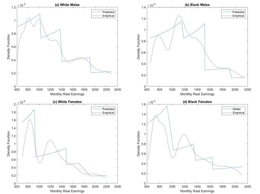
As a measure of model fit, Table 4 compares the sample statistics from
Table 1 with the predicted moments from the model using the estimated
33
The average productivity level is calculated by summing over the four firm types the
product of the productivity level, Pj , and the fraction of firms of that type, γj − γj−1 .
26Table 3: Firm Parameter Estimates for Male and Female Millennials
Males Females
Whites Blacks Whites Blacks
P1 1854.30 1759.10 1366.04 1383.22
(405.77) (304.67) (285.81) (142.59)
P2 2276.90 1993.10 2197.67 2066.91
(395.63) (307.77) (416.02) (295.56)
P3 3444.30 3353.20 2834.20 2608.56
(798.38) (647.84) (706.81) (381.45)
P4 5122.30 5027.80 4933.94 3410.85
(1932.38) (1669.24) (1618.60) (780.07)
γ1 0.4211 0.4839 0.3614 0.4059
(0.1703) (0.2070) (0.1551) (0.1151)
γ2 0.6974 0.8387 0.7952 0.7030
(0.1300) (0.1836) (0.1935) (0.1535)
γ3 0.9211 0.9677 0.9036 0.8515
(0.0756) (0.0629) (0.0787) (0.1000)
γ4 1.0000 1.0000 1.0000 1.0000
r 606.65 657.07 696.13 624.29
(17.96) (25.80) (9.19) (13.15)
wH1 1028.40 1148.70 909.40 918.25
(169.46) (200.30) (102.98) (90.52)
wH2 1375.70 1520.60 1479.69 1337.47
(180.16) (211.96) (253.66) (219.23)
wH3 1925.90 1942.10 1699.88 1640.79
(187.64) (182.69) (211.48) (224.41)
wH4 2292.11 2153.73 2211.17 2120.07
(34.10) (99.21) (69.61) (54.32)
Notes: Bootstrap standard errors are reported in paren-
theses.
parameters. As noted earlier, the predicted mean durations for both un-
employment and job spells are higher than the means observed in the
data, because the predicted means take into account the censoring rates
in the data. The predicted accepted earnings averages match quite well
for all four groups, as do the predicted transition rates to another job.
27The longer predicted mean unemployment duration for black males stems
from their lower arrival rate of job offers compared to white males, while
white and black females have higher arrival rates yielding shorter mean
unemployment durations. The shorter mean job duration for black males
compared to the other three groups results from their higher arrival rate
of job offers while employed as well as their slightly higher job destruction
rate. While a higher job destruction rate slows the rate at which black
males are moving up the wage ladder, a higher job-to-job transition rate
quickens it. On net, as demonstrated by a higher κ1 , black males are more
efficient than white males in moving up the wage ladder. However, black
females are the most efficient of the four groups given their relatively high
job arrival rate and lower job destruction rate.
In terms of the job-to-job transition rate, the fit is very good for all
four groups except black females. A closer look at this case reveals that
the estimation prefers a lower δ to fit the job duration data rather than
a higher δ to fit the transition data.34 The mean earnings are also quite
close with the model predicting lower mean earnings in all four cases and
the estimation results preserving the racial and gender gaps found in the
data. Finally, in terms of the correlations, the model predicts no correla-
tion between the unemployment spells and accepted earnings on the first
job, which matches the black males and black females well. It predicts
a positive correlation between job spells and accepted earnings as those
with higher earnings are be more likely to reject outside offers and stay
on their current job. This matches the correlations in the data for all four
34
The likelihood function for black females appears to be quite flat in the region
identifying δ. The estimates of λ0 and λ1 are fairly robust while the likelihood function
changes only a small amount with changes in δ that provide a better fit to the job-to-
job transitions but a worse fit to the job durations. Since the estimation method uses
a search algorithm to search over the wage cut estimates, there is no guarantee that it
returns the maximized log likelihood value. However, to determine whether this is a
problem we ran the estimation starting at several different values for δ. For all starting
values, the estimates we present were determined by the estimation routine to be the
estimates with the highest log likelihood value.
28You can also read